River Courses Affected by Landslides and Implications for Hazard Assessment: A High Resolution Remote Sensing Case Study in NE Iraq–W Iran


Abstract
: The objective of this study is to understand the effect of landslides on the drainage network within the area of interest. We thus test the potential of rivers to record the intensity of landslides that affected their courses. The study area is located within the Zagros orogenic belt along the border between Iraq and Iran. We identified 280 landslides through nine QuickBird scenes using visual photo-interpretation. The total landslide area of 40.05 km2 and their distribution follows a NW–SE trend due to the tectonic control of main thrust faults. We observe a strong control of the landslides on the river course. We quantify the relationship between riverbed displacement and mass wasting occurrences using landslide sizes versus river offset and hypsometric integrals. Many valleys and river channels are curved around the toe of landslides, thus producing an offset of the stream which increases with the landslide area. The river offsets were quantified using two geomorphic indices: the river with respect to the basin midline (Fb); and the offset from the main river direction (Fd). Hypsometry and stream offset seem to be correlated. In addition; the analysis of selected river courses may give some information on the sizes of the past landslide events and therefore contribute to the hazard assessment.1. Introduction
A landslide is a gravity-driven movement of rock, debris, or soils [1]. It results from the fluvial and glacial erosion of steep hillslopes in mountain belts [2–4]. Landslides are a major natural hazard because they are widespread, causing around 1,000 casualties per year and inflicting significant damages to infrastructures [5]. Landslides also modify natural environments, such as valley systems. The best example is landslide dams, including the 2010 Attabad Lake in northern Pakistan [6], the 2008 Tangjiashan Lake in China [7], and the 2,200-year-old Waikaremoana Lake in New Zealand [8–10], which usually occur when a landslide blocks the flow of a stream, causing a lake to form behind the dam [11]. The 300-meter-high Usoi landslide dam located in the Pamir Mountains (SE Tajikistan) is the highest dam, natural or man-made, in the world [12]. It was triggered by an earthquake on February 1911, and blocked the flow of the Murgab River [12–15].
An additional landslide effect on the drainage system is the offset of the main river, which forms when river channels curve around the toe of the landslide. Thus, as the rivers record past events, it might be possible to infer past landslide intensities from the river disturbances they inflicted. The analysis of selected river courses may give some information as to the sizes of past landslide events and therefore contribute to the hazard assessment. A river offset may form after landslide damming, when the stream has cut a new channel at the toe of the landslide. Most often, the newly created channel is shifted from the main direction of the stream. For instance, the Eureka River (western Canada) cut a new channel around the toe of a 20-meter-high landslide dam formed in 1990, abandoning the pre-landslide channel [16–18]. Incision has been rapid (almost 1 m/year) as the landslide was mainly constituted by wet earth and loose rocks. Some authors considered that the bends and morphology of the present day Eureka were caused by the bank incision and collapse during the flood events [19]. Similar examples can be found all over the planet. Mikoš et al. (2006) noticed that landslide-triggered debris flow filled the ravine of the Brusnik Stream in Slovenia. The channel was shifted to the left-hand side of the landslide, where the river incised its way [20]. Othus (2008) studied the landslides in the northern part of the Owyhee River, in southeastern Oregon (USA). He observed that river channels curved around the toe of landslides, creating offsets in the flows of the river channels [21].
Meandering is one of the most common morphologies of river channels [22]. Two types of river meandering are documented. The first type is the meandering caused by different circulation regimes. It occurs when a secondary circulation slowly brings water toward the inner bank and primary fast moving surface water flows toward the outer bank. Thus, channel curvature tends to be self-amplifying. As the bend grows, deposition on the inner bank often maintains a rough balance with erosion of the outer bank, keeping the width constant [23]. The second type of meandering occurs when rivers flow around the landslides toes [21], and/or tectonic features (faults or folds).
In this work, we examined river channels’ responses to landslides in an area located in the Zagros mountain belt. The objective of this study is to understand the effect of landslides on the drainage network, and quantify the relationship between the landslide area and river offsets. In addition, we demonstrate that river offsets could be a good indicator for landslide detection and could help the interpreter to detect past landslides during visual interpretation.
This study involved four main steps: (1) We prepared a landslide inventory map based on photo-interpretation; (2) We extracted the rivers and drainage basins. River offsets were calculated with respect to the theoretical basin midline and main river direction; (3) We created a hypsometric integral (HI) for the studied area; and (4) We performed statistical comparisons between river offsets, landslide areas and hypsometric values. This paper is organized as follows: we introduce the study area (Section 2) before presenting and discussing the methodology of work and the available data (Section 3). In the last two sections, we discuss the relationship between landslides, HI values, and river displacements for both types of offsets, i.e., the river offsets obtained from the main river direction (Fd) and from the basin midline (Fb) calculations.
2. Study Area
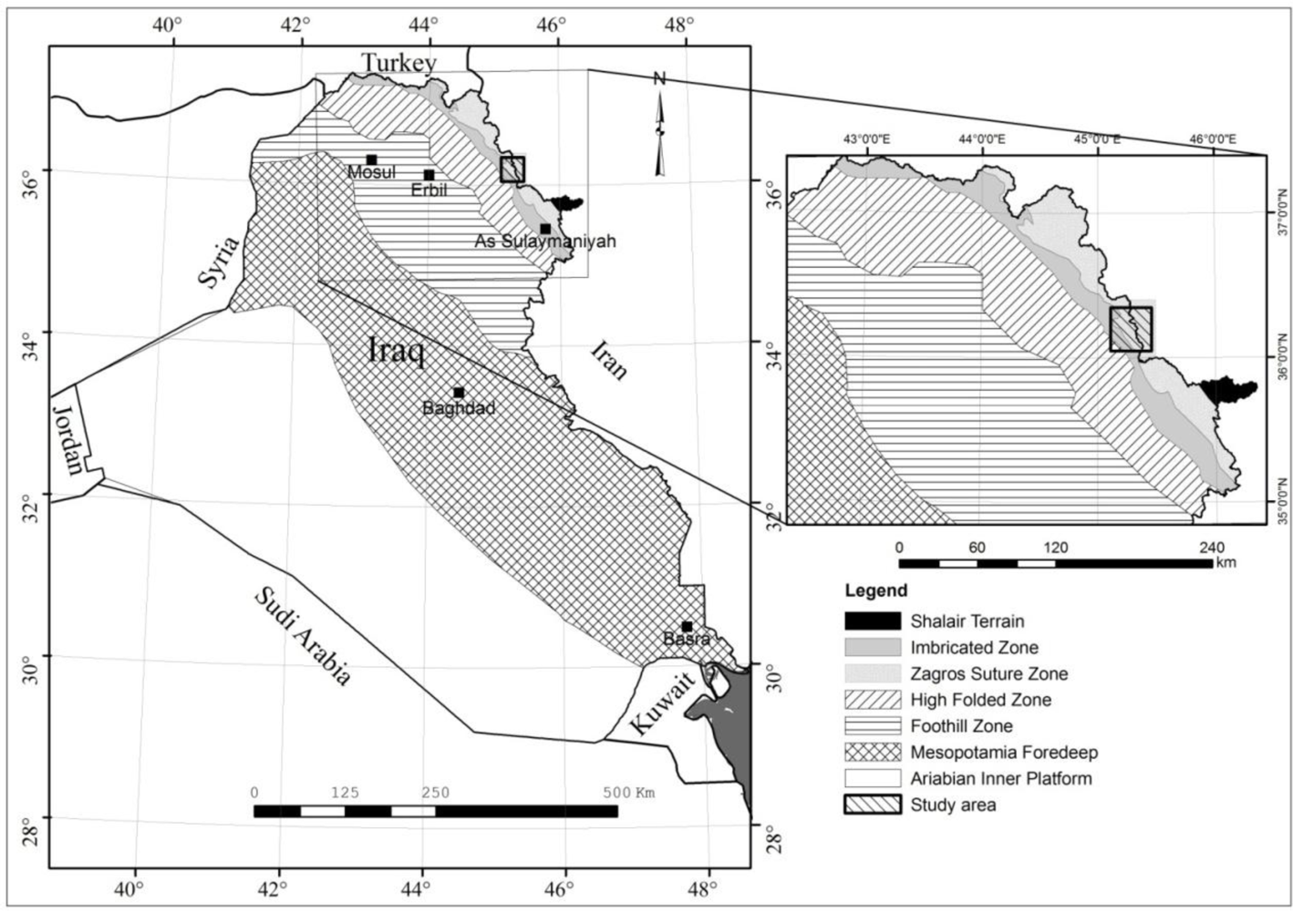
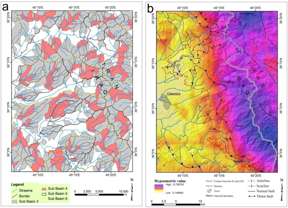
The study area is located between 36°00′–35°30′N latitudes; 45°00′–45°30′E longitudes, in the Zagros mountains, where mass movements threaten many towns and villages. It covers an area around 1047.7 km2 and encompasses the Sulaimaniyah Governorate (Kurdistan Region) in Iraq and the West Azerbaijan Province in Iran (Figure 1).
2.1. Geological Setting
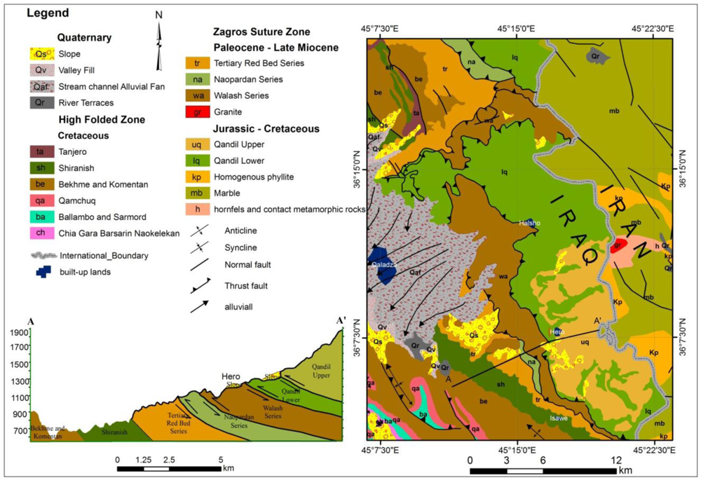
The NW-trending Zagros orogenic belt is a part of the Alpine–Himalayan mountain chain [24,25]. It is approximately 2,000 km long and extends from southeastern Turkey through Iraq to southern Iran. The study area lies within the Arabian Unstable Shelf, represented by the High Folded Zone (HFZ), the Imbricated Zone (IZ), and the Zagros Suture Zone (ZSZ) (Figure 1) [26]. The ZSZ was formed within the Neo Tethys as a result of the collision between the Arabian and the Iranian plates during the Late Cretaceous and Mio-Pliocene periods. Three NW-trending tectonic zones were formed in the ZSZ: the Qulqula-Khwarkurk Zone, which consists of radiolarian chert, mudstone, and limestone, conglomerates and basic volcanic rocks; the Penjween-Walash Zone, which consists of metamorphosed rocks, carbonate beds with volcanic and pyroclastic rocks; and, the Shalair Zone, which consists of meta-pelitic and meta-carbonates, volcanic, and metamorphosed rocks, in addition to different types of Quaternary sediments (river terraces, stream channel alluvial fans, slope sediments, valley fills). The Penjween-Walash Zone outcrops are only present in the eastern part of the study area. The Penjween-Walash Zone consists of nine structural units, four of them located in the Iranian part, and five in Iraq. Whereas the Penjween-Walash Zone located in Iran is comprised mainly of metamorphic rocks and granite [27], mainly sedimentary rocks, metamorphosed limestones with some serpentinite intrusions and a volcanic sequence including lava flows, ashes and dykes are found in the Iraqi region. The HFZ and the IZ are located in the western part of the study area; they include six sedimentary units (mainly limestones, marls, shales, dolomites, sandstones, mudstones, claystones and conglomerates) [26,28]. The HFZ and the IZ ages range from Middle Jurassic (Callovian) to Upper Cretaceous (Maastrichtian) (Figure 2) [26].
The IZ (a 25-km-wide narrow belt) and the HFZ have a similar structure [26]. The HFZ includes four small NW–SE oriented and asymmetrical anticlines and one syncline.
The study area is characterized by rugged topography in most parts; the eastern part of the study area is mainly of mountainous type. The western part of the study area comprises almost flat terrain, and hilly and undulated plains. The elevations range from 507 m to 2,415 m (a.s.l.). The slope gradient is from flat to 70°. This landscape results from the combined effects of tectonic uplift, erosion, and differences in rock strengths.
2.2. Climate
The study area is characterized by large seasonal variations in precipitation, temperature and evaporation, represented by dry summers and wet winters (Figure 3). Most of the entire annual precipitation (859.1 mm) occurs from October to May. January shows the highest precipitation with an average value of 198.2 mm. Monthly temperatures vary between −0.6 °C (January) and 37.3 °C (August). The snowfalls occur within 10.65 days per year in average between November and April. Above 1,500 m, heavy snowfall occurs in the winter (Figure 3). Heavy rainfall, heavy snowfall and rapid snow melting subsequent to sudden change in temperature, lead to the incidence of landslides in spring.
2.3. Landslides
The study area is affected by frequent landslide occurrences for natural environmental and human-induced reasons. Natural factors include a very rugged topography inducing strong variations in altitude and slope and a relatively heterogeneous geology, in addition to the rapid snow melting in spring and seasonal precipitations, which create super-saturation with water that increases the internal water pore pressure. Human activities which can cause slope failures include civil engineering activities like road cuts, overloading of the top or undercutting of the toe of slopes, and unsuitable agricultural practices [29].
The most widely used classification scheme developed by Varnes (1978) divides landslides into different types according to the material and the type of movement [30,31]. This classification distinguishes five types of mass movement (falls, topples, slides, spreads, and flows) in addition to combinations of these principal types along with types of material (bedrock, coarse soils, and predominant fine soils).
3. Methodology
3.1. Material
We used two orthorectified ASTER DEMs (Digital Elevation Models). These DEMs were extracted from ASTER Nadir (N) and backward looking (3B) bands (0.76–0.86 μm), The ASTER level 1A system scenes were acquired on 7 August 2006 and 24 August 2003 with a resolution of 15 m. In addition, we used nine QuickBird scenes obtained from the Ministry of Planning (Iraq) and acquired on 29 August 2006. These scenes are orthorectified, and radiometrically corrected eight-bit scenes, with 0.6 m spatial resolution. QuickBird scenes have three visible spectral bands, blue (0.45 to 0.52 μm), green (0.52 to 0.60 μm) and red (0.63 to 0.69 μm) [32].
Moreover, we digitalized nine geological maps, including 44 major landslides, from previous reports of Bolton (1954), Paver and Scholtzh (1955), Buday and Suk (1978) and Abdulaziz, et al. (1983) [33–36].
Environment for Visualizing Images (ENVI) software was used to perform the data operations (layer stack, mosaic, subset and stretch). River network, watershed boundaries, and hypsometry were extracted using TecDEM 2.2, a MATLAB-based software, which permits the extraction of geomorphologic indices from digital elevation models [37,38]. Additional GIS operations (Base map preparation, extraction of basins midlines, line to points conversion and calculation of areas) were made using ArcGIS10 with river bathymetry toolkit (RBT) and Hawth’s analysis tools. Statistical analyses were performed using R-based scripts.
3.2. Methods
3.2.1. Landslide Delineation
Remote sensing data can be used to detect a landslide over a large area. High-resolution satellite data are thus a useful tool for studying landslides [5]. The availability of new satellite data with better spatial and spectral resolution permitted the use of satellite data instead of aerial photographs for a better detection and investigation of landslides. It allows a quick detection and mapping of landslides. We prepared an inventory map of landslides from two sources. First, existing geological maps [33–36] with mapped landslides were scanned and georeferenced. We completed this data, with the interpretation and digitization of QuickBird scenes using ArcGIS10 software. The landslide boundaries were identified from the satellite data based on characteristics such as tone, texture, the headwall scarps, and associations like the pathway of the material movement, and fragments of transferred materials. We used Varnes’ (1978) classification to classify the landslides. We partly verified our observations by field survey in different parts of the study area.
3.2.2. Geomorphic Indices
Drainage network analysis is a powerful tool to investigate major landslides. The use of geomorphic indices derived from DEM allows the characterization and comparison of landscapes. After mosaic and subset ASTER DEM, the HI values, the DFb, the DFd, watersheds and drainage networks were extracted from the 15-m ASTER DEM data and analyzed using TecDEM 2.2.
We selected 122 landslides that lie within distance of 50 m near the valleys using valley shapefiles and the digitized landslide polygons. From these 122 landslides, we selected 61 landslides located near bended rivers. We could not involve the rest of 59 landslides, which are within the distance of 50 m near the valleys. Some of them are within big landslides and are already included and the other landslides are very small within major streams, and do not cannot affect major rivers. We converted the river line segments, near the landslides to points, where the interval between points was <20 m, and then calculated the point’s coordinates. We subsequently delineated the main rivers’ directions, which were calculated from the regressions of the points upstream and downstream from the bended rivers.
Midline Determination, Main River Direction and River-Offset Calculation
Two river offsets’ distances were calculated. We then tested the two different methods, the basin midline and main valley direction for their sensitivity to detect changes perpendicular to the main channel direction. The first one is the DFb. It is calculated by measuring the maximum perpendicular distance from river to the basin midline (Figure 4(a)), and the second is the DFd. It is calculated by measuring the maximum perpendicular distance from the river to the main river direction (Figure 4(b)). The river offset from the midline basin helps us to assess the affecting landslides for the bended basins when we cannot calculate the river offset from main river direction there. Drainage basins are symmetrical when external forces do not affect on them. Main rivers flow in the central part of the watershed and are almost superposed to the basin midline, the line located at the equal distance from both drainage divides. Landslides cause an offset of the river with respect to the basin midline. Therefore, an accurate midline extraction is important to determine the amount of offset and to detect the landslides and their influence in the stream basin. The river offset helps us to assess the effects of landslides by quantifying the variations of drainage symmetry along the stream length. We delineated the midline for basins where the main river was offset by a landslide. The midlines of basins were determined by using river bathymetry toolkit (RBT). This tool uses the Thiessen Polygons method and requires two shapefiles: the polygon layer of the basins, and the main valley lines of these basins. Both shapefiles should have a metric projection.
The main river direction is a fictitious line representing the straight line, which integrates the main line direction upstream and downstream from the river offset (Figure 4(b)). Figure 4(b) shows sub-basin no. 25, where two major landslides (extent up 2.07 and 1.8 km2) have bent the river with a maximum distance of 244 m and 503 m with respect to the basin midline. Hawth’s analysis tools in ArcGIS 10 were used to convert the stream polyline to points and calculate the point’s coordinates; we then extracted the points upstream and downstream from the offset to calculate the main river direction. The line best fitting these points represents the main river direction.
The Hypsometric Integral Map (HI)
The hypsometric integral (HI) is a suitable parameter to distinguish between different evolutionary stages in landscape development [39,40]. We used the HI to identify the stage of landscape development and quantify the relationship between the HI and distance of river offset. Hypsometry represents the amount of surface located above a given elevation. If the HI below 0.35 characterizes a monadnock phase for the HI in the range 0.35–0.6, the area is in the equilibrium (mature) phase; if the HI is above 0.6, the area is in a youthful stage in its landscape development [40]. As the HI value is sensitive to the erosion [40], we used a moving window with 400 pixels, which represents ∼6 km to create the HI map using the TecDEM software. The HI is generally derived for a particular area or a drainage basin and does not depend on scale. It is thus possible to compare large and small surfaces. According to Pike and Wilson (1971) the HI equation [41] is
3.2.3. Statistics
After preparing the HI map and calculating the landslides area and river-offset distance, we examined the relations between landslide area, river offset, and hypsometry through linear regressions. Linear regressions were made using scripts based on R language. The first regression was preformed with the natural logarithm of the DFd, the second was carried out with the natural logarithm of the DFb, and the third with the natural logarithm of geometric mean of the DFd and river width (ln (Gm)). The purpose of using the Gm is to illustrate the width of river influence on the river offset. In addition, we analyze a linear regression between the landslide areas (A) and the DFb. The basic relationship of river-offset distance and area of landslide can be expressed as follows:
We tested the relation of the mean of the HI values (Hmean) with the mean of the DFb, and with the DFd. The basic relationship of river-offset distance and area of landslide can be expressed as follows:
4. Results
4.1. Landslide Inventory Map
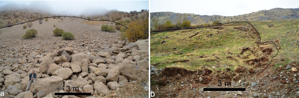
Several types of landslides are common in the study area: rock falls, toppling, which covered 0.77% of the total landslides in the study area (Table 1), and occurred in different lithological units along steep slopes and gorges. Occurrences are independent or collective. Landslides caused road blockings and many nearby towns suffer from incidents from time to time. A large mass of rock fall was witnessed recently in this area that blocked the main roads. Big blocks of heavily fractured limestone fall from a steep slope cliff due to gravity. The volumes of these blocks of limestone reach to bigger than 1,300 m3. Rockslide is common in hard rock and occurs along a shear surface, which is planar [1]. This type of slide, in addition to earth slide, covered ∼43.35% of the total landslides of the study area (Table 1). It damages more than rock fall and is thus more dangerous. Slumps or spoon-like landslides covered 46.77% of the total landslides of the study area (Table 1), occurring in different lithological units along steep slopes, gorges, and shear surfaces (Figure 5(b)). Slump landslides are common in weak layers (rock slump and earth slump), especially when they have been softened by percolation of rainwater [1]. Figure 6 shows that slump sliding threatens the roads in different sites of the study area. The old and active slump landslides, particularly the large ones, might suffer in the future from small landslides. Among the numerous landslides observed in the region, the best examples are those that occurred around the towns of Hero and Halsho (Figure 5(a)). This area is affected by extensive blocks (some as big as 1 km2) and slump sliding, which mainly occur on the slopes of deeply eroded valleys and in areas where clay layers underlie hard rock accumulations. In addition, clastic debris and rock flow is common in the weak layers and soil. It covers 9.112% of the total landslides of the study area (Table 1). Especially in the north–northwest of the study area, the clastics of debris are usually fine-grain-sized. The sliding has a hazardous effect on engineering structures. Some of the landslides are from as far back as the early Pleistocene period [34].
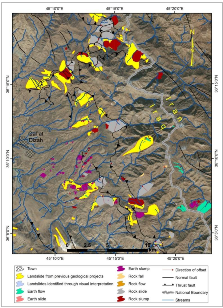
Figure 7 shows the inventory of landslides in our study area. 44 major landslides were digitized from nine previous geological maps. We identified 280 additional landslides from QuickBird images.
The landslides cover a total area of 40.05 km2 and the total study area is 1,047.7 km2. The density is 0.27 landslides/km2 Landslides’ rate of total area is 3.8 %. The densest distribution of landslides occurs along a NW–SE trend due to the influence of structures related to the Zagros orogenic belt (Figure 7). The smallest landslide is 60 m2. On the other hand, the 10 largest landslides have an area >1 km2 of them are located in the ZSZ (northeast–eastern part of the study area), covering a total area of 15.4 km2 within the Naopurdan-Walash Group (Paleocene–Oligocene). The Naopurdan-Walash group consists of gray shales with thin beds of green greywacke, and lenticular volcanic rocks.
In the study area, 22 major landslides offset the rivers in 20 basins, whereas, 61 landslides (the above 22 mentioned in addition to 39 other landslides) contributed to the bending of the river channels around the toes of the landslides. Most of them are the result of slump sliding and rockslides.
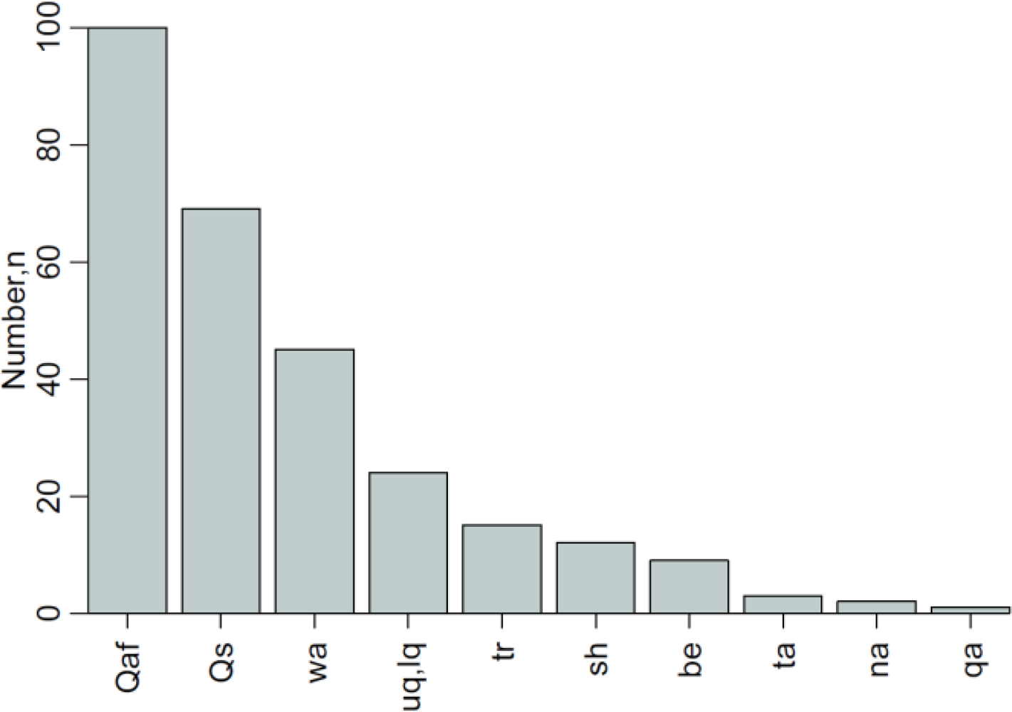
Figure 8 shows the formations most commonly involved in landslides throughout the study region. Rock types have been broadly classified into “coherent,” “moderate,” and “weak” units based on the dominant character of each as inferred from unit descriptions and from qualitative assessments made in the field. For example, rocks of the Walash series (e.g., wa, Table 2) were considered coherent, while Tanjero Formation (e.g., ta, Table 2) were classified as weak. Figure 8 illustrates that both coherent and weak rocks occur with high frequency in the landslides mapped.
4.2. Geomorphic Indices
We extracted the drainage network of Lesser Zab River Basin and 4, 46, 201 and 882 sub-basins corresponding to the sixth, fifth, fourth and third Strahler order rivers. Respectively, from ASTER DEM using TecDEM (Figure 9(a)). We selected 20 sub-basins, affected by the 22 major landslides: (1, 7 and 12 sub-basins from the fifth, fourth and third Strahler orders respectively.
Figure 9(b) displays the hypsometry for the study area. The HI values range from 0.74 to 0.14; the values (>0.35) were found to the east of the contact between the ZSZ and the IZ. The topography is thus mainly controlled by the active thrust faults. The HI values above 0.6, which indicate very young topography, are located in three patches: two of them are located on the international boundary towards the south of the study area, while the third is located in the northern Iranian part of the study area.
We calculate DFd for all landslides, in addition to the river width. The major landslides cover about 2.6 km2, caused a maximum offset of 572 m for Alawa River (50 m width) near Halshow Town. Figure 10 and 11 show examples of landslides, which bent the rivers. Figures 10(a) and 11(a–c) represent rock slump landslides, while Figure 10(b) represents earth flow landslide. Figure 11(a) show one of the three major landslides near Hero Town, which caused the offset Darwena River of 430 m.
Figure 12 represents the rose diagram for the angle between the major landslide and the major thrust fault. The major landslides, which caused the river offsets, mostly have orthogonal direction to the strike of the thrust fault or have a big angle with them (Figure 7 and 12).
4.3. Statistics of River Offsets
Since the stream offsets and landslide sizes in the study area cover several orders of magnitude, we use log–log representations of 59 bent rivers and we left three of them to test the equation. We find a good linear relation between the log of DFd and the log of the landslides areas (Figure 13(a)). The minimum value of DFd was 4.1, and the maximum was 572. Figure 13(b) shows a direct relation between the log of the (Gm) and log of the landslide area. For both plots (Figure 13(a,b)) the statistical correlations are > 0.97, and the exponents were 1.77 and 1.96, respectively.
We find a good linear relation between the DFb and the landslide areas, where the statistical correlation was >0.96 (slope = 4,039) (Figure 14(a)). Figure 14(b) shows a direct relation between the log of Gm the DFb and the log of the landslide areas, where the statistical correlation was ∼0.9 (the exponent = 1.55).
The plot in Figure 15(a) illustrates a direct linear relationship between the DFb and the mean of HI values in the bent valley, where the statistical correlation was >0.78 (the slope is 0.00065 and the intercept is 0.22). The plot in Figure 15(b) shows a direct linear relationship between the DFd and the HI values, where the statistical correlation was >0.7, (the slope is 0.00025 and the intercept is 0.27).
5. Discussion
The understanding of past failures is essential in the assessment of landslide hazard [45]. The removing of old landslides from the Earth’s surface due to natural erosion processes gives a misperception for landslide hazard assessment in the past. Therefore, the analysis of a selected river’s courses, in addition to the landslides inventory, may give more information to evaluate the hazard assessment of the past.
We prepared the landslide inventory map through photo-interpretation QuickBird satellite images for the entire study area. The dominant direction for the migration of river caused by landslides is NW–NE direction. The results suggest that the main thrust fault controls the distribution and the sliding direction of landslides. We found that the distance from the thrust fault is inversely proportional to the concentration of landslides. Most of the large landslides are in contact with the main thrust faults or located at a distance of <3,600 m from 92% of total landslides.
The river-offset distance increases with the HI mean value of the bent river (Figure 15(a,b)) because the triggered area has a lower topography than the crown of the landslide, but is still higher than the river. On the other hand, the HI value is dependent on curvature of the surface. Therefore, the major landslides have a direct linear relationship with the cliff elevation; the curvature of the major landslides is less concave than the small landslides near the rivers.
The HI of the longitudinal profile of the stream ranges 0.21–0.46 represents the concave shape. The HI of the longitudinal profile of the stream value, which is <0.21, represents the flat area, and the HI of the longitudinal profile of the stream value, which is >0.46, represents the convex shape. In Figure 15(b), we excluded the small landslides from the regression because of their minor effect on rivers, which is smaller than the topography effects that influence the HI value. For HI values are affected by topography of neighboring major river basins, landslides >0.46 and <0.21 are not used in the regression with DFd since river offsets near the major upstream and the major downstream are incorporated within those values.
This study indicates that the direct relationship between the river-offset distance and the landslide area can be formed in quantitative relationships (Figures 13(a) and 14(a,b)). We test two river offset measures: the first was DFd and the second was the DFb. The exponent for the DFd (α) is 1.77, and the exponent for the DFb is 1.56. We tested three bent rivers with the DFd equation (Equation (2)) to find the potential area of the landslides which caused them (Table 3). The calculated areas from the equation show error with the real areas (0.6–3.5%). The errors may be from the angle between the landslides and the origin river direction. We could use Equation (2) to estimate the size of old landslides and quantify the relationship of the landslide area to the distance of the river offset. This equation is useful for estimating local landslide potential and thus hazard assessment.
The symmetry factor (T) is a good index for demonstrating the stream deviations, as the stream suffers from lateral migration due to the influence of tectonic [37,42–44]. The main difference between river offset triggered by a landslide and a tilted basin is that the river offset induced by landslide is local, while in the tectonically tilted basin, the entire basin midline is shifted, regardless of the direction of the river offset. This may be the reason for the difference between the exponents of the DFd and the DFb in Figure 13(a,b). The DFd is more realistic than the DFb.
6. Conclusions
We mapped 280 landslides in an area located along the Iraq–Iran border through the analysis of nine QuickBird scenes. The most representative landslides include rock falls, debris flows, translational slides, and slumps. The densest distribution of landslides in the study area has a NW–SE trend due to the tectonic influence of the Zagros orogenic belt. We also analyzed river offsets and hypsometry in the areas affected by landslides. This study also indicates that landslides cause many rivers offsets and that there is a correlation between the offset amount and the landslide area. A correlation between the offset amount and the hypsometry was also found. The major landslides, which caused the offset for the rivers have orthogonal direction to the strike of the thrust fault or have a big angle with it. This demonstrates that the main thrust fault controls the sliding direction of landslides. The HI values range from 0.74 to 0.14; the threshold number of 0.35 is occurs at the contact between the ZSZ and the IZ and it nearly corresponds to the main thrust fault. The hypsometry suggests a strong control of main thrust on the topography.
The statistical analysis of landslides allows assessing the size of the expected river offsets. Further studies could be performed to find out if the valley size prevents river offset development and which size is required instead to make a landslide generate a lake.
Acknowledgments
The research was supported by the Ministry of Higher Education and Scientific Research of Iraq (MoHESR), and by Deutscher Akademischer Austauschdienst (DAAD). We are grateful to the Geological Survey of Iraq and Ministry of Planning in Iraq for supporting the data and fieldwork.
References
- Blasio, F.V.D. Introduction to the Physics of Landslides; Springer: New York, NY, USA, 2011. [Google Scholar]
- Luckman, P.G.; Gibson, R.D.; Derose, R.C. Landslide erosion risk to New Zealand pastoral steeplands productivity. Land Degradation and Development 1999, 10, 49–65. [Google Scholar]
- Ouimet, W.B. Landslides associated with the May 12, 2008 Wenchuan earthquake: Implications for the erosion and tectonic evolution of the Longmen Shan. Tectonophysics 2010, 491, 244–252. [Google Scholar]
- Larsen, I.J.; Montgomery, D.R.; Korup, O. Landslide erosion controlled by hillslope material. Nature Geosci 2010, 3, 247–251. [Google Scholar]
- Lillesand, T.M.; Kiefer, R.W.; Chipman, J.W. Remote Sensing and Image Interpretation, 5th ed; John Wiley & Sons, Inc: Hoboken, NJ, USA, 2004. [Google Scholar]
- Petley, D.N.; Rosser, N.J.; Karim, D.; Wali, S.; Ali, N.; Nasab, N.; Shaban, K. Non-Seismic Landslide Hazards along the Himalayan Arc. In Geologically Active; Willians, A.L., Pinches, G.M., Chin, C.Y., McMorran, T.J., Massey, C.I., Eds.; CRC Press: London, UK, 2010; pp. 143–154. [Google Scholar]
- Cui, P.; Dang, C.; Zhuang, J.-Q.; You, Y.; Chen, X.-Q.; Scott, K.M. Landslide-dammed lake at Tangjiashan, Sichuan province, China (triggered by the Wenchuan Earthquake, May 12, 2008): Risk assessment, mitigation strategy, and lessons learned. Environ. Earth Sci 2012, 65, 1055–1065. [Google Scholar]
- Howard-Williams, C.; Law, K.; Vincent, C.L.; Davies, J.; Vincent, W.F. Limnology of Lake Waikaremoana with special reference to littoral and pelagic primary producers. New Zealand Journal of Marine and Freshwater Research 1986, 20, 583–597. [Google Scholar]
- Newnham, R.M.; Lowe, D.J.; Matthews, B.W. A late-Holocene and prehistoric record of environmental change from Lake Waikaremoana, New Zealand. The Holocene 1988, 8, 443–454. [Google Scholar]
- Allan, J.C.; Stephenson, W.J.; Kirk, R.M.; Taylor, A. Lacustrine shore platforms at Lake Waikaremoana, North Island, New Zealand. Earth Surface Process. Landf 2002, 27, 207–220. [Google Scholar]
- Highland, L.M.; Bobrowsky, P. The Landslide Handbook—A Guide to Understanding Landslides; US Geological Survey: Reston, VA, USA, 2008; p. 1325. [Google Scholar]
- Schuster, R.L.; Alford, D. Usoi Landslide Dam and Lake Sarez, Pamir Mountains, Tajikistan. Environ. Eng. Geosci. 2004, X, 151–168. [Google Scholar]
- Alford, D.; Schuster, R.L. Usoi Landslide Dam and Lake Sarez, An Assessment of Hazard and Risk in the Pamir Mountain, Tajikistan; UN: New York, NY, USA and Geneva, Switerland, 2000. [Google Scholar]
- Risley, J.C.; Walder, J.S.; Denlinger, R.P. Usoi Dam wave overtopping and flood routing in the Bartang and Panj Rivers, Tajikistan. Natural Hazards 2006, 38, 375–390. [Google Scholar]
- Risley, J.; Walder, J.; Denlinger, R. Usoi Dam Wave Overtopping and Flood Routing in the Bartang and Panj Rivers, Tajikistan; US Geological Survey: Reston, VA, USA, 2006; p. 29. [Google Scholar]
- Evans, S.G.; Mugnozza, G.S.; Strom, A.; Hermanns, R.L. Landslides from Massive Rock Slope Failure; Springer: Dordrecht, The Netherlands, 2006; p. 49. [Google Scholar]
- James, L.A. Tailings fans and valley-spur cutoffs created by hydraulic mining. Earth Surface Process. Landf 2004, 29, 869–882. [Google Scholar]
- Miller, B.G.N.; Cruden, D.M. The Eureka River landslide and dam, Peace River Lowlands, Alberta. Can. Geotech. J 2002, 39, 863–878. [Google Scholar]
- Morgan, A.J.; Paulen, R.C.; Slattery, S.R.; Froese, C.R. Geological Setting for Large Landslides at the Town of Peace River, Alberta; Open File Report 2012-04; Alberta Geological Survey: Edmonton, AB, Canada, 2012. [Google Scholar]
- Mikoš, M.; Brilly, M.; Fazarinc, R.; Ribičič, M. Strug landslide in W Slovenia: A complex multi-process phenomenon. Eng. Geol 2006, 83, 22–35. [Google Scholar]
- Othus, S.M. Comparison of Landslides and Their Related Outburst Flood Deposits, Owyhee River, Southeastern Oregon, M.Sc. Thesis; Central Washington University, Ellensburg, WA, USA. 2008.
- Imran, J.; Parker, G.; Pirmez, C. A nonlinear model of flow in meandering submarine and subaerial channels. Fluid Mech 1999, 400, 295–331. [Google Scholar]
- Goudie, A.S. Encyclopedia of Geomorphology; Routledge Ltd: New York, NY, USA, 2006; p. 1156. [Google Scholar]
- Alavi, M. Tectonics of Zagros Oroginic Belt of Iran: New data and interpretations. Tectonophysics 1994, 229, 221–238. [Google Scholar]
- Alavi, M. Regional stratigraphy of the Zagros Fold—Thrust Belt of Iran and its proforeland evolution. Am. J. Sci 2004, 304, 1–20. [Google Scholar]
- Jassim, S.Z.; Goff, J.C. Geology of Iraq; Dolin: Brno, Czech Republic, 2006. [Google Scholar]
- Nezhad, J.E. The Geological Map of Mahabad Quadrangles, Sheet NI-38-15 (map no. B4), Scale 1:250000; Geological Survey of Iran: Tehran, Iran, 1973. [Google Scholar]
- Sisakian, V.K. The Geology of Erbil and Mahabad Quadrangle Sheet NJ-38-14 and NJ-38-15 (GM 5 and 6), Scale 1:250 000; Iraq Geological Survey: Baghdad, Iraq, 1998. [Google Scholar]
- Sissakian, V.K.; Ahad, I.D.A.; Qambar, A.S. Series of Geological Hazards Map of Iraq Sulimanyah Quadrangle, Sheet No. NI-38-3, Scale 1:250 000; Iraq Geological Survey: Baghdad, Iraq, 2004. [Google Scholar]
- Varnes, D.J. Slope Movement Types and Processes. In Special Report 176: Landslides: Analysis and Control; Schuster, R.L., Krizek, R.J., Eds.; Transportation and Road Research Board, National Academy of Science: Washington, DC, USA, 1978; pp. 11–33. [Google Scholar]
- Dikau, R.; Brunsden, D.; Schrott, L.; Ibsen, M.L. Landslide Recognition: Identification, Movement and Causes; Wiley: Chichester, UK, 1996. [Google Scholar]
- DigitalGlobe, Quickbird Imagery Products: Product Guide; Version 4.7.1; DigitalGlobe, Inc.: Longmont, CO, USA, 2006.
- Abdulaziz, M.T.; Ibraheem, F.A.; Sebesta, J.; Hassan, A. The Lesser Zab River Basin Project, Photo-Engineering Geological and Geomorphological Mapping; Iraq Geological Survey: Baghdad, Iraq, 1983; p. 87. [Google Scholar]
- Buday, T.; Suk, M. Report on the Geological Survey in NE Iraq between Halabjaand Qala′adiza; Iraq Geological Survey: Baghdad, Iraq, 1978. [Google Scholar]
- Paver, G.L.; Consultant, M.B.; Scholtzh, H.C. Six Monthly Report July to December 1955; Iraq Geological Survey: Baghdad, Iraq, 1955; Volume 5. [Google Scholar]
- Bolton, C.M. Geological Map Kurdistan Series, Sheet K4, Scale 1/100000, Rania; Iraq Geological Survey: Baghdad, Iraq, 1954. [Google Scholar]
- Shahzad, F.; Gloaguen, R. Tecdem: A matlab based toolbox for tectonic geomorphology, Part 2: Surface dynamics and basin analysis. Comput. Geosci 2011, 37, 261–271. [Google Scholar]
- Shahzad, F.; Gloaguen, R. Tecdem. A matlab based toolbox for tectonic geomorphology, Part 1: Drainage network preprocessing and streamprofile analysis. Comput. Geosci 2011, 37, 250–260. [Google Scholar]
- Pērez-Peňa, J.V.; Azaňōn, J.M.; A.Azor, Calhypso. An arcgis extension to calculate hypsometric curves and their statistical moments. Applications to drainage basin analysis in SE Spain. Comput. Geosci 2009, 35, 1214–1223. [Google Scholar]
- Strahler, A.N. Hypsometric (area–altitude) analysis of erosional topography. Geol. Soc. Am. Bull 1952, 63, 1117–1142. [Google Scholar]
- Pike, R.J.; Wilson, S.E. Elevation-relief ratio, hypsometric integral and geomorphic area-altitude analysis. Geol. Soc. Am. Bull 1971, 82, 1079–1084. [Google Scholar]
- Garrote, J.; Cox, R.T.; Swann, C.; Ellis, M. Tectonic geomorphology of the southeastern mississippi embayment in northern mississippi, USA. Geol. Soc. Am. Bull 2006, 118, 1160–1170. [Google Scholar]
- Garrote, J.; Heydt, G.G.; Cox, R.T. Multi-stream order analyses in basin asymmetry: A tool to discriminate the influence of neotectonics in fluvial landscape development (madrid basin, central spain). Geomorphology 2008, 102, 130–144. [Google Scholar]
- Mahmood, S.A.; Gloaguen, R. Appraisal of active tectonics in hindu kush: Insights from dem derived geomorphic indices and drainage analysis. Geosci. Front 2012, 3, 1–22. [Google Scholar]
- Guzzetti, F.; Carrara, A.; Cardinali, M.; Reichenbach, P. Landslide hazard evaluation: A review of current techniques and their application in a multi-scale study, central italy. Geomorphology 1999, 31, 181–216. [Google Scholar]


| Landslides Type | No. of Landslides | Min. Area (m2) | Max. Area (km2) | Total Landslides Area (m2) | Landslides Rate of Total Area % |
|---|---|---|---|---|---|
| Earth slump | 113 | 70.36 | 695,342.82 | 4,492,088.79 | 11.22 |
| Earth flow | 48 | 108.55 | 1,946,147.7 | 3,634,582.13 | 9.072 |
| Earth slide | 8 | 5,486.62 | 108,680.25 | 198,098.5 | 0.494 |
| Rock fall | 33 | 59.97 | 8,4172.38 | 308,628.57 | 0.77 |
| Rock flow | 2 | 3,394.91 | 64,757 | 16691.81 | 0.04 |
| Rock slide | 37 | 202.67 | 2,654,951.78 | 17,161,058.98 | 42.85 |
| Rock slump | 39 | 208.78 | 1,429,172.22 | 14,241,804.52 | 35.554 |
| All types | 280 | 59.97 | 2,654,951.78 | 40,052,953.3 | 100% |
| Code | Formation | Description and Rock Type | Relative Strength |
|---|---|---|---|
| Qaf | Alluvial Fan | Sand, gravel, and silt-forming floodplains and filling channels of present streams. | Weak |
| Qs | Slope | sandy and silty clayey materials | Weak |
| Wa | Walash Series | Basic volcanic sequence includes agglomerate, lava flows, pillow lavas and ashes with associated dykes. The volcanic are associated with a thick sedimentary sequence, thick limestones, red mudstones and clastics. | Coherent |
| uq,lq | U. and L. Qandil | Sheared limestones, phyllitas and massive metamorphosed limestone, with some serpentinite intrusions. | Coherent |
| Tr | Red Bed | Conglomerates, red shales, red sandstones, red mudstones. | Coherent |
| sh | Shiranish | Thinly well-bedded marly and chalky limestones, followed (upwards) by thin bedded or papery marl, blue and gray in color with some marly limestone beds | Moderate |
| be | Bekhme, Komentan | Well-bedded limestones, dolomostones, marly limestone and rare marl | Coherent |
| ta | Tanjero | Shale, claystone, sandstone and siltstone some conglomerates | Weak |
| na | Naopardan Series | Shales, limestone, tuffaceous slates, felsitic volcanics, basic conglomerate, greywackes and sandy shale. | Coherent |
| qa | Qamchuq | Massive limestones and dolomites, usually dark gray in color. | Coherent |
| DFd (m) | Measured Area (m2) | Area from Equation | Error (m2) | Error % |
|---|---|---|---|---|
| 12.7 | 3,592.14 | 3,614.24 | 22.1 | 0.62 |
| 27.8 | 14,573.83 | 14,453.28 | 120.5 | 0.83 |
| 50 | 39,456.67 | 40,875.28 | 1418.6 | 3.6 |
Share and Cite
Othman, A.A.; Gloaguen, R. River Courses Affected by Landslides and Implications for Hazard Assessment: A High Resolution Remote Sensing Case Study in NE Iraq–W Iran. Remote Sens. 2013, 5, 1024-1044. https://doi.org/10.3390/rs5031024
Othman AA, Gloaguen R. River Courses Affected by Landslides and Implications for Hazard Assessment: A High Resolution Remote Sensing Case Study in NE Iraq–W Iran. Remote Sensing. 2013; 5(3):1024-1044. https://doi.org/10.3390/rs5031024
Chicago/Turabian StyleOthman, Arsalan A., and Richard Gloaguen. 2013. "River Courses Affected by Landslides and Implications for Hazard Assessment: A High Resolution Remote Sensing Case Study in NE Iraq–W Iran" Remote Sensing 5, no. 3: 1024-1044. https://doi.org/10.3390/rs5031024