Indoor Localization Algorithms for an Ambulatory Human Operated 3D Mobile Mapping System

Abstract
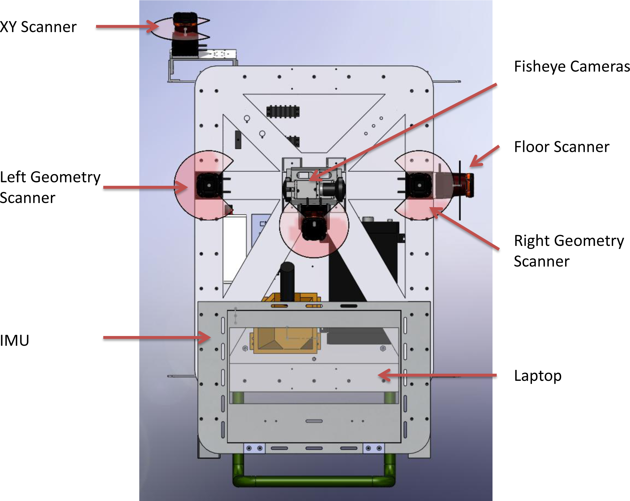
:1. Introduction
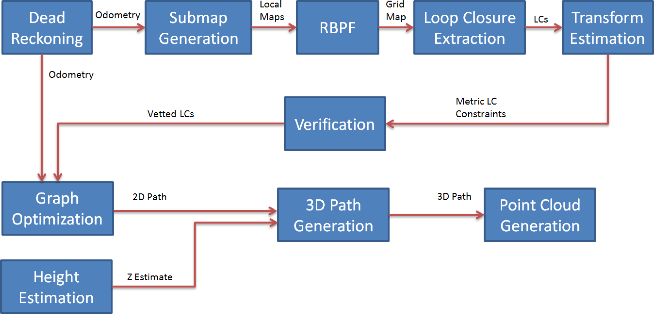
2. Localization Algorithms
2.1. 2D Dead Reckoning
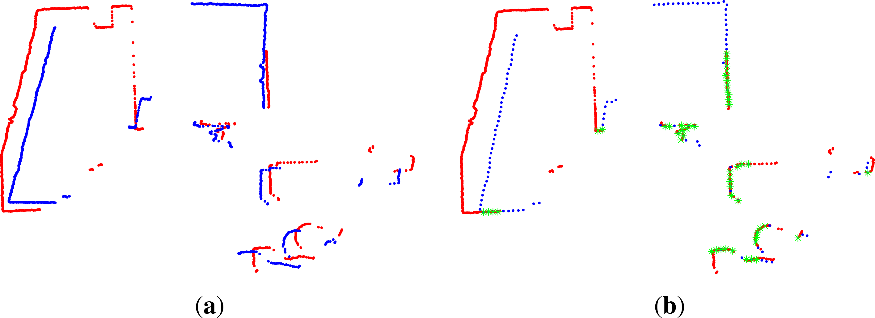
- Given an initial transform T (·, μ0), points in Q are matched to their nearest neighbors in set P.
- Assuming a fixed T (·, μ0), an optimal set of inlier points Df is identified.
- Using inlier set Df, the transform parameters μ are recovered using a first-order Taylor expansion and solving for the optimal linear estimate of μ [24].
2.2. Submap Generation
2.3. Rao-Blackwellized Particle Filtering
2.4. Loop Closure Extraction
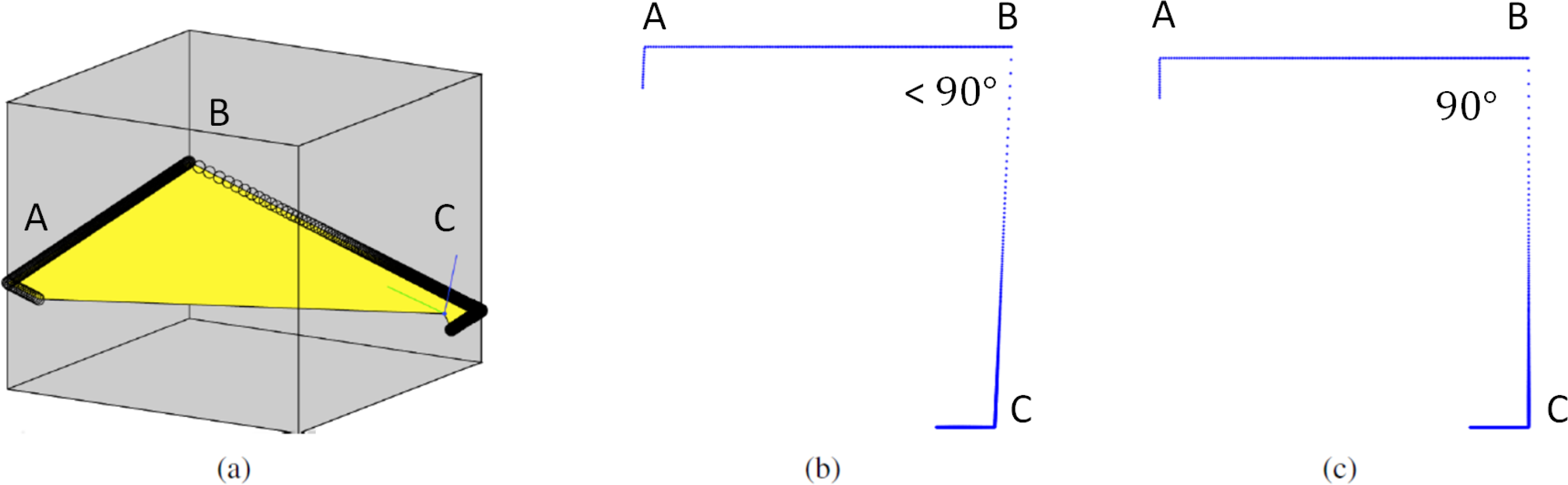
2.5. Loop Closure Transform Estimation

| 1: μ0 ← initial estimate 2: S0 ← random_chromosomes(μ0) 3: while Sn+1 ≠ Sndo 4: Rn ← ∅︀ 5: for si ∈ Sn do 6: ri ← ICP (si) 7: Rn ← Rn ∪ {ri} 8: end for 9: Rn ← best_subset_of (Rn) 10: Sn+1 ← Rn ∪ make_children(Rn) 11: end while 12: return μ and Df from best chromosome. |
2.6. Loop Closure Transformation Verification
2.7. Height Estimation
2.8. 3D Path Generation
2.9. Point Cloud Generation
3. Results
3.1. FGSM Performance Evaluation
3.2. Effect of Discretization on the FGSM Algorithm
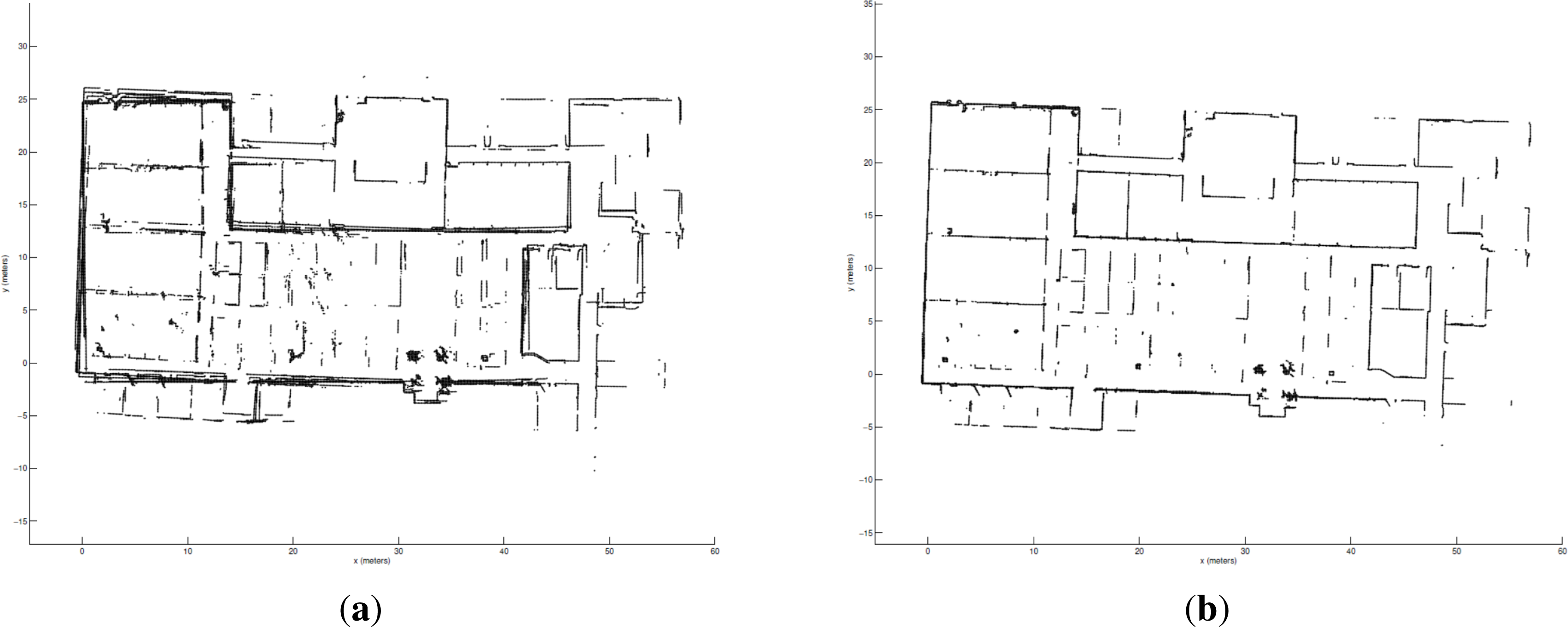
3.3. End-To-End System Results
4. Applications
5. Conclusions and Future Work
Acknowledgments
Conflict of Interest
References
- Li, R. Mobile mapping: An emerging technology for spatial data acquisition. Photogramm. Eng. Remote Sens 1997, 63, 1085–1092. [Google Scholar]
- Karimi, H.; Khattak, A.; Hummer, J. Evaluation of mobile mapping systems for roadway data collection. J. Comput. Civil Eng 2000, 14, 168–173. [Google Scholar]
- Ellum, C.; El-Sheimy, N. Land-based mobile mapping systems. Photogramm. Eng. Remote Sens 2002, 68, 13–28. [Google Scholar]
- Holenstein, C.; Zlot, R.; Bosse, M. Watertight Surface Reconstruction of Caves from 3D Laser Data. Proceedings of the IEEE International Conference on Intelligent Robots and Systems, San Francisco, CA, USA, 25–30 September 2011; pp. 3830–3837.
- Bosse, M.; Zlot, R. Continuous 3D Scan-Matching with a Spinning 2D Laser. Proceedings of the IEEE International Conference on Robotics and Automation, Kobe, Japan, 12–17 May 2009; pp. 4312–4319.
- Hesch, J.; Mirzaei, F.; Mariottini, G.; Roumeliotis, S. A Laser-Aided Inertial Navigation System (L-INS) for Human Localization in Unknown Indoor Environments. Proceedings of the IEEE International Conference on Robotics and Automation, Anchorage, AK, USA, 3–7 May 2010; pp. 5376–5382.
- Bosse, M.; Zlot, R.; Flick, P. Zebedee: Design of a spring-mounter 3-D range sensor with application to mobile mapping. IEEE Trans. Robot 2012, 28, 1104–1119. [Google Scholar]
- Moghadam, P.; Bosse, M.; Zlot, R. Line-Based Extrinsic Calibration of Range and Image Sensors. Proceedings of the IEEE International Conference on Robotics and Automation, Karlsruhe, Germany, 6–10 May 2013.
- Fallon, M.; Johannsson, H.; Brookshire, J.; Teller, S.; Leonard, J. Sensor Fusion for Flexible Human-Portable Building-Scale Mapping. Proceedings of the IEEE/RSJ International Conference on Intelligent Robots and Systems, Vilamoura, Portugal, 7–12 October 2012; pp. 4405–4411.
- Foxlin, E. Pedestrian tracking with shoe-mounted inertial sensors. IEEE Comput. Graph. Appl. 2005, 25, 38–46. [Google Scholar]
- Angermann, M.; Robertson, P. Footslam: Pedestrian simultaneous localization and mapping without exteroceptive sensors—Hitchhiking on human perception and cognition. Proc. IEEE 2012, 100, 1840–1848. [Google Scholar]
- Moafipoor, S.; Grejner-Brzezinska, D.; Toth, C. Multisensor Personal Navigator Supported by Adaptive Knowledge Based System: Performance Assessment. Proceedings of the IEEE/ION Position, Location, and Navigation Symposium, Monterey, CA, USA, 5–8 May 2008.
- Bok, Y.; Jeong, Y.; Choi, D. Capturing village-level heritages with a hand-held camera-laser fusion sensor. Int. J. Comput. Vis 2011, 94, 36–52. [Google Scholar]
- Google Trekker. Available online: http://www.google.com/maps/about/partners/streetview/trekker/ (accessed on 20 November 2013).
- Shen, S.; Michael, N.; Kumar, V. Autonomous Multi-Floor Indoor Navigation with a Computationally Constrained MAV. Proceedings of the IEEE International Conference on Robotics and Automation, Shanghai, China, 9–13 May 2011; pp. 20–25.
- Bachrach, A.; Prentice, S.; He, R.; Henry, P.; Huang, A.; Krainin, M.; Maturana, D.; Fox, D.; Roy, N. Estimation, planning, and mapping for autonomous flight using an RGB-D camera in GPS-denied environments. Int. J. Robot. Res 2012, 31, 1320–1343. [Google Scholar] [Green Version]
- Shen, S.; Michael, N.; Kumar, V. Autonomous Indoor 3D Exploration with a Micro-Aerial Vehicle. Proceedings of the IEEE International Conference on Robotics and Automation, Saint Paul, MN, USA, 14–18 May 2012; pp. 9–15.
- Chen, G.; Kua, J.; Naikal, N.; Carlberg, M.; Zakhor, A. Indoor Localization Algorithms for a Human-Operated Backpack System. Proceedings of the 3D Data Processing, Visualization, and Transmission, Paris, France, 17–20 May 2010.
- Liu, T.; Carlberg, M.; Chen, G.; Chen, J.; Kua, J.; Zakhor, A. Indoor Localization and Visualization Using a Human-Operated Backpack System. Proceedings of the International Conference on Indoor Positioning and Indoor Navigation, Zurich, Switzerland, 15–17 September 2010.
- Kua, J.; Corso, N.; Zakhor, A. Automatic loop closure detection using multiple cameras for 3D indoor localization. IS&T/SPIE Electron. Imag. 2012. [Google Scholar] [CrossRef]
- Newman, P.; Cummins, M. FAB-MAP: Probabilistic localization and mapping in the space of appearance. Int. J. Robot. Res 2008, 27, 647–665. [Google Scholar]
- Bosse, M.; Zlot, R. Keypoint design and evaluation for place recognition in 2D lidar maps. Robot. Auton. Syst 2009, 57, 1211–1224. [Google Scholar]
- Granstrom, K.; Callmer, J.; Nieto, J.; Ramos, F. Learning to Detect Loop Closure from Range Data. Proceedings of the IEEE International Conference on Robotics and Automation, Kobe, Japan, 12–17 May 2009; pp. 15–22.
- Bosse, M.; Zlot, R. Map matching and data association for large-scale two-dimensional laser scan-based SLAM. Int. J. Robot. Res 2008, 26, 667–691. [Google Scholar]
- Lenac, K.; Mumolo, E.; Nolich, M. Robust and Accurate Genetic Scan Matching Algorithm for Robotic Navigation. Proceedings of the International Conference on Intelligent Robotics and Applications, Aachen, Germany, 6–8 December 2011; pp. 584–593.
- Phillips, J.; Liu, R.; Tomasi, C. Outlier Robust ICP for Minimizing Fractional RMSD. Proceedings of the 3-D Digital Imaging and Modeling, Montreal, QC, Canada, 21–23 August 2007; pp. 427–434.
- Grisetti, G.; Stachniss, C.; Burgard, W. Non-linear constraint network optimization for efficient map learning. IEEE Trans. Intell. Transp. Syst 2009, 10, 428–439. [Google Scholar]
- Dellaert, F.; Kaess, M. Square root SAM: Simultaneous localization and mapping via square root information smoothing. Int. J. Robot. Res 2006, 25, 1181–1203. [Google Scholar]
- Fitzgibbon, A. Robust Registration of 2D and 3D Point Sets. Proceedings of the British Machine Vision Conference, Manchester, UK, 10–13 September 2001; pp. 662–670.
- Censi, A. An ICP Variant Using a Point-to-Line Metric. Proceedings of the IEEE International Conference on Robotics and Automation, Pasadena, CA, USA, 19–23 May 2008; pp. 19–25.
- Chetzerikov, D.; Svirko, D.; Stepanov, D.; Kresk, P. The Trimmed Iterative Closest Point Algorithm. Proceedings of the International Conference on Pattern Recognition, Quebec, Canada, 11–15 August 2002.
- Besl, P.; McKay, N. A method for registration of 3D shapes. IEEE Trans. Pattern Anal. Mach. Intell 1992, 14, 239–256. [Google Scholar]
- Thrun, S.; Burgard, W.; Fox, D. Probabilistic Robotics; The MIT Press: Cambridge, MA, USA, 2005. [Google Scholar]
- Murphy, K. Bayesian Map Learning in Dynamic Environments. Proceedings of the Neural Information Processing Systems (NIPS), Denver, CO, USA, 30 November 1999.
- Grisetti, G.; Stachniss, C.; Burgard, W. Improving Grid-based SLAM with Rao-Blackwellized Particle Filters By Adaptive Proposals and Selective Resampling. Proceedings of the IEEE International Conference on Robotics and Automation, Barcelona, Spain, 18–22 April 2005; pp. 2432–2437.
- Jain, A.; Murty, M.; Flynn, P. Data clustering: A review. ACM Comput. Surv 1999, 31, 264–323. [Google Scholar]
- Man, K.; Tang, K.; Kwong, S. Genetic Algorithms, Concepts and Designs; Springer: London, UK, 1999. [Google Scholar]
- Martinez, J.; Gonzalez, J.; Morales, J.; Mandow, A.; Garcia-Cerezo, J. Mobile robot motion estimation by 2D scan matching with genetic and itertive closest point algorithms. J. Field Robot 2006, 23, 21–34. [Google Scholar]
- Barla, A.; Odone, F.; Verri, A. Histogram Intersection Kernel for Image Classification. Proceedings of the International Conference on Image Processing Barcelona, Spain, 14–17 September 2003; 3, pp. 513–516.
- Pomerleau, F.; Colas, F.; Siegwart, R.; Magnenat, S. Comparing ICP variants on real-world data sets. Auton. Robot 2013, 34, 133–148. [Google Scholar]
- Wold, S.; Esbensen, K.; Geladi, P. Principal component analysis. Chemom. Intell. Lab. Syst. 1987, 1, 37–52. [Google Scholar]
- Turner, E.; Zakhor, A. Seattle, WA, USA, 29 June–1 July 2013.
- Cheng, P.; Anderson, M.; He, S.; Zakhor, A. Texture Mapping 3D Planar Models of Indoor Environments with Noisy Camera Poses. To Appear In Proceedings of the SPIE Electronic Imaging Conference, San Francisco, CA, USA, 2–6 February 2014.
- Trimble TIMMS. Available online: http://www.trimble.com/Indoor-Mobile-Mapping-Solution/ (accessed on 20 November 2013).


| σT (m) | Libpointmatcher [40] | Hybrid-GSM [25] | FGSM (proposed) |
|---|---|---|---|
| 0.25 | 93% | 90% | 94% |
| 0.5 | 89% | 91% | 95% |
| 1.0 | 82% | 89% | 94% |
| 2.0 | 68% | 73% | 91% |
| 3.0 | 58% | 59% | 85% |
| 5.0 | 45% | 42% | 75% |
| 8.0 | 30% | 36% | 66% |
| 10.0 | 25% | 30% | 62% |
| σθ (degrees) | Libpointmatcher [40] | Hybrid-GSM [25] | FGSM (proposed) |
|---|---|---|---|
| 18 | 74% | 60% | 92% |
| 30 | 59% | 44% | 84% |
| 45 | 45% | 31% | 73% |
| 60 | 34% | 24% | 63% |
| 90 | 25% | 17% | 49% |
| 180 | 17% | 11% | 37% |
| (σT, σθ) (meters, degrees) | Libpointmatcher [40] | Hybrid-GSM [25] | FGSM (proposed) |
|---|---|---|---|
| (0.25, 18) | 74% | 60% | 91% |
| (0.5, 30) | 55% | 43% | 84% |
| (1.0, 45) | 42% | 33% | 74% |
| (2.0, 60) | 28% | 21% | 61% |
| (3.0, 90) | 18% | 11% | 45% |
| (5.0, 180) | 9% | 6% | 33% |
| Subtask | Running Time (min) |
|---|---|
| Dead Reckoning | 3 |
| Submap Generation | 50 |
| RBPF Grid Mapping | 60 |
| Loop Closure Detection | 10 |
| Transform Estimation | 2 |
| Verification | 1 |
| Graph Optimization | 2 |
| Height Estimation | 10 |
| 3D Path Generation | 1 |
© 2013 by the authors; licensee MDPI, Basel, Switzerland This article is an open access article distributed under the terms and conditions of the Creative Commons Attribution license ( http://creativecommons.org/licenses/by/3.0/).
Share and Cite
Corso, N.; Zakhor, A. Indoor Localization Algorithms for an Ambulatory Human Operated 3D Mobile Mapping System. Remote Sens. 2013, 5, 6611-6646. https://doi.org/10.3390/rs5126611
Corso N, Zakhor A. Indoor Localization Algorithms for an Ambulatory Human Operated 3D Mobile Mapping System. Remote Sensing. 2013; 5(12):6611-6646. https://doi.org/10.3390/rs5126611
Chicago/Turabian StyleCorso, Nicholas, and Avideh Zakhor. 2013. "Indoor Localization Algorithms for an Ambulatory Human Operated 3D Mobile Mapping System" Remote Sensing 5, no. 12: 6611-6646. https://doi.org/10.3390/rs5126611