An Operational System for Estimating Road Traffic Information from Aerial Images

Abstract

Given that ground stationary infrastructures for traffic monitoring are barely able to handle everyday traffic volumes, there is a risk that they could fail altogether in situations arising from mass events or disasters. In this work, we present an alternative approach for traffic monitoring during disaster and mass events, which is based on an airborne optical sensor system. With this system, optical image sequences are automatically examined on board an aircraft to estimate road traffic information, such as vehicle positions, velocities and driving directions. The traffic information, estimated in real time on board, is immediately downlinked to a ground station. The airborne sensor system consists of a three-head camera system, a real-time-capable GPS/INS unit, five industrial PCs and a downlink unit. The processing chain for automatic extraction of traffic information contains modules for the synchronization of image and navigation data streams, orthorectification and vehicle detection and tracking modules. The vehicle detector is based on a combination of AdaBoost and support vector machine classifiers. Vehicle tracking relies on shape-based matching operators. The processing chain is evaluated on a large number of image sequences recorded during several campaigns, and the data quality is compared to that obtained from induction loops. In summary, we can conclude that the achieved overall quality of the traffic data extracted by the airborne system is in the range of 68% and 81%. Thus, it is comparable to data obtained from stationary ground sensor networks.

1. Introduction

1.1. Motivation

The ongoing growth of our metropolises and regional conurbations makes it necessary to have adequate methods for road traffic monitoring and traffic guidance. Everyday operations for generating road traffic information mainly rely on stationary ground infrastructure, such as induction loops, radar sensors and traffic cameras. All of the information is usually collected, processed and interpreted in traffic control centers. There, measures are adopted for the optimization of traffic flow. These are then transferred to the roads via intelligent traffic guidance systems. With a sparse distribution or even lack of traffic sensors on side roads, these traffic monitoring systems are generally blind to the situations on minor roads. Using floating car data (FCD, e.g., [1,2,3]) or floating phone data (e.g., [4]), it is possible to get information of the traffic situation for some minor roads without stationary ground sensors [5]. It was shown that these systems are well suited for the estimation of travel times, even without the use of stationary traffic sensors. However, these data are incomplete in terms of wide area coverage and are not sensitive to short-term congestion. In the case of disasters, with the damage of ground infrastructure or extensive power blackouts, such systems would fail. This would result in a complete lack of information and not just with respect to side roads.

Several projects that contribute to area-wide traffic monitoring by remote sensing based on airborne optical and SAR sensors are currently running at the German Aerospace Center (DLR) or have already been concluded (e.g., [6,7,8,9]). Meanwhile, an airborne optical system for traffic monitoring with real-time capability has been developed [10]. This system allows automatic traffic data extraction from image sequences in real time on board the aircraft. Data are immediately sent to the ground via air-ground microwave radio relay or laser link [11]. The system is also able to send current orthorectified and georeferenced images to the ground that can be used to produce situation maps, which are required by relief forces [12]. The benefits of an airborne remote sensing system for the generation of traffic information are its universal and selective applicability, since it is not limited to major roads, and that it is independent of ground infrastructure. Even the ground station is designed to be self-sustaining, supplied by a power generator. Combined with the disaster management tool (DMT, e.g., [13]), it is possible to provide traffic information and aerial images to the relief forces in affected areas in real time, even in the event of a complete breakdown of ground infrastructure. Furthermore, the generated traffic information can be used for short-term prognoses of the traffic situation [14].

In contrast to our previous publication [10,15], where the used hardware architecture and components are described in detail (Section 2), this paper is focused on the automatic traffic data acquisition. In particular, the methods and algorithms for the generation of road traffic information (Section 3) are addressed, and the quality of the traffic data for the data set shown in Section 4 was evaluated (Section 5).

1.2. Related Work

There are many approaches for vehicle detection from aerial images. Extensive overviews are given in [16,17,18]. Generally, vehicle detection is performed using implicit or explicit models. The first approaches with explicit models used a simple rectangular mask for detection [19,20]. Later on, extensions to 3D wire fame models were introduced and combined with classification methods [21]. One of the most mature works using hierarchical vehicle models was shown in [22], which was used for road verification. Most approaches are not concerned with computation time, which is a critical condition for real-time applications, such as the system proposed in this work. Implicit models in combination with neural networks were used by [23,24] with promising results. In [25], an online boosting procedure for efficient training data collection was utilized. They used different features, which can all be calculated very quickly using integral images or integral histograms. Finally, a non-parametric algorithm performs clustering of the calculated confidence values. An interesting work was presented in [26]. They introduced new features for vehicle detection, i.e., color probability maps and pairs of pixels. These led to very large feature sets, and partial least squares were used for feature transformation. The authors of [27] use rotation invariant histograms of oriented gradients [28] and an adaptive boosting classifier. Even though the authors use the same kind of imagery as the presented work (see Section 2.1), the overall approach is not in the operational state. In the last few years, there have been many approaches to vehicle detection working with images from UAVs [29,30,31,32]. These systems have a small payload, which leads to limited coverage compared to airborne systems. Additionally, the regulatory framework to fly UAVs remains uncertain in some countries, while a concept for the country-wide operationalization of the presented system can be found in [33].

In recent decades, several methods for automatic tracking algorithms have been examined. The first results were achieved based on the optical flow [34,35] from the image sequences of stationary ground traffic cams. Further developments in vehicle tracking were carried out by [36], who used a deformable vehicle template model, and by [37], who presented a 3D modeling approach. Airborne frame cameras with a low or medium frame rate require alternative methods. Fundamental research on this topic based on change detection algorithms was done by [38,39]. While these algorithms work fine on moving objects, they are not suitable for recording vehicles that are static. In [6,7], detection-based tracking algorithms on a medium frame rate system were presented. There, tracking was performed by an intelligent attribution of vehicle detections in consecutive images. A similar approach was transferred to low frame rate sequences in [40]. Later on, the focus of development shifted to combined detection tracking approaches, in which the tracking was based on template matching (e.g., [8,41,42]). The tracking results shown in this paper are based on the latter approaches. At the current operational state, all vehicle are tracked individually. Newer approaches for aerial vehicle tracking use more advanced prediction methods, such as Kalman filtering and, furthermore, track multiple objects simultaneously [43]. In [44], particle filtering for multiple vehicles is presented, which is currently integrated with the operational system.

Due to the increased number of high resolution satellite imagery systems in the last decade, there have been many approaches for vehicle detection [45,46,47,48,49] and even tracking from single-pass images [50,51,52]. However, these systems are not comparable to the presented work. Satellites have revisit times of several days and are mostly solar synchronic. Thus, the possible applications seem to be quite restricted. Even so, these approaches are quite interesting; to our best knowledge, there is no operational system that uses traffic data from such systems.

As a matter of course, all optical imaging system strongly rely on weather and illumination conditions. During night time or bad weather conditions, active sensors, such as LiDAR [53,54,55] or SAR [56,57,58], may be applicable. Furthermore, infrared sensors are capable of detecting still and recently active vehicles [59]. Within the same project as the presented work, approaches for vehicle detection from airborne SAR systems are developed [60], which are based on the DLR’s in-house E-SAR system [61].

2. System Overview

The real-time system for traffic monitoring from aerial images can be divided into several sub-systems. The on-board system consists of a sensor system, a computer network system and a radio link. The ground system consists of a receiving antenna and a computer network. Figure 1 shows an overview of the system part on-board the aircraft. The on-board computer network system consists of industrial PCs with up-to-date hardware (Core-i-7 CPU, 16 GB RAM, SSD drives, NVIDIA GeForce 9800 GTX GPU/512 MB memory/compute capability 1.1) and a Gigabit switch. Image sequences are acquired by the 3K+ camera system. Flight position and attitude is recorded synchronously by an IGI GPS/Inertial Navigation System (INS) with real-time capabilities. Images are read out from the cameras and synchronized with the data stream recorded by the GPS/INS navigation unit. Further processing steps performed by the on-board computers are image storage and image/navigation data stream synchronization, direct georeferencing/orthorectification and the generation of road traffic information. After the traffic information is extracted, images are sent to the ground together with the extracted traffic data. In order to reduce the data traffic of the downlink, only every third image of the sequence is sent to the ground, which is sufficient for continuous mapping. Another function of the on-board computer network is to steer the beam antennas of the directional radio link system. It keeps the sending antennas aligned to the ground station regardless of the position and attitude of the aircraft. The radio link system operates in the C-band, works bidirectionally and delivers a data bandwidth of 7–12 Mbit/s for distances of up to 100 km. The ground antenna has a parabolic design with a diameter of 60 cm and is pivot mounted in azimuth and elevation. Aircraft and the ground station exchange GPS positions via the radio link for dynamic antenna alignment.

On the ground, traffic information, such as vehicle positions and velocities, is refined and aggregated on Navteq road sections. A road section is a polygon of several nodes that locates the primary middle axis positions of roads. It follows the road until an intersection is reached or an attribute of the road changes. In these cases, a new section begins. On two-way roads, the opposite driving direction is represented by separate polygons with a reverse course. A typical road level-of-service display of a traffic portal uses aggregated traffic information. Therefore, each vehicle is allocated to its corresponding road section, and the average values of velocity and vehicle density are calculated for each section. Aggregated traffic information is transferred to an internet traffic portal server. This allows security and emergency authorities and organizations to follow the current traffic situation (road level-of-service) and derive traffic prognoses based on this traffic data. The underlying road map of the traffic portal is also Navteq-based. Georeferenced images of the airborne system are mosaicked at the ground station and transferred to an Internet portal, as well.

Figure 1. Overview of the airborne component of the on-board sensor system.

Figure 1. Overview of the airborne component of the on-board sensor system.

Due to limited camera capacities for high frame rates, the sensor system records images in the so-called burst modes. Camera bursts are short sequences with a high image repetition rate. After an image burst, the cameras stop for several seconds until the next burst is triggered. Each burst consists of three consecutive exposures with a 1.25 to 2 Hz frame rate (configurable). An image burst is recorded every 7 s. Thus, the amount of image data is significantly reduced compared to a continuous exposure mode with a high frame rate. At a typical flight speed of 70 m/s, there is a 30% overlap between the first images of each burst at a flight height of 1500 m. Vehicle detection is performed on each first image of the burst, and vehicle tracking is done using consecutive image pairs within the burst (Section 3).

In another configuration, the radio downlink system is replaced by an optical laser transmission, called FELT (free-space experimental laser terminal; [11]). It consists of an airborne optical terminal that aligns the laser towards the ground station. The digital data stream is modulated to the laser light signal. On the ground, the transportable optical ground station receives the signal.

The aircraft system is usually controlled by two on-board operators. For future purposes, a fully automatic system will be designed to handle operations without any on-board interaction. In this case, interventions will be commanded from the ground via radio link. Based on the present system, we are currently developing a small lightweight version of an airborne traffic monitoring system that can be installed on helicopters or small aircraft [10].

2.1. DLR’s In-House “3K/3K+” Camera System

Since 2004, an optical airborne sensor system based on commercial off-the-shelf cameras had been developed at the DLR and employed for many campaigns. The 3K camera has a significantly higher frame rate than metric camera systems, which allows it to record movements on the ground, like road traffic. The 3K camera consists of three Canon 1Ds Mark II cameras with a 36 × 24 mm CMOS chip at 16.7 Megapixels. The maximum frame rate is 3 fps. The cameras are arranged to provide one nadir view and two oblique views. In 2011, the camera system was replaced by its successor, the 3K+ camera system. The platform design of the 3K was kept, but the cameras were replaced by Canon 1Ds Mark III cameras. These cameras provide a resolution of 21 Mpix each and a higher frame rate of up to 5 Hz. A detailed comparison between of the 3K and 3K+ system can be found in [10]. With the use of 50-mm objective lenses, the nadir ground sampling distances for the 3K/3K+ sensor at a typical flight height of 1000 m above ground are 15 cm versus 13 cm. With a (configurable) maximum tilt angle of ±32° of the side-looking cameras, both sensors have a footprint of 2560 m × 480 m at this flight height. The field of view (FOV) at the maximum angle is 104° across track and 26° in the flight direction. The maximum positioning error on the ground after georeferencing/orthorectification at a height of 1000 m is in the range of 1.4 m in the nadir to around 3 m at the edges of the FOV. The displacement between consecutive images of the same burst is less than 1 pixel, which is important for accurate velocity determination during tracking. Figure 2 shows the coverage in across and along track mode. The standard mode for traffic data acquisition is the across track burst mode (Figure 2, upper left illustration).

Figure 2. Ground coverage of the 3K/3K+ sensor system in continuous across track mode (lower left), across track burst mode (upper left) and continuous along track mode (right).

Figure 2. Ground coverage of the 3K/3K+ sensor system in continuous across track mode (lower left), across track burst mode (upper left) and continuous along track mode (right).

Exposures of the sensor are triggered by an external trigger box. The trigger box has an internal logic that produces pulses for the external trigger input of the cameras. It is activated manually by the camera operator on-board the aircraft when it reaches the flight strip. Exposure parameters and image recording can be triggered for the cameras with software via USB.

The airborne sensor system is usually operated on-board the DLR research aircraft, Dornier DO 228 and Cessna 208B Grand Caravan. These aircraft provide high performance concerning range (i.e., natical mile - NM) and endurance (DO 228: 1500 NM/9:00 h; Cessna: 1020 NM/6:30 h) and airspeed (i.e., knots true airspeed - KTAS) (DO 228: 220 KTAS; Cessna: 184 KTAS). The total cost of a flight hour is 1200 EUR for the Cessna and 1600 EUR for the DO 228. Compared to the total turnover and gains during major events, the costs for flight hours might be acceptable, not to mention flight costs versus information gain by additional products, such as maps during a disaster [12]. The lightweight version of the airborne system mentioned above already had its first flight with the DLR BO 105 helicopter in June 2014. Flight operation costs of the helicopter are comparable to that of the Cessna 208B.

2.2. Online Pre-Processing

In the first pre-processing step, the image stream of each camera and the data stream of the GPS/IMU navigation system are synchronized in each camera PC.

The next processing step is direct georeferencing/orthorectification. This is done only with the flight position, height and attitude data of the GPS/INS navigation unit without using any ground control points. The interior orientation of the cameras and the boresight misalignment between cameras and IMU has to be determined once prior to the real-time mission. Images are projected to a DEM using the algorithm presented in [62]. For real-time orthorectification, the code has been parallelized to run on NVIDIA graphics card GPUs in the CUDA programming environment. With this, the execution time of the orthorectification process for each image is reduced from 13 s, when executed on a CPU, to 250 ms on the GPU.

The projected images are passed to the traffic processor, which performs the traffic data extraction. After traffic processing, the traffic data and selected images are transferred to the sender PC (PC 5 in Figure 1) to transmit them directly to the ground station.

3. Methodology

In this section, the overall procedure for the generation of traffic information is presented. All processing steps for estimating road traffic information are performed on-board the aircraft. To fulfill the interface specification of the Internet traffic portal, only the conversion of the traffic information is done on the ground. In addition, another outlier correction procedure, which is done according to [41], can be activated at the ground station. This module was transferred to the ground in order to save computing power in the on-board system. After georeferencing of the images (Section 2.2), external geoinformation is used for delineation of road areas (Section 3.1). The following vehicle detection (Section 3.2) is performed in the regions of interest of the first image of each sequence (image burst). All detected vehicles are tracked by shape-based matching, as described in Section 3.3. The performance of the algorithms has to fulfill the time constraints given by the burst mode configuration, which limits the overall processing time to 7 s. Details of our strategy for saving computation time are given in the following section.

3.1. Image Preprocessing

Orthoimage preparation for vehicle detection is performed for each camera viewing direction. The images are overlayed with road axes obtained from a Navteq database. This is done in order to reduce the search area for vehicle detection and limit it to road areas. In this preprocessing step, it is possible to choose roads of certain level types by the number of lane categories or other road attributes. All of the pixels located between a certain width buffer along the road axes are selected as the region-of-interest. A typical value used for the road buffer width is 22 m, because it works for all types of road categories. It is sufficient to cover motorways with four or more lanes while taking into account the errors in the location of road axes and image georeferencing. If the extraction of traffic information is limited to minor roads (e.g., in city regions), the buffer width can be reduced. In a future version of the processing chain, we plan to adapt the road buffer width to the lane categories.

All regions-of-interest are aligned in the road direction by resampling, which leads to straightened and rotated road snippets. All vehicles appear horizontal. Thus, there is no need for rotational invariant feature calculation during detection, which may be computational expensive compared to the used Haar-like features. A look-up table for the transformation of pixel and UTM coordinates from the straightened road images back to the original images is created. It contains both the pixel coordinates in the straightened image and the UTM coordinates of each node of the respective Navteq section. Thus, each vehicle position detected in the straightened roads image can be transformed into the coordinate system of the original image. 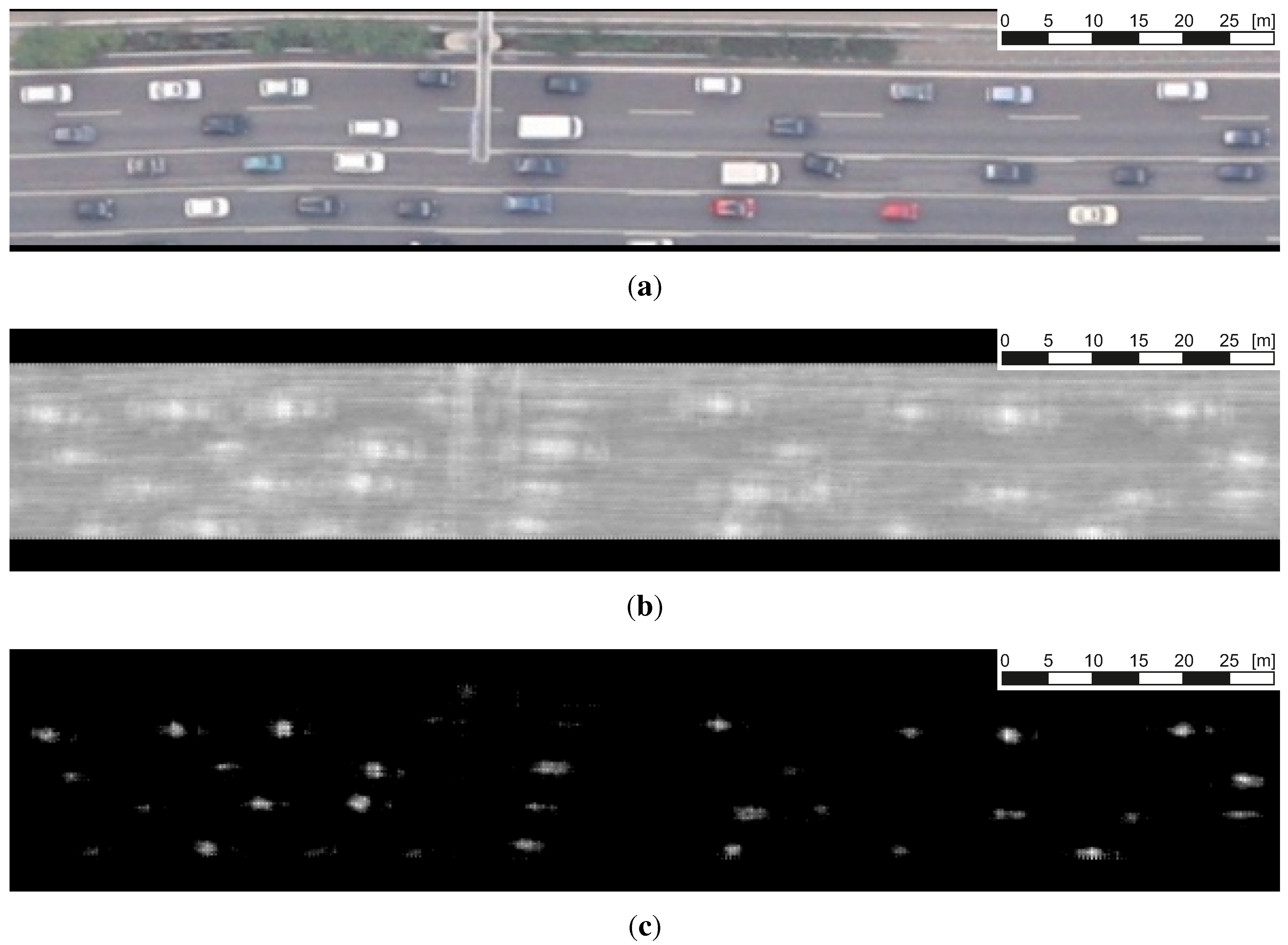Figure 3a shows the situation after road buffering and straightening. The images of the straightened roads obtained from each first image of an exposure burst are transferred to the next module of the traffic processor, the vehicle detector.

Figure 3. Results of the boosted classifier. (a) Straightened image; (b) boosting results; (c) boosting results after threshold.

Figure 3. Results of the boosted classifier. (a) Straightened image; (b) boosting results; (c) boosting results after threshold.

3.2. Vehicle Detection

We developed a processing procedure for fast vehicle detection, which consists of the following three stages:

• pre-classification with a boosted classifier;
• blob detection for reducing the number of vehicles hypothesis;
• final classification of the remaining hypothesis.

This stage-wise approach is able to fulfill the defined performance constraints.

Pre-Classification

During pre-classification, an extended set of Haar-like features [63] is used, which are based on features introduced in [64] and give a general description of different objects. Due to the large number of pixels covering one single vehicle in images with a ground sampling distance (GSD) of 20 cm, the overcomplete set of features contains nearly 2 million possible Haar-features for all image channels. Although the calculation of single features is very fast, as shown in [65], it is not feasible to calculate all features during classification, due to existing time constraints. Therefore, the pre-classification is performed by an adaptive boosting algorithm, also known as AdaBoost. Thus, necessary feature reduction is directly carried out during the training of the classifier. In general, AdaBoost builds a strong classifier F (x) as a linear combination of iteratively generated weak classifiers f^m (x):

$$F(x)\text{ = }{\sum }_{m=1}^M{f}^m(x)$$

(1)

Here, the sign of F (x) gives the predicted class label, while its absolute value is a confidence measure for this prediction. Different techniques, such as stumps or decision trees, can be used as weak classifiers. While decision trees are able to learn dependencies between features [66], we used stumps, because they can be evaluated faster, since only one binary threshold has to be evaluated. During the training, only the feature that produces the lowest weighted classification error is selected at each iteration. This leads to a drastic reduction of the overcomplete feature set. The training stops when the predefined threshold of test error is reached. The error rate was set to 2%, and the training finished after 70 iterations. Therefore, only 70 features have to be calculated during classification. Figure 3 shows an example of the classification result. In the first image (Figure 3a), an original straightened road is display. The next image (Figure 3b) shows the complete range of possible confidence values from −1 (black color) to 1 (white color), where high values stand for vehicles and lower values correspond to the background. After setting all negative confidence values to 0, vehicles already become clearly visible in Figure 3c.

In this work, the classification is performed by gentle AdaBoost [66], which is stated to have better performance [67] compared to the original discrete [68] and real AdaBoost [69], due to less severe weighting of wrongly labeled or unrepresentative training samples.

Blob Detection

Following the pre-classification, neighboring pixel with positive confidence values are grouped by finding zero crossings. As can be seen in Figure 4a, a huge number of image regions do not correspond to vehicles. To reduce the number of possible image regions for later final classification, we detect very fast keypoints, as described in [70]. To do this, the image is smoothed using a median filter, resulting in smoothed image Ĩ. Then, points Ĩ (m + dR_α) within a predefined radius R, i.e., approximately the size of vehicles, are evaluated according to the gray value difference τ to the center point Ĩ (m). Here, dR_α = (R cos (α) ; R sin (α)) and α is varying between 0 and π. If |Ĩ (m) − Ĩ (m + dR_α)| ≤ τ and if |Ĩ (m) − Ĩ (m − dR_α)| ≤ τ, then m is not a keypoint. Thus, blobs of specific characteristics can be found within the positive valued image regions. Optimal parameters for R, τ and the number of points on the radius, i.e., the number of varying α, were found by 5-fold cross-validation. The red circles in Figure 4b mark the remaining regions. Only these image areas are passed to the final classification. In empirical tests, the number of vehicle hypotheses (regions with positive confidence values) is reduced by a factor of four to five, which significantly accelerates the final classification.

Figure 4. Clustering and final classification. (a) Zero crossings of the confidence image; (b) Lepetit points (red circles) and final detections by SVM (green crosses); (c) final detections on the original image.

Figure 4. Clustering and final classification. (a) Zero crossings of the confidence image; (b) Lepetit points (red circles) and final detections by SVM (green crosses); (c) final detections on the original image.

Final Classification

All areas marked by red circles in Figure 4b are classified using support vector machines (SVM) [71,72,73,74]. In general, the final classification could have been carried out using the same algorithm as the pre-classification. However, we decided to use SVM, since the usage of kernel functions allows a better discrimination of non-linear classification problems, which might be the case for the features used. The features used for classification are listed in Table 1. All radiometric properties are calculated independently for red, green, blue, intensity, saturation channels and the confidence image. This leads to many correlated features. Thus, before applying the SVM, a principal component analysis is performed. The cumulative percentage of the total variance explained by each principal component was set to 99.99%, which leads to a significant reduction of the feature space and, thus, a speed up during classification. We use the ν-SVM introduced in [75], with the radial basis function as the kernel. The two parameters of the SVM, i.e., ν and kernel parameter σ, were defined using cross-validation. In total, three classes are made: vehicle, background and possible vehicle. During classification, possible vehicles are only verified if there is no object of class vehicle in the surroundings. Verified vehicle hypotheses are marked by green crosses in Figure 4b,c. The final position of a vehicle is given by the center of verified blobs. In the case of shadows surrounding a vehicle, these regions also give a positive response during the pre-classification. Thus, the position is biased in the direction of the shadow. Still, since the final derived trajectories are only per direction and not per lane, these inaccuracies are negligible.

Table 1. Geometric and radiometric features for image region classification.

Geometric Features	Radiometric Features
(from [76])	(from [77])
semiaxes of smallest enclosing ellipse	mean and deviation of gray values
area	entropy
circularity	local homogeneity
rectangularity	energy
compactness	correlation
eccentricity	contrast

Table 1. Geometric and radiometric features for image region classification.

Geometric Features	Radiometric Features
(from [76])	(from [77])
semiaxes of smallest enclosing ellipse	mean and deviation of gray values
area	entropy
circularity	local homogeneity
rectangularity	energy
compactness	correlation
eccentricity	contrast

3.3. Vehicle Tracking

The proposed vehicle tracking is performed using explicit shape models generated on each vehicle on the roads. For that, we generate a shape model within the radius of 5.2 m centered on each vehicle detection. This usually covers complete cars. For trucks, a shape model is created with the same radius centered on the driving cab. This area on the truck usually comprises the most characteristic signature of each individual truck. Tracking takes place between consecutive images of an image sequence (burst). Tracking is performed by matching the vehicles detected in the first image over the following images of the sequence. The vehicle pattern is updated after each tracking step. This makes the tracking method almost invariant for illumination or perspective changes. Vehicle positions in the first image of each burst are known prior to vehicle tracking from the previously detection. A shape model is generated for each position of a detected vehicle. Position prediction for the second image is based on the position detected in the first image and the maximum vehicle speed expected. A search area is spanned in the travel direction originating from the known position of the vehicle in the image before. The assumed travel direction is derived from the direction of the road (obtained from Navteq data) on which the vehicle was detected. The instance with the best matching score is assumed to be the correct match. A threshold for the score, which is normalized to a range of 0.0 and 1.0, is applied. For matching scores below this threshold, it is assumed that the vehicle is not visible in the second image and that the match is skipped. The best results with minimum false positive and negative rates were obtained with a threshold of 0.6. The search area length is calculated corresponding to the road section maximum speed plus a constant and a linear tolerance. Typical values used for the tolerance are 10 km/h for the constant contribution and 20% for the linear portion (10 km/h is about twice the error in measuring velocity, and 20% is usually the threshold, where a speeding ticket comes along with harsh sanctions).

Shape-based matching, which forms the main operator of tracking, is based on pixel-wise template matching of the image gradients. Common gradient-based methods, like the generalized Hough transform (e.g., [78,79]), have the disadvantage that they are not invariant against larger illumination changes. They are edge point based, and the number of extracted points depends on the image contrast. Thus, a lower contrast reduces the number of edge points, which affects the matching in the same way that occlusion of an object would [80]. Therefore, [80] proposed a pixel-wise, shape-based matching approach, since it is robust against occlusion, clutter and nonlinear illumination changes. In detail, an n pixel model of an object is defined according to [76] as a set of points:

p_i = (r_i, c_i)^┬

(2)

with i = 1, ..., n, and:

d_i = (t_i, u_i)^┬

(3)

as the associated gradient direction vectors generated by edge extraction [81]. The search area in the target image of the template search is represented by a direction vector:

e_r,c = (v_r,c, w_r,c)^┬

(4)

for each image point (r, c). The normalized similarity measure s for shape-based template matching is calculated then as:

(5)

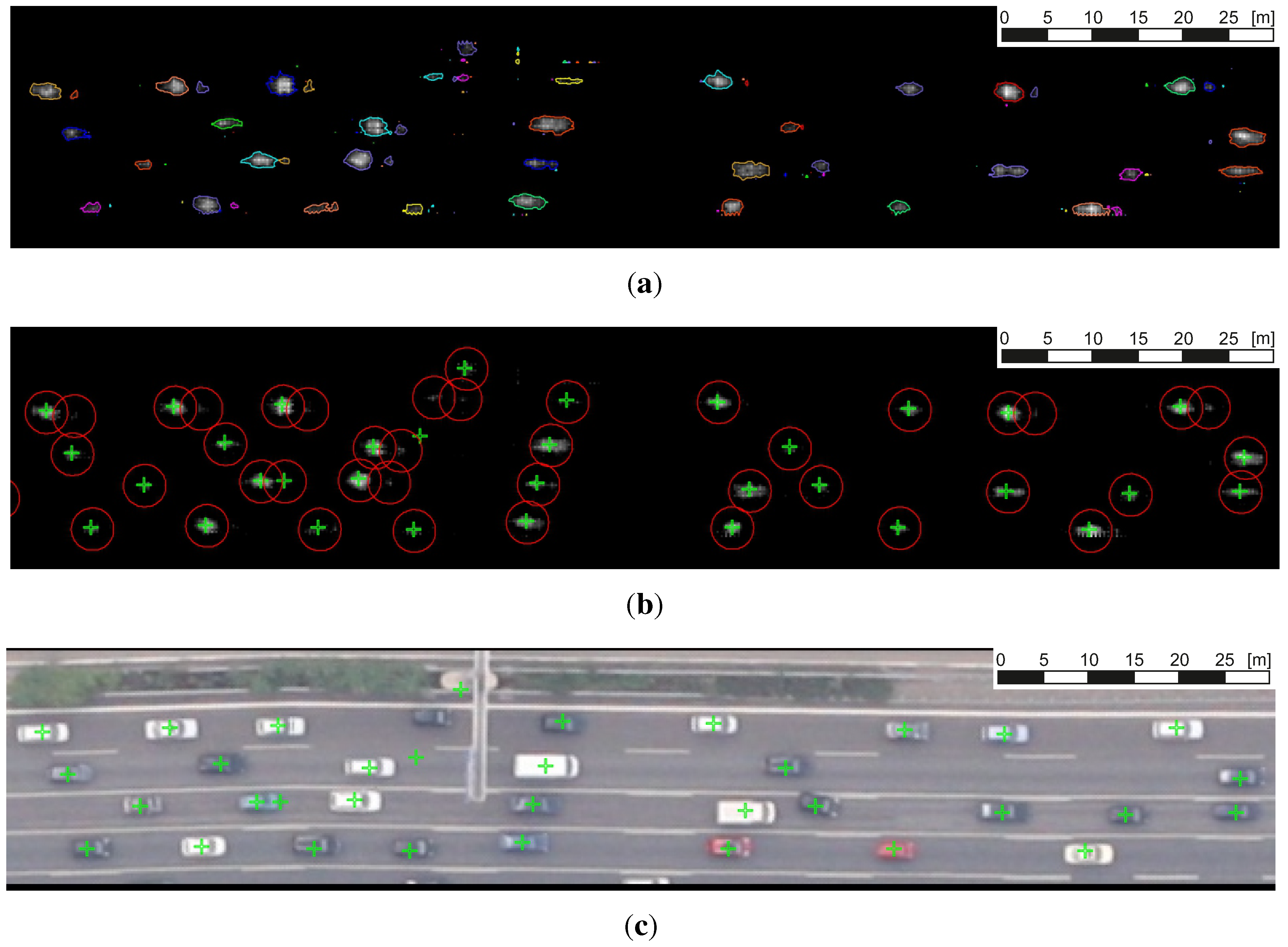
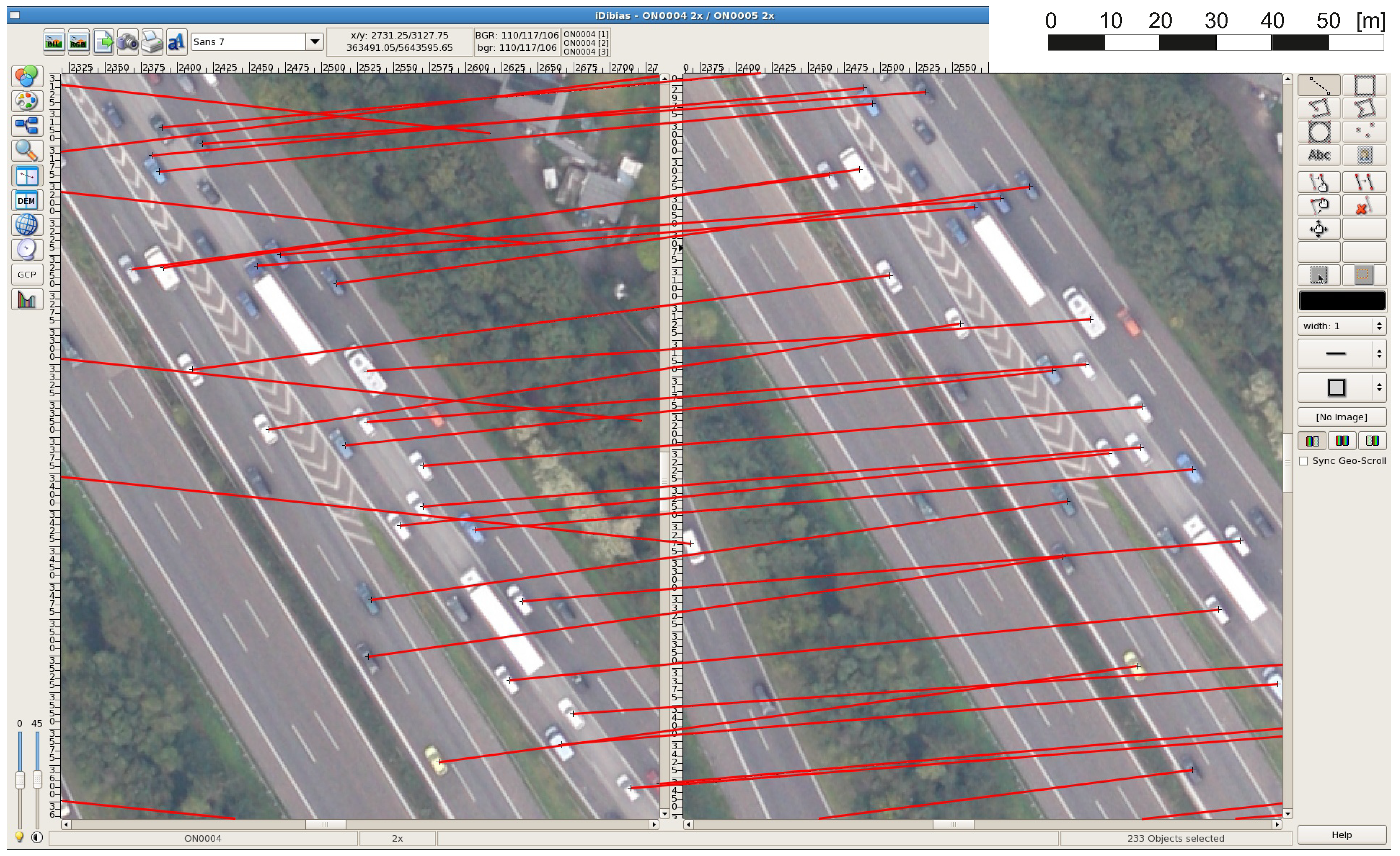
In order to speed up the search, a hierarchical search using image pyramids is used. Figure 5 shows the typical result obtained from the vehicle matching operator prior to the elimination of outliers. The vehicle positions obtained after tracking are stored and can be used for a second call of the vehicle tracking module with the next image pair of the sequence.

The first step in reducing outliers is performed in the vehicle tracking module inside the aircraft. The goal is to reduce false matches in tracking, as well as false positives in detection (e.g., road markings that have been erroneously detected as vehicles). The latter may be partially revealed by a possible irregular behavior in tracking. If the direction deviation exceeds 30°, the match is refused. No direction criterion is applied below a speed threshold of 10 km/h, since inaccuracies in georeferencing may influence travel directions beyond the derivation criterion (see also Section 5.3). The threshold value of 30° was chosen, since we already observed angles of more than 20° during lane changes in the case of congestion situations on motorways. Moreover, in intersection areas, we observed vehicles with up to a 30° deviation from the straight driving direction, which need to be detected by our rotation variant vehicle detector (Section 3.2). ASCII data files containing the corrected tracking results are transferred to the ground instantaneously via a radio link system. Since the radio link may be working at full capacity due to the images being sent to the ground, ASCII files with traffic data are highly prioritized in order to keep the traffic data highly current.

Further outlier reduction is performed on the ground due to limited processing power on-board the aircraft. A fuzzy logic is applied for this purpose, as described in [42]. In summary, vehicle velocities are evaluated with respect to the state of traffic and the distance to or from the next intersection. For example, if a vehicle is far from an intersection and its velocity is significantly below the average of the free flowing traffic situation around the car, it is rejected. If the image burst sequence consists of more than two consecutive images, a further validation of plausibility for each vehicle trajectory is performed at the ground station. The time derivatives of velocity and direction are checked for plausibility for each vehicle track. If the acceleration, deceleration or direction change leaves physically realistic value ranges, the vehicle trajectory is assumed to be an outlier and removed from the traffic data. The thresholds for the maximum acceleration and deceleration allowed are set to 5 m/s² and 10 m/s². The maximum acceleration is a typical value for a premium car, like the Porsche Cayenne Turbo or Jaguar XKR Coupe (0–100 km/h) [82]. The maximum deceleration is a typical value for a premium car (e.g., Mercedes CLK 430 or Chevrolet Corvette, 100–0 km/h) [82]. For direction change, a maximum of 8°/s (0.1396 rad/s) is allowed. This value is due to the following assumptions. The minimum curve radius for European motorways with a recommended speed of 80 km/h is 240 m (e.g., [83]). This corresponds to a lateral acceleration of 2 m/s². In [84], the measured velocity v_85% in bends with a radius of 240 m is 92 km/h is shown. This corresponds to a lateral acceleration of 2.8 m/s². In order to additionally catch the 15% of drivers driving faster than 92 km/h, we assume an additional 20% and an additionally constant of 10 km/h for the 92 km/h, as described before. Totally, we assume for a bend with a 240-m radius a maximum speed of 120 km/h. This value leads to a rate of turn of 7.95°/s, which we rounded to 8°/s. This corresponds to a lateral acceleration of 4.6 m/s².

At the ground station, traffic data obtained by the airborne camera system are prepared for use in a traffic portal or GIS. This is done by assigning each vehicle to its nearest Navteq road section while taking into account that its driving direction has to correspond to the direction of the respective Navteq section. If the vehicle cannot be allocated to any road axis, it is assumed to be an outlier and rejected. This outlier correction does not influence the behavior of the traffic data extraction at intersections. This is due to the following fact. Since the vehicle detector is sensitive to driving directions, we cannot detect vehicles which have a direction angle of more than around 30°/s for any Navteq road axis. Nevertheless, vehicles lost due to this property of the vehicle detector are rare in practice. An average vehicle density and velocity is calculated for each Navteq segment located in the first image of a burst. This spatially aggregated data represent the road level-of-service. Single vehicle trajectories can be used after fusion with the traffic information recorded by ground-based sensor networks for the initialization of traffic simulations (e.g., [14]).

Figure 5. Typical matching result of the vehicle tracking algorithm between the first (left) and second image (right) of a camera burst (example from the nadir camera, Cologne campaign on 17 September 2011).

Figure 5. Typical matching result of the vehicle tracking algorithm between the first (left) and second image (right) of a camera burst (example from the nadir camera, Cologne campaign on 17 September 2011).

4. Datasets

4.1. Training and Reference Data

All in all, more than 4700 vehicles have been manually extracted from images of previous campaigns and test flights. All of the images have been sampled to a 0.20-m ground sampling distance. To obtain a large number of samples for the background class (negative examples), large road areas without vehicles on it were marked manually. Within those areas, samples were extracted at random positions. We set the number of background samples to 15,000 to have a good ratio between the number of training samples of the vehicle and background class.

4.2. Campaign

In the past few years, the traffic monitoring system has been tested on several test flights and campaigns in Munich and Cologne. For instance, it was flown during the BAUMAexhibition (World’s Leading International Trade Fair for Construction Machinery, Building Material Machines, Mining Machines, Construction Vehicles and Construction Equipment) on 22 April and 24 April 2010, at the Munich Exhibition Center and the skirting motorway A 94. The flight height of this campaign was 1000 m above ground. Further campaigns were flown in Cologne on 2 June 2009, at a flight height of 1500 m and during Aerospace Day in Cologne on 18 September 2011. The results of an extensive system test prior to Aerospace Day on 17 September 2011, are shown in Section 5. Images were taken at flight levels of 1200 m and 1500 m above ground (depending on air space control permission) on motorways and main roads in Cologne. They were orthorectified with a GSD of 0.2 m, since the complete system and the vehicle detector are only configured for this resolution. Image sequences were acquired in triple bursts with an intermission of 0.7 s between consecutive images within a burst. The break between the last image of a given burst and the first image of its subsequent burst was 5.5 s.

During summer, 2011, the 3K system was exchanged with the 3K+ system. Thus, data for the BAUMA campaign in 2010 and Cologne in 2009 were taken with the 3K system, while the second campaign in Cologne from 2011 was flown with the 3K+ system.

5. Results

For the evaluation of the vehicle detection and tracking algorithms, the values for correctness, completeness and quality are calculated for different scenes from several campaigns. They are defined as:

$$Correctness(Compl.)\text{\hspace{0.17em}=\hspace{0.17em}}\frac{truepositives}{truepositives+falsepositives}$$

(6)

$$Completeness(Corr.)\text{\hspace{0.17em}=\hspace{0.17em}}\frac{truepositives}{truepositives+falsenegatives}$$

(7)

$$Quality(Qual.)\text{\hspace{0.17em}=\hspace{0.17em}}\frac{truepos}{truepos+falsepos+falseneg}$$

(8)

with true positives being the number of vehicles detected, false positives the number of non-vehicle detections and false negatives the number of vehicles missed. In the tracking evaluation, true positives is the number of vehicles tracked correctly, false positives the number of incorrectly tracked vehicles and false negatives the number of vehicles detected, but not tracked (vehicles that are not tracked during image bursts due to occlusion are not counted as false positives). In total, 104 images from several campaigns were evaluated for detection quality. For the tracking, 104 image bursts were examined. The quality value here is considered to be the strictest criterion, since it contains both possible detection errors, namely false positives and false negatives.

Figure 6 shows a typical result of the traffic extraction. It was obtained online and in real time during the Cologne campaign on 17 September 2011 (3K+), at the three-leg interchange “Heumar”. The correctness, completeness and quality values of the vehicle detection are 98.2%, 86.6% and 85.2% in this specific scene. The correctness, completeness and quality parameters of the tracking result obtained from that scene are 96.8%, 98.1% and 95.1%.

5.1. Results of Vehicle Detection

Vehicle detection was validated manually. In each first image of a burst, the number of false detections and non-detections was counted. Table 2 shows the evaluation result of the vehicle detection on a dataset from Cologne in 2009 (3K system). It contains a mix of suburban, motorway and urban core scenes. The average quality of the Cologne 2009 detection results was 83%. During the BAUMA 2010 campaign in Munich (3K system), the average quality of vehicle detection was 86% (Table 3). In the Cologne 2011 campaign, which took place in mixed weather conditions, the total quality of the detection was 77% (Table 4). The top image in Figure 7 shows the limitations of the original detector in a complex scene. This image shows the maximum outlier of the detection quality during the campaign. The cables of the bridge result in a higher number of false positives due to the fact that the Haar-like features are very sensitive strong edges. There are also false detections in the case of vehicle-like objects, e.g., shadows of road signs or marked parking lots, which have similar dimensions as cars. To improve the detection rate, the results are checked visually after the end of the campaign. If there seem to be many errors, vehicles and their tracks are manually acquired and used for re-training the classifiers. The false positives were used as new/additional negatives examples. In the lower image of Figure 7, the results after the retraining process can be seen. The quality of the data obtained in the scene has been improved significantly.

Figure 6. Typical result of the traffic data extraction obtained online during the Cologne campaign 2011 (3K+ system). It shows traffic congestion at the “Heumar” three-leg interchange. Vehicle velocities are color coded.

Figure 6. Typical result of the traffic data extraction obtained online during the Cologne campaign 2011 (3K+ system). It shows traffic congestion at the “Heumar” three-leg interchange. Vehicle velocities are color coded.

Table 2. Evaluation of vehicle detection quality on Cologne 2009 data (3K system).

Scene	Suburban & Motorways	Urban Core	Total
Images evaluated	73	6	79
True Positives	5545	2911	8456
False Positives	613	429	1042
False Negatives	424	317	741
Correctness	90%	87%	89%
Completeness	93%	90%	92%
Quality	84%	80%	83%

Table 2. Evaluation of vehicle detection quality on Cologne 2009 data (3K system).

Scene	Suburban & Motorways	Urban Core	Total
Images evaluated	73	6	79
True Positives	5545	2911	8456
False Positives	613	429	1042
False Negatives	424	317	741
Correctness	90%	87%	89%
Completeness	93%	90%	92%
Quality	84%	80%	83%

Table 3. Evaluation of vehicle detection quality on BAUMA2010 data at Munich (3K system).

	True	False	False	Compl.	Corr.	Qual.
	Positives	Positives	Negatives	(%)	(%)	(%)
BAUMA1	1221	39	90	93.1	96.9	90.4
BAUMA2	743	9	134	84.7	98.8	83.9
Total	1953	48	224	89.7	95.6	86.1

Table 3. Evaluation of vehicle detection quality on BAUMA2010 data at Munich (3K system).

	True	False	False	Compl.	Corr.	Qual.
	Positives	Positives	Negatives	(%)	(%)	(%)
BAUMA1	1221	39	90	93.1	96.9	90.4
BAUMA2	743	9	134	84.7	98.8	83.9
Total	1953	48	224	89.7	95.6	86.1

Table 4. Evaluation of vehicle detection quality on Cologne 2011 data (3K+ system).

	True	False	False	Compl.	Corr.	Qual.
	Positives	Positives	Negatives	(%)	(%)	(%)
Detection	1741	356	165	91.3	83.0	77.0

Table 4. Evaluation of vehicle detection quality on Cologne 2011 data (3K+ system).

	True	False	False	Compl.	Corr.	Qual.
	Positives	Positives	Negatives	(%)	(%)	(%)
Detection	1741	356	165	91.3	83.0	77.0

Figure 7. (Top) Results of original vehicle detection on a complex bridge scene that resulted in a low quality of 48% (Cologne campaign 2011 with 3K+ system). (Bottom) Results of vehicle detection on the same scene after retraining the AdaBoost classifier.

Figure 7. (Top) Results of original vehicle detection on a complex bridge scene that resulted in a low quality of 48% (Cologne campaign 2011 with 3K+ system). (Bottom) Results of vehicle detection on the same scene after retraining the AdaBoost classifier.

5.2. Results of Vehicle Tracking

Campaign vehicle tracking was evaluated manually in three steps on each first and second image of an image burst. First, the number of detected cars that can be tracked was determined. This is the number of cars that were not occluded in consecutive image pairs. This number is typically lower than the number of detected cars, since the overlap between the first and second image of an image burst is usually less than 100%. Vehicles outside the overlap region cannot be tracked. Furthermore, there are few vehicles that are detected in the first image, but occluded by other image objects in the second image. These vehicles also cannot be tracked. The loss of vehicles in tracking due to the image overlap of consecutive images within a burst could be compensated for by increasing the overlap of image bursts. Subsequently, the number of false positives (i.e., the number of vehicles that were incorrectly tracked) and false detections were counted.

Table 5 shows the results of the tracking evaluation for the BAUMA campaign. The results of the tracking were quite good with high values of completeness (97%), correctness (93%) and quality (91%). On motorway scenes with image sequences taken in good weather conditions, tracking seemed to work fine. In Table 6, the results of the tracking evaluation of the Cologne campaign 2011, which took place under unfavorable weather conditions, are shown. The scenes include a mixture of images of downtown, suburban areas and rural motorways. In this case, an average completeness of 92%, a correctness of 94% and a quality of 88% were obtained. The minimum value of quality observed in two scenes was 71%. In one of these scenes, the exposures were foggy. Based on these results, the tracking algorithm shows a good performance, even in complex scenes. Vehicle tracking performed best on the Cologne 2009 campaign (Table 7). There, the values for correctness, completeness and quality were 97%, 96% and 93%.

Table 5. Evaluation of vehicle tracking quality based on BAUMA 2010 data in Munich (3K system).

Campaign	BAUMA 1	BAUMA 2	Total
Bursts evaluated	29	19	48
True Positives	1002	724	1726
False Positives	75	47	122
False Negatives	36	23	59
Correctness	93%	94%	93%
Completeness	97%	97%	97%
Quality	90%	91%	91%

Table 5. Evaluation of vehicle tracking quality based on BAUMA 2010 data in Munich (3K system).

Campaign	BAUMA 1	BAUMA 2	Total
Bursts evaluated	29	19	48
True Positives	1002	724	1726
False Positives	75	47	122
False Negatives	36	23	59
Correctness	93%	94%	93%
Completeness	97%	97%	97%
Quality	90%	91%	91%

Table 6. Evaluation of vehicle tracking quality on Cologne 2011 data (3K+ system).

	True	False	False	Compl.	Corr.	Qual.
	Positives	Positives	Negatives	(%)	(%)	(%)
Tracking	1125	62	92	92.4	94.8	88.0

Table 6. Evaluation of vehicle tracking quality on Cologne 2011 data (3K+ system).

	True	False	False	Compl.	Corr.	Qual.
	Positives	Positives	Negatives	(%)	(%)	(%)
Tracking	1125	62	92	92.4	94.8	88.0

Table 7. Evaluation of vehicle tracking quality based on Cologne 2009 data (3K system).

Scene	Suburban & Motorways	Urban Core	Total
Bursts evaluated	49	5	54
True Positives	2654	2050	4704
False Positives	85	58	143
False Negatives	118	88	206
Correctness	97%	97%	97%
Completeness	96%	96%	96%
Quality	93%	93%	93%

Table 7. Evaluation of vehicle tracking quality based on Cologne 2009 data (3K system).

Scene	Suburban & Motorways	Urban Core	Total
Bursts evaluated	49	5	54
True Positives	2654	2050	4704
False Positives	85	58	143
False Negatives	118	88	206
Correctness	97%	97%	97%
Completeness	96%	96%	96%
Quality	93%	93%	93%

Figure 8 shows the result of tracking in the case of a thin cloud coming into the line of sight between the first and second image of the camera burst. Although the second exposure is slightly covered by that cloud, tracking performs well.

Figure 8. Matching result of the vehicle tracking algorithm between the first (left) and second image (right) of a camera burst in the case of thin clouds (Cologne campaign 2011 with the 3K+ system).

Figure 8. Matching result of the vehicle tracking algorithm between the first (left) and second image (right) of a camera burst in the case of thin clouds (Cologne campaign 2011 with the 3K+ system).

5.3. Overall Accuracy

Individual vehicles have a positioning error that is around a factor of 10 less than their size (RMSEs of the X Y -position range from 0.14 m to 0.38 m; please refer to [10]). The velocity accuracy of a single vehicle tracked using aerial image sequences of this 3K camera system was examined in [85]. It was found to be below 5 km/h. The uncertainty of moving direction is dependent on the driving velocity. It is mainly influenced by the positioning error due to the direct georeferencing procedure. For a vehicle with a velocity of 10 km/h, it may exceed 30° in the extreme case. At a speed of 100 km/h, it is typically less than 4°.

The overall accuracy of derived traffic densities depends on the completeness, correctness and quality of the detection. Our detection quality is in the range of 78% (Cologne campaign in 2011) and 86% (in 2010). A comparison of aerial image-based detection errors and stationary ground detectors, such as induction loop detectors or traffic cams, is challenging due to the different species of data obtained (ground sensors deliver punctual information, whereas aerial images provide area-wide data with a low time resolution). However, the over-count rate of a highway network is comparable to the false positive rates obtained by our vehicle detection. In [86], the over-count rate of induction loops of a freeway in Portland, USA, was found to be 8.3%. In comparison, the correctness of our car detection algorithm was evaluated to be around 90% in suburban regions (Table 2). This corresponds to an over-count rate of 10%. The detection rate of induction loops straight from the factory varies between 90% and 97% [87]. The completeness of our detection is in the range of 90% to 92%, depending on the complexity of the scene (higher in scenes with lower complexity, like motorways or highways). As induction loops age, their quotas decrease. However, the quota of our system is not dependent on aging effects.

The completeness of our tracking is in the range of 92% to 97% (Cologne 2011 and BAUMA Campaign 2010), which means that 92% to 97% of the vehicles detected were tracked properly. Overall system completeness, including detection and tracking, is expressed as the detection completeness times the tracking completeness. In our case, we end up with a system completeness in the range of 68% (Cologne 2011) to 81% (BAUMA1 in 2010). In order to measure the velocity of a specific car with induction loops, it must produce a detection in two consecutive induction loops. With each induction loop having a completeness of 90% to 97%, the system completeness for measuring velocities from induction loops is between 81% and 94%. Such dual loop detectors may also produce some false positives. In [88], it is stated that dual loop sensors tend to underestimate the bin volumes, although overestimation errors occur occasionally. In cases of false positives, the correctness of the data delivered can drop to a value of 53%. In comparison, the correctness of our system is expressed as the detection correctness times the tracking correctness and lies between 68% and 81%. The quality of our airborne-generated traffic information therefore touches the quality range of induction loop networks, with the advantage that our system provides a higher spatial coverage.

5.4. Performance

The processing chain for traffic monitoring on the on-board hardware used is real-time capable. This means that an image burst consisting of three images for each camera’s looking direction can be processed and analyzed by the processing chain before the recording of the next burst has been finished. With respect to Section 4.2, total processing times for each burst must not exceed 7 s. These benchmark tests have been performed with a maximum of 1000 vehicles in the scenes. We assume that this is the absolute maximum number of vehicles to be found in an image scene of one looking direction (e.g., in downtown areas of large metropolises). In this case, the computing time for vehicle detection module is 2.5 s, and for the tracking module is 2.1 s on the given on-board hardware. With only a few cars in the image scene, the processing time decreases to values of around 1 s for each module. As stated before, georeferencing and orthorectification are processed at the GPU with typical processing times of 250 ms for each image. This performance allows us to process images just in time without accumulating a stack of unprocessed images during operating time. A prioritization of traffic data with respect to image data during the downlinking process makes it possible to deliver current traffic data to the ground with a maximum delay of 7 s or less in the case of the microwave downlink system. In the case of the laser link terminal, the data bandwidth is not a concern.

6. Conclusions

We propose a solution for automatic extraction of traffic information from airborne images, which satisfies the increasing demand for accurate and actual traffic data. Thereby, the system maturity has reached an operational state, which is shown by the system validation performed based on data obtained during several missions with varying conditions. We obtain aerial image sequences that are fully automatically analyzed for road traffic content. The analysis is divided into a detection and a tracking part. In the detection part, a combination of the machine learning algorithms Adaboost and SVM detects vehicle objects with an average detection quality ranging from 78% in poor weather to 91% in good weather conditions. During the tracking part, template matching of vehicle objects detected before is done with a following plausibility check of resulting trajectories. In tracking, an average quality of 88% to 93% is reached during several campaigns. The whole processing chain from image acquisition to distribution to end-users is performed in real time on-board the aircraft and on the ground. Traffic data is brought into the Internet traffic portal with a delay of less than 7 s. This ensures that the traffic data provided are highly up-to-date. It was shown that the system’s accuracy is almost on par with that of ground stationary sensor systems. Nevertheless, it turns out that the quality of the traffic data obtained by our system can be increased with additional detector training. Since our system is independent of any stationary ground infrastructure, it can be used in cases where no ground infrastructure is available. This could occur during mass events (if they take place at locations beyond any sensor networks) or disaster situations (if ground sensor networks are affected). Since the system has the ability to collect traffic data on all kinds of road categories, it can be used as an additional data source for conurbation areas. For example, it could be applied in case studies, traffic census or traffic light phase optimization. Although the operational qualities of the system have been proven in this work, some improvements could be made. In the actual processing chain, the positions of detected vehicles are allocated to Navteq segments. A more precise allocation of vehicle positions, not only to road sections, but also to traffic lanes, would enhance the resolution of traffic simulation. However, the Navteq data does not provide exact information on traffic lanes. Therefore, the focus of future work will be on lane-specific traffic extraction in order to enhance the data input for traffic simulations. Moreover, vehicle classes (cars and trucks) will be distinguished by the employment of two different vehicle detectors. With a future miniaturization of the system hardware, small aircraft and helicopters as platforms with low operating costs will be feasible.

References

1. Schӓfer, R.; Thiessenhusen, K.; Wagner, P. A traffic information system by means of real-time floating-car data. In Proceedings of the ITS World Congress, Chicago, IL, USA, 11–14 October 2002; Volume 2.
2. Lorkowski, S.; Brockfeld, E.; Mieth, P.; Passfeld, B.; Thiessenhusen, K.; Schӓfer, R.; für Luft, D. Erste Mobilitӓtsdienste auf Basis von “Floating Car Data”. Available online: http://elib.dlr.de/6613/1/Vortrag.pdf (accessed on 7 November 2014).
3. Busch, F.; Glas, F.; Bermann, E. Dispositionssysteme als FCD-Quellen für eine verbesserte Verkehrslagerekonstruktion in Stӓdten. Straßenverkehrstechnik 2004, 9, 437–444. [Google Scholar]
4. Geisler, S.; Chen, Y.; Quix, C.; Gehlen, G. Accuracy assessment for traffic information derived from floating phone data. In Proceedings of the Intelligent Transportation Systems and Services World Congress, Busan, Korea, 25–29 October 2010.
5. Brockfeld, E.; Lorkowski, S.; Mieth, P.; Wagner, P. Benefits and limits of recent floating car data technology—An evaluation study. In Proceedings of the 11th WCTR Conference, Berkeley, CA, USA, 24–28 June 2007; pp. 24–28.
6. Ernst, I.; Sujew, S.; Thiessenhusen, K.; Hetscher, M.; Rassmann, S.; Ruhe´, M. LUMOS-airborne traffic monitoring system. In Proceedings of the 2003 Intelligent Transportation Systems, Shanghai, China, 12–15 October 2003; Volume 1, pp. 753–759.
7. Börner, A.; Ernst, I.; Ruhe´, M.; Sujew, S.; Hetscher, M. Airborne camera experiments for traffic monitoring. Int. Arch. Photogramm. Remote Sens. Spat. Inf. Sci. 2004, 35, 243–248. [Google Scholar]
8. Rosenbaum, D.; Charmette, B.; Kurz, F.; Suri, S.; Thomas, U.; Reinartz, P. Automatic traffic monitoring from an airborne wide angle camera system. Int. Arch. Photogramm. Remote Sens. Spat. Inf. Sci. 2008, 37, 557–562. [Google Scholar]
9. Baumgartner, S.; Krieger, G. A priori knowledge based GMTI algorithm for traffic monitoring applications. In Proceedings of the 2010 8th European Conference on Synthetic Aperture Radar (EUSAR 2010), Aachen, Germany, 7–10 June 2010; pp. 1–4.
10. Kurz, F.; Türmer, S.; Meynberg, O.; Rosenbaum, D.; Leitloff, J.; Runge, H.; Reinartz, P. Low-cost optical camera systems for real time mapping applications. Photogramm. Fernerkund. Geoinf. 2012, 2012, 159–176. [Google Scholar]
11. Horwath, J.; Fuchs, C. Aircraft to ground unidirectional laser-communications terminal for high-resolution sensors. Proc. SPIE 2009. [Google Scholar] [CrossRef]
12. Römer, H.; Kersten, J.; Kiefl, R.; Plattner, S.; Mager, A.; Voigt, S. Airborne near-real-time monitoring of assembly and parking areas in case of large-scale public events and natural disasters. Int. J. Geogr. Inf. Sci. 2014, 28, 682–699. [Google Scholar] [CrossRef]
13. Frassl, M.; Lichtenstern, M.; Khider, M.; Angermann, M. Developing a system for information management in disaster relief—Methodology and requirements. In Proceedings of the 7th International ISCRAM Conference, Seattle, WA, USA, 2–5 May 2010.
14. Behrisch, M.; Bonert, M.; Brockfeld, E.; Krajzewicz, D.; Wagner, P. Event traffic forecast for metropolitan areas based on microscopic simulation. In Proceedings of the Third International Symposium of Transport Simulation 2008 (ISTS08), Surfers Paradise, QLD, Australia, 6–8 August 2008.
15. Thomas, U.; Rosenbaum, D.; Kurz, F.; Suri, S.; Reinartz, P. A new software/hardware architecture for real time image processing of wide area airborne camera images. J. Real-Time Image Process. 2009, 4, 229–244. [Google Scholar]
16. Stilla, U.; Michaelsen, E.; Sörgel, U.; Hinz, S.; Ender, J. Airborne monitoring of vehicle activity in urban areas. Int. Arch. Photogramm. Remote Sens. Spat. Inf. Sci. 2004, 35, 973–979. [Google Scholar]
17. Hinz, S.; Bamler, R.; Stilla, U. Theme issue: “Airborne and spaceborne traffic monitoring”. ISPRS J. Photogramm. Remote Sens. 2006, 61, 135–136. [Google Scholar] [CrossRef]
18. Ramakrishnan, V.; Kethsy Prabhavathy, A.; Devishree, J. A survey on vehicle detection techniques in aerial surveillance. Int. J. Comput. Appl. 2012, 55, 43–47. [Google Scholar]
19. Burlina, P.; Parameswaran, V.; Chellappa, R. Sensitivity analysis and learning strategies for context-based vehicle detection algorithms. In Proceedings of the DARPA Image Understanding Workshop, New Orleans, LA, USA, 11–14 May 1997; pp. 577–584.
20. Moon, H.; Chellappa, R.; Rosenfeld, A. Performance analysis of a simple vehicle detection algorithm. Image Vis. Comput. 2002, 20, 1–13. [Google Scholar] [CrossRef]
21. Zhao, T.; Nevatia, R. Car detection in low resolution aerial images. Image Vis. Comput. 2003, 21, 693–703. [Google Scholar] [CrossRef]
22. Hinz, S. Detection of vehicles and vehicle queues in high resolution aerial images. Photogramm. Fernerkund. Geoinf. 2004, 3, 201–213. [Google Scholar]
23. Ruskone´, R.; Guiges, L.; Airault, S.; Jamet, O. Vehicle detection on aerial images: A structural approach. In Proceedings of the 13th International Conference on Pattern Recognition, Vienna, Austria, 25–29 August 1996; Kropatsch, G., Ed.; IEEE Computer Society Press: Vienna, Austria, 2004; Volume 3, pp. 900–903. [Google Scholar]
24. Spiegel, M. Automatische Erkennung von Fahrzeugen aus digitalen Luftbildern mittels Neuronaler Netze. Master’s Thesis, Technische Universitӓt München, Munich, Germany, 2000. [Google Scholar]
25. Grabner, H.; Nguyen, T.T.; Gruber, B.; Bischof, H. On-line boosting-based car detection from aerial images. ISPRS J. Photogramm. Remote Sens. 2008, 63, 382–396. [Google Scholar] [CrossRef]
26. Kembhavi, A.; Harwood, D.; Davis, L.S. Vehicle detection using partial least squares. IEEE Trans. Pattern Anal. Mach. Intell. 2011, 33, 1250–1265. [Google Scholar] [CrossRef] [PubMed]
27. Türmer, S.; Kurz, F.; Reinartz, P.; Stilla, U. Airborne vehicle detection in dense urban areas using HoG features and disparity maps. IEEE J. Sel. Top. Appl. Earth Observ. Remote Sens. 2013, 6, 2327–2337. [Google Scholar] [CrossRef]
28. Dalal, N.; Triggs, B. Histograms of oriented gradients for human detection. In Proceedings of the 2005 IEEE Computer Society Conference on Computer Vision and Pattern Recognition (CVPR 2005), San Diego, CA, USA, 20–26 June 2005; Volume 1, pp. 886–893.
29. Gaszczak, A.; Breckon, T.P.; Han, J. Real-time people and vehicle detection from UAV imagery. In Proceedings of the IS&T/SPIE Electronic Imaging. International Society for Optics and Photonics, San Fransico, CA, USA, 23 January 2011.
30. Gleason, J.; Nefian, A.; Bouyssounousse, X.; Fong, T.; Bebis, G. Vehicle detection from aerial imagery. In Proceedings of the 2011 IEEE International Conference on Robotics and Automation (ICRA 2011), Shanghai, China, 9–13 May 2011; pp. 2065–2070.
31. Reilly, V.; Solmaz, B.; Shah, M. Shadow Casting Out Of Plane (SCOOP) candidates for human and vehicle detection in aerial imagery. Int. J. Comput. Vis. 2013, 101, 350–366. [Google Scholar] [CrossRef]
32. Moranduzzo, T.; Melgani, F. Detecting cars in UAV images with a catalog-based approach. IEEE Trans. Geosci. Remote Sens. 2014, 52, 6356–6367. [Google Scholar] [CrossRef]
33. Kurz, F.; Meynberg, O.; Rosenbaum, D.; Türmer, S.; Reinartz, P.; Schroeder, M. Low-cost optical camera system for disaster monitoring. Int. Arch. Photogramm. Remote Sens. Spat. Inf. Sci. 2012, 39, 33–37. [Google Scholar] [CrossRef]
34. Dreschler, L.; Nagel, H.H. Volumetric model and 3-D trajectory of a moving car derived from monocular TV frame sequences of a street scene. Comput. Graph. Image Process. 1982, 20, 199–228. [Google Scholar] [CrossRef]
35. Haag, M.; Nagel, H.H. Combination of edge element and optical flow estimates for 3D-model-based vehicle tracking in traffic image sequences. Int. J. Comput. Vis. 1999, 35, 295–319. [Google Scholar] [CrossRef]
36. Jolly, M.P.D.; Lakshmanan, S.; Jain, A.K. Vehicle segmentation and classification using deformable templates. IEEE Trans. Pattern Anal. Mach. Intell. 1996, 18, 293–308. [Google Scholar] [CrossRef]
37. Tan, T.N.; Sullivan, G.D.; Baker, K.D. Model-based localisation and recognition of road vehicles. Int. J. Comput. Vis. 1998, 27, 5–25. [Google Scholar] [CrossRef]
38. Lachaise, M. Automatic Detection of Vehicles and Velocities in Aerial Digital Image Series. Master’s Thesis, Ecole Superieure de Chimie Physique Electronique de Lyon, Lyon, France, 2005. [Google Scholar]
39. Reinartz, P.; Lachaise, M.; Schmeer, E.; Krauss, T.; Runge, H. Traffic monitoring with serial images from airborne cameras. ISPRS J. Photogramm. Remote Sens. 2006, 61, 149–158. [Google Scholar] [CrossRef]
40. Kozempel, K.; Reulke, R. Fast vehicle detection and tracking in aerial image bursts. Int. Arch. Photogramm. Remote Sens. Spat. Inf. Sci. 2009, 38, 175–180. [Google Scholar]
41. Lenhart, D.; Hinz, S.; Leitloff, J.; Stilla, U. Automatic traffic monitoring based on aerial image sequences. Pattern Recogn. Image Anal. 2008, 18, 400–405. [Google Scholar] [CrossRef]
42. Butenuth, M.; Reinartz, P.; Lenhart, D.; Rosenbaum, D.; Hinz, S. Analysis of image sequences for the detection and monitoring of moving traffic. Photogramm. Fernerkund. Geoinf. 2009, 2009, 421–430. [Google Scholar] [CrossRef]
43. Cao, X.; Shi, Z.; Yan, P.; Li, X. Collaborative Kalman filters for vehicle tracking. In Proceedings of the 2011 IEEE International Workshop on Machine Learning for Signal Processing (MLSP 2011), Beijing, China, 18–21 September 2011; pp. 1–6.
44. Szottka, I.; Butenuth, M. Advanced particle filtering for airborne vehicle tracking in urban areas. IEEE Geosci. Remote Sens. Lett. 2014, 11, 686–690. [Google Scholar] [CrossRef]
45. Zheng, H.; Pan, L.; Li, L. A morphological neural network approach for vehicle detection from high resolution satellite imagery. In Neural Information Processing; Springer: Berlin/Heidelberg, Germany, 2006; pp. 99–106. [Google Scholar]
46. Jin, X.; Davis, C.H. Vehicle detection from high-resolution satellite imagery using morphological shared-weight neural networks. Image Vis. Comput. 2007, 25, 1422–1431. [Google Scholar] [CrossRef]
47. Eikvil, L.; Aurdal, L.; Koren, H. Classification-based vehicle detection in high-resolution satellite images. ISPRS J. Photogramm. Remote Sens. 2009, 64, 65–72. [Google Scholar] [CrossRef]
48. Leitloff, J.; Hinz, S.; Stilla, U. Vehicle detection in very high resolution satellite images of city areas. IEEE Trans. Geosci. Remote Sens. 2010, 48, 2795–2806. [Google Scholar] [CrossRef]
49. Larsen, S.Ø.; Salberg, A.B.; Eikvil, L. Automatic system for operational traffic monitoring using very-high-resolution satellite imagery. Int. J. Remote Sens. 2013, 34, 4850–4870. [Google Scholar] [CrossRef]
50. Leitloff, J.; Hinz, S.; Stilla, U. Inferring traffic activity from optical satellite images. In Proceedings of the Photogrammetric Image Analysis (PIA07), Munich, Germany, 19–21 September 2007; pp. 89–93.
51. Salehi, B.; Zhang, Y.; Zhong, M. Automatic moving vehicles information extraction from single-pass WorldView-2 imagery. IEEE J. Sel. Top. Appl. Earth Observ. Remote Sens. 2012, 5, 135–145. [Google Scholar] [CrossRef]
52. Gao, F.; Li, B.; Xu, Q.; Zhong, C. Moving vehicle information extraction from single-pass WorldView-2 imagery based on ERGAS-SNS analysis. Remote Sens. 2014, 6, 6500–6523. [Google Scholar] [CrossRef]
53. Yao, W.; Hinz, S.; Stilla, U. Extraction and motion estimation of vehicles in single-pass airborne LiDAR data towards urban traffic analysis. ISPRS J. Photogramm. Remote Sens. 2011, 66, 260–271. [Google Scholar] [CrossRef]
54. Yao, W.; Zhang, M.; Hinz, S.; Stilla, U. Airborne traffic monitoring in large areas using LiDAR data—Theory and experiments. Int. J. Remote Sens. 2012, 33, 3930–3945. [Google Scholar] [CrossRef]
55. Borcs, A.; Benedek, C. Extraction of vehicle groups in airborne Lidar point clouds with two-level point processes. IEEE Trans. Geosci. Remote Sens. 2015, 53, 1475–1489. [Google Scholar] [CrossRef]
56. Meyer, F.; Hinz, S.; Laika, A.; Weihing, D.; Bamler, R. Performance analysis of the TerraSAR-X traffic monitoring concept. ISPRS J. Photogramm. Remote Sens. 2006, 61, 225–242. [Google Scholar] [CrossRef]
57. Budillon, A.; Pascazio, V.; Schirinzi, G. Estimation of radial velocity of moving targets by along-track interferometric SAR systems. IEEE Geosci. Remote Sens. Lett. 2008, 5, 349–353. [Google Scholar] [CrossRef]
58. Guo, B.; Vu, D.; Xu, L.; Xue, M.; Li, J. Ground moving target indication via multichannel airborne SAR. IEEE Trans. Geosci. Remote Sens. 2011, 49, 3753–3764. [Google Scholar] [CrossRef]
59. Yao, W.; Hinz, S.; Stilla, U. Automatic analysis of traffic scenario from airborne thermal infrared video. Int. Arch. Photogramm. Remote Sens. Spat. Geoinf. Sci. 2008, 37, 223–228. [Google Scholar]
60. Baumgartner, S.V.; Krieger, G. Fast GMTI algorithm for traffic monitoring based on a priori knowledge. IEEE Trans. Geosci. Remote Sens. 2012, 50, 4626–4641. [Google Scholar] [CrossRef] [Green Version]
61. Horn, R. The DLR airborne SAR project E-SAR. In Proceedings of the IEEE International Geoscience and Remote Sensing Symposium (IGARSS’96), Lincoln, NE, USA, 27–31 May 1996; Volume 3, pp. 1624–1628.
62. Müller, R.; Lehner, M.; Muller, R.; Reinartz, P.; Schroeder, M.; Vollmer, B. A program for direct georeferencing of airborne and spaceborne line scanner images. Int. Arch. Photogramm. Remote Sens. Spat. Inf. Sci. 2002, 34, 148–153. [Google Scholar]
63. Lienhart, R.; Kuranov, A.; Pisarevsky, V. Empirical analysis of detection cascades of boosted classifiers for rapid object detection. Pattern Recogn. 2003, 2781, 297–304. [Google Scholar]
64. Papageorgiou, C.; Poggio, T. A trainable system for object detection. Int. J. Comput. Vis. 2000, 38, 15–33. [Google Scholar] [CrossRef]
65. Viola, P.; Jones, M.J. Robust real-time face detection. Int. J. Comput. Vis. 2004, 57, 137–154. [Google Scholar] [CrossRef]
66. Friedman, J.; Hastie, T.; Tibshirani, R. Additive logistic regression: A statistical view of boosting (with discussion and a rejoinder by the authors). Ann. Stat. 2000, 28, 337–407. [Google Scholar] [CrossRef]
67. Ferreira, A.; Figueiredo, M. Boosting algorithms: A review of methods, theory and applications. In Ensemble Machine Learning; Springer: New York, NY, USA, 2012; pp. 35–85. [Google Scholar]
68. Freund, Y.; Schapire, R. A desicion-theoretic generalization of on-line learning and an application to boosting. In Computational Learning Theory; Springer: Berlin Heidelberg, Germany, 1995; pp. 23–37. [Google Scholar]
69. Schapire, R.E.; Singer, Y. Improved boosting algorithms using confidence-rated predictions. Mach. Learn. 1999, 37, 297–336. [Google Scholar] [CrossRef]
70. Lepetit, V.; Fua, P. Keypoint recognition using randomized trees. IEEE Trans. Pattern Anal. Mach. Intell. 2006, 28, 1465–1479. [Google Scholar] [CrossRef] [PubMed]
71. Vapnik, V. Estimation of Dependences Based on Empirical Data; Springer: New York, NY, USA, 1982. [Google Scholar]
72. Burges, C.J. A tutorial on support vector machines for pattern recognition. Data Min. Knowl. Discov. 1998, 2, 121–167. [Google Scholar] [CrossRef]
73. Cristianini, N.; Shawe-Taylor, J. An Introduction to Support Vector Machines and Other Kernel-Based Learning Methods; Cambridge University Press: Cambridge, UK, 2000. [Google Scholar]
74. Schölkopf, B.; Smola, A.J. Learning with Kernels: Support Vector Machines, Regularization, Optimization and Beyond; MIT Press: Cambridge, MA, USA, 2001. [Google Scholar]
75. Schölkopf, B.; Smola, A.J.; Williamson, R.C.; Bartlett, P.L. New support vector algorithms. Neural Comput. 2000, 12, 1207–1245. [Google Scholar] [CrossRef] [PubMed]
76. Steger, C.; Ulrich, M.; Wiedemann, C. Machine Vision Algorithms and Applications; WILEY-VCH Verlag GmbH & Co. KGaA: Weinheim, Germany, 2008; Chapter 3. [Google Scholar]
77. Haralick, R.M.; Shanmugam, K.; Dinstein, I. Textural features for image classification. IEEE Trans. Syst. Man Cybern. 1973, 3, 610–621. [Google Scholar] [CrossRef]
78. Ballard, D.H. Generalizing the Hough transform to detect arbitrary shapes. Pattern Recogn. 1981, 13, 111–122. [Google Scholar] [CrossRef]
79. Ulrich, M.; Steger, C.; Baumgartner, A. Real-time object recognition using a modified generalized Hough transform. Pattern Recogn. 2003, 36, 2557–2570. [Google Scholar] [CrossRef]
80. Steger, C. Similarity measures for occlusion, clutter, and illumination invariant object recognition. Pattern Recogn. 2001, 34, 148–154. [Google Scholar]
81. Canny, J. A computational approach to edge detection. IEEE Trans. Pattern Anal. Mach. Intell. 1986, PAMI-8, 679–698. [Google Scholar]
82. Burg, H.; Moser, A. (Eds.) Handbuch Verkehrsunfallrekonstruktion; Vieweg+Teubner Verlag/GWV Fachverlage GmbH: Wiesbaden, Germany, 2009.
83. Economic and Social Council. European Agreement on Main International Traffic Arteries; Technical Report; Economic and Social Council: Geneva, Switzerland, 2002. [Google Scholar]
84. Spacek, P.; Belopitov, I. Geschwindigkeiten in Kurven; Technical Report Nr. 420; Society for Research and Standardization in the Field of Road and Transportation: Zurich, Switzerland, 1999. [Google Scholar]
85. Hinz, S.; Kurz, F.; Weihing, D.; Meyer, F.; Bamler, R. Evaluation of traffic monitoring based on spatio-temporal co-registration of SAR data and optical image sequences. Photogramm. Fernerkund. Geoinf. 2007, 2007, 309–325. [Google Scholar]
86. Bertini, R.L.; El-Geneidy, A.; Tantiyanugulchai, S. Toward automation of mobility measures in Portland, Oregon: Microscopic validation of archived freeway sensor data. In Proceedings of the ITS America 2004, 14th Annual Meeting and Exposition: At the Crossroads: Integrating Mobility Safety and Security, San Antonio, TX, USA, 26–28 April 2004.
87. Leonhardt, A. Detektortest Siemens LD4; Technical Report; TU München-Lehrstuhl für Verkehrstechnik: Munich, Germany, 2004. [Google Scholar]
88. Nihan, N.L.; Zhang, X.; Wang, Y. Evaluation of Dual-Loop Data Accuracy Using Video Ground Truth Data: Dual Loop Error; Technical Report; National Technical Information Service: Springfield, VA, USA, 2002. [Google Scholar]