Object-Based Approach for Multi-Scale Mangrove Composition Mapping Using Multi-Resolution Image Datasets

Abstract

Providing accurate maps of mangroves, where the spatial scales of the mapped features correspond to the ecological structures and processes, as opposed to pixel sizes and mapping approaches, is a major challenge for remote sensing. This study developed and evaluated an object-based approach to understand what types of mangrove information can be mapped using different image datasets (Landsat TM, ALOS AVNIR-2, WorldView-2, and LiDAR). We compared and contrasted the ability of these images to map five levels of mangrove features, including vegetation boundary, mangrove stands, mangrove zonations, individual tree crowns, and species communities. We used the Moreton Bay site in Australia as the primary site to develop the classification rule sets and Karimunjawa Island in Indonesia to test the applicability of the rule sets. The results demonstrated the effectiveness of a conceptual hierarchical model for mapping specific mangrove features at discrete spatial scales. However, the rule sets developed in this study require modification to map similar mangrove features at different locations or when using image data acquired by different sensors. Across the hierarchical levels, smaller object sizes (i.e., tree crowns) required more complex classification rule sets. Incorporation of contextual information (e.g., distance and elevation) increased the overall mapping accuracy at the mangrove stand level (from 85% to 94%) and mangrove zonation level (from 53% to 59%). We found that higher image spatial resolution, larger object size, and fewer land-cover classes result in higher mapping accuracies. This study highlights the potential of selected images and mapping techniques to map mangrove features, and provides guidance for how to do this effectively through multi-scale mangrove composition mapping.

1. Introduction

Spatial information on the distribution, composition and condition of mangroves at appropriate spatial scales is essential to support the understanding and management of mangrove ecosystems and their biodiversity. Remote sensing with the correct selection of sensors and image processing methods provides an efficient, rapid, accurate and often cost-effective source of mangrove information [1,2,3]. In mangrove mapping, remote sensing approaches have some advantages compared to the conventional terrestrial surveys, including provision of indirect access to remote or inaccessible mangrove sites [4], the ability to extrapolate measurements from specific sampling points to larger areas [5], provision of synoptic and repeated coverage of sites [1], and the ability to deliver data at multiple spatial scales or levels of ecological detail [6]. In the last two decades, remote sensing has been exploited to map various types of mangrove information from global mangrove status [7], regional mangrove extent and dynamics [1,8], local mangrove species composition [9,10,11,12], and biophysical applications (reviews in Heumann [13] and Kuenzer [14]). However, most mangrove studies using remote sensing techniques produced single scale-specific information, depending on the spatial resolution of the dataset(s) used. Remote sensing studies using a diversity of information within mangrove forests are still uncommon [15]. In this article, we present a multi-scale mapping approach to produce mangrove maps at multiple spatial scales by integrating existing knowledge on the spatial hierarchical structure of mangrove ecosystems, field data, multi-spatial resolution images, and geographic object-based image analysis (GEOBIA) techniques.

Providing multi-scale information of mangroves, where each scale corresponds to an ecological organization of structure or process, is necessary to properly address issues related to management and conservation at relevant scales in this environment, and it remains the major challenge in remote sensing of all environments [16]. To produce meaningful, multi-scale mangrove information from remote sensing data, we need to understand how mangrove composition, structure and processes are organized over different spatial scales. From an ecological perspective, environmental inferences are scale-dependent [17], and conclusions reached at one scale of analysis may not be easily applied to other scales [18,19]. In theory, mangrove ecosystems are perceived as having spatial and temporal hierarchical organizations; from landscape setting down to individual tree and leaf structure, and changing at timescales from centuries to hours [20,21,22]. This hierarchical approach has been used to understand mangrove ecosystems for more than three decades [23]. The central concept of this theory focuses on the differences in structure and process rate between levels. Based on these differences, mangrove ecosystems are viewed as being stratified into discrete levels of interacting subsystems, with attributes occurring at specific spatial and temporal scales.

Remote sensing data and correct application of image processing techniques can provide data at multiple spatial scales or levels based on single or multiple images [24,25,26]. In this case, the spatial resolution of the imaging sensor and scale(s) of features in the environment imaged dictates the level of detailed information that can be produced [18,27,28]. Hence, remote sensing can provide information on mangroves at multiple scale levels depending on the user’s need. By synthesizing the knowledge of the hierarchical structures of mangroves [20,21,23,29] with the empirical study of the optimum pixel size to extract mangrove features from remotely-sensed images [30], we can establish explicit relationships between spatial and temporal scales of mangrove features and the corresponding image spatial resolution at which to map these features (Figure 1). This relationship guides the image analysts or interpreters to select the optimal image spatial resolution in order to accurately map a specific mangrove feature.

Figure 1. Conceptual temporal and spatial hierarchical organization of mangroves features identifiable from remotely-sensed images, and the required image pixel resolution for mapping the features. (Symbols are courtesy of the Integration and Application Network, University of Maryland Center for Environmental Science—ian.umces.edu/symbols/).

Figure 1. Conceptual temporal and spatial hierarchical organization of mangroves features identifiable from remotely-sensed images, and the required image pixel resolution for mapping the features. (Symbols are courtesy of the Integration and Application Network, University of Maryland Center for Environmental Science—ian.umces.edu/symbols/).

A geographic object-based image analysis approach (GEOBIA) facilitates multi-scale object recognition from a single image or across several images [25,26]. It enables an image to be segmented into a hierarchical network of image objects, which address the limitation of specific pixel-level information in the pixel-based mapping approach [31]. In GEOBIA the image data can be divided into homogenous image objects at a number of discrete spatial scales, which are organized in an interrelated hierarchy, where larger objects consist of several smaller objects [24,32]. These image objects can represent meaningful multi-scale features of different sizes, shapes and spatial distribution within an image scene, such as individual trees, tree patches, and forest [33] (Figure 1). Image classification based on image objects provides more relevant information than per-pixel classification, as it provides a more appropriate scale to map environmental features at multiple spatial scales [34].

Numerous studies in GEOBIA have reported that the application of the multi-scale hierarchical concept in the mapping process provides more accurate and useful information [35,36]. However, one of the main issues in GEOBIA is the selection of an appropriate spatial scale for image segmentation to ensure the image object classes are mapped consistently at one scale (i.e., individual trees), and do not overlap, but fit hierarchically with classes that apply to other scales (e.g., tree patches) In this case, high-spatial resolution imagery (<5 m) is generally suitable for multi-scale object-based segmentation and classification [35,37]. This paper developed and evaluated the GEOBIA approach for mapping mangrove composition at multiple scales using multi-spatial resolution image data. Three objectives were addressed in this study: (1) to map targeted mangrove features at multiple spatial-scales (vegetation boundary, mangrove stands, mangrove zonation, individual tree crown, and species community) using a GEOBIA approach applied to multiple image datasets (Landsat TM, ALOS AVNIR-2, WorldView-2, and LiDAR); (2) to assess the accuracy of the mapping results; and (3) evaluate the effect of image spatial resolutions on the produced maps. In a broader context, this study demonstrates the capability of remote sensing data to provide mangrove information at multiple spatial scales to fulfill the need for mangrove management and conservation at various spatial and ecological scales.

2. Materials and Methods

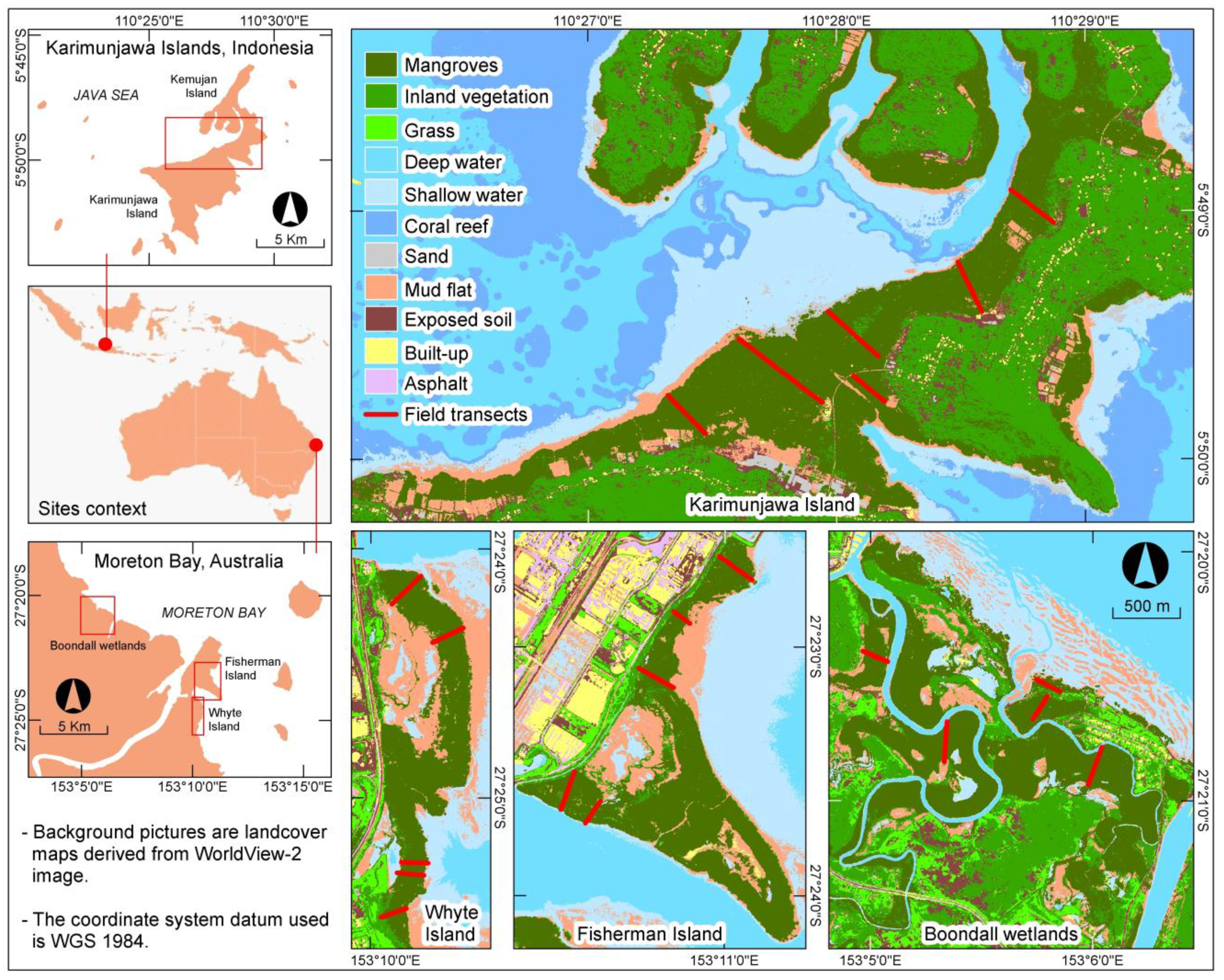
2.1. Study Area

The research was conducted in two mangrove areas; the mouth of the Brisbane River, northern Moreton Bay, Southeast Queensland, Australia and Karimunjawa National Park, Central Java, Indonesia (Figure 2). The first site (between 153°3ʹ41ʺ–153°11ʹ20ʺE and 27°19ʹ41ʺ–27°25ʹ31ʺS) is a sub-tropical lowland area including Whyte Island, Fisherman Island and Boondall wetlands, approximately 15 km northeast of Brisbane city. It is one of Australia’s premier wetlands and a Ramsar Convention listed wetland, with extensive stands of mangroves [38]. Avicennia marina is the dominant mangrove species, which comprises approximately 75% of the entire mangrove community within this region [39]. Other species, such as Rhizophora stylosa, Ceriops australis, Bruguiera gymnorhiza, Excoecaria agallocha, and Aegiceras corniculatum, are occasionally present [40]. The second site (between 110°24ʹ10ʺ–110°30ʹ10ʺE and 4°47ʹ48ʺ–5°50ʹ12ʺS) is located in the Java Sea with a tropical climate, approximately 125 km north of Semarang city. Mangroves in Karimunjawa National Park exist mainly in the fringing area on the western side of the two main islands, Karimunjawa and Kemujan. For simplicity we refer this site as Karimunjawa Island. According to a Karimunjawa National Park Office report [41], there are 45 mangrove species in this area (27 true mangroves and 18 mangrove associates), and Rhizophora stylosa is the dominant mangrove species. The Moreton Bay site was the primary site used to develop the methods and rule sets to map mangrove information at multiple levels and the Karimunjawa site was used to test the applicability of the method at a different mangrove location.

Figure 2. Study sites showing the major land-cover types and the field transects across the mangrove zonations.

Figure 2. Study sites showing the major land-cover types and the field transects across the mangrove zonations.

2.2. Image Datasets

This study used Landsat TM (TM), ALOS AVNIR-2 (AVNIR-2) and WorldView-2 (WV-2) multispectral images of the mouth of the Brisbane River and Karimunjawa Island to cover the variation of image spatial resolutions investigated, with the addition of LiDAR data and aerial photos for the Moreton Bay sites (Table 1). The WorldView-2 images were obtained at a high level of geometric correction (LV3X). The TM and AVNIR-2 images were geo-referenced based on the WV-2 image. The image pixel values (in digital numbers) were converted to top-of-atmosphere (TOA) spectral radiance using ENVI 4.8 (ITT Systems, ITT Exelis, Herndon, VA, USA). Further atmospheric correction was then performed to convert TOA spectral radiance to at surface reflectance using the Fast Line-of-sight Atmospheric Analysis of Hypercubes (FLAASH) atmospheric correction model for TM and WV-2 images, with the atmospheric visibility parameter estimated from the moderate-resolution imaging spectroradiometer (MODIS) aerosol product [42]. We applied a relative dark-pixel subtraction atmospheric correction method for AVNIR-2 images due to the lack of the satellite scanning position information. The Gram-Schmidt spectral sharpening image fusion technique [43] was applied to produce a pan-sharpened WorldView-2 image with a 0.5 m pixel size. This pan-sharpening technique was selected because it preserves the original spectral information of the image, and can be simultaneously applied to multispectral bands. A Canopy Height Model (CHM), Digital Terrain Model (DTM), and fractional canopy cover (FCC) were derived from the LiDAR data using lasheight, lasgrid, and lascanopy modules from LAStools (rapidlasso Gmbh., Germany). The CHM and DTM were used in combination with the multispectral images to define the boundary of mangroves and produce a mangrove structural composition map for the Moreton Bay site. Finally, a very high-spatial resolution aerial photograph (7.5 cm pixel size) with true color layers (www.nearmap.com) of Moreton Bay was used as a reference to analyze the classification accuracy of the produced maps.

Table 1. Image datasets used in this study.

Image Type	Moreton Bay Image Acquisition Date	Karimunjawa Island Image Acquisition Date	Pixel Size	Spectral Attributes (nm)	Geometric Attributes
Landsat TM	14 April 2011	31 July 2009	30 m	Blue (452–518), green (528–609), red (626–693), NIR (776–904), MIR1 (1567–1784), MIR2 (2097–2349)	Level 1T
ALOS AVNIR-2	10 April 2011	19 February 2009	10 m	Blue (420–500), green (520–600), red (610–690), NIR (760–890)	Level 1B2G
WorldView-2	14 April 2011	24 May 2012	2 m (multi), 0.5 m (pan)	Coastal blue (400–450), blue (450–510), green (510–580), yellow (585–625), red (630–690), red edge (705–745), NIR1 (770-895), NIR2 (860–1040), panchromatic (450–800)	Level 3X
LiDAR	April 2009	-	2.8 pts/m2	-	Geo-referenced
Aerial photo	14 January 2011	-	7.5 cm	RGB image	Geo-referenced

Table 1. Image datasets used in this study.

Image Type	Moreton Bay Image Acquisition Date	Karimunjawa Island Image Acquisition Date	Pixel Size	Spectral Attributes (nm)	Geometric Attributes
Landsat TM	14 April 2011	31 July 2009	30 m	Blue (452–518), green (528–609), red (626–693), NIR (776–904), MIR1 (1567–1784), MIR2 (2097–2349)	Level 1T
ALOS AVNIR-2	10 April 2011	19 February 2009	10 m	Blue (420–500), green (520–600), red (610–690), NIR (760–890)	Level 1B2G
WorldView-2	14 April 2011	24 May 2012	2 m (multi), 0.5 m (pan)	Coastal blue (400–450), blue (450–510), green (510–580), yellow (585–625), red (630–690), red edge (705–745), NIR1 (770-895), NIR2 (860–1040), panchromatic (450–800)	Level 3X
LiDAR	April 2009	-	2.8 pts/m2	-	Geo-referenced
Aerial photo	14 January 2011	-	7.5 cm	RGB image	Geo-referenced

2.3. Field Datasets

Fieldwork was conducted during April 2012 (for Moreton Bay sites) and July 2012 (for Karimunjawa Island) to collect information on vegetation structure and composition in the study areas. Twenty-one (200 to 300 m long) field transects were established perpendicular to the shoreline to record the variation of mangrove vegetation structure and species composition at different zones (Figure 2). These field transects were purposively selected to represent the variation of local mangrove zonation and at an accessible location. Plots of 10 m × 10 m consecutive quadrats were sampled along the transect lines to record mangrove biophysical properties in the field including canopy height, vegetation formation type, canopy cover, and dominant species. Positions of the start and the end of each sampling plot along the transect line were measured using a 12 channels Global Positioning System (GPS) receiver; using an average reading time for each point between 400 and 600 seconds (with a positional accuracy of 4–6 m) to maximize the GPS signal reception underneath the mangrove canopy. Additional control points identifiable both in the field and image were used to ensure the precise overlay of the transects and the image data. Canopy height was measured every 5 m along the transect using a TruPulse 360 laser rangefinder. Any canopy gaps found at the point of measurement were recorded, and the closest canopy was measured as additional data. The mangrove structural formation for each plot was determined using an Australian vegetation structural formation table [44]. Canopy cover was recorded using a digital camera at the center of four quarters of the plots (four 5 m quadrats), at a height of 1 m above ground and looking straight up. The photos were subsequently analyzed using CAN-EYE imaging software (http://www6.paca.inra.fr/can-eye) to determine the percentage of canopy cover. The dominant species within each 10 m x 10 m plot were identified using mangrove species identification books [40,45].

Four distinct mangrove zonations were identified from the high-spatial resolution images for both study sites and verified by field visits (Table 2). For Moreton Bay mangroves, Avicennia marina is the dominant mangrove species throughout each zonation, but different mangrove structural formation occurred within each zone. From the shoreline towards land, these zones represent mature closed forest, low-closed forest with single stems (some individual Rhizophora stylosa or Ceriops tagal were found in this zone), low-closed forest with single/multi stems, and open scrub. For Karimunjawa Islands, the dominant mangrove structural formation is closed forest, with more variety of mangrove species throughout the zonations. Tall trees of Rhizophora apiculata dominate the fringing shoreline area, followed by zones of highly-mixed Bruguiera gymnorhiza, Bruguiera cylindrical, Xylocarpus granatum and Excoecaria agallocha. The third and fourth zonations were mixes of Ceriops tagal and Lumnitzera racemosa with different vegetation structural formation.

Table 2. Mangrove canopy height, formation type, canopy cover and dominant species derived from field data sampled across the vegetation zones at four study sites.

Mangrove Zones*	Whyte Island	Fisherman Island	Boondall Wetlands	Karimunjawa Islands
Zone 1	10–12 m, closed forest (M4) with single- or multi-stems, high-density canopy cover, Avicennia marina trees.	8–11 m, closed forest (M4) with single- or multi-stems, high-density canopy cover, Avicennia marina trees.	8–10.5 m, closed forest (M4) with single- or multi-stems, very high-density canopy cover, Avicennia marina trees with some patches of Ceriops tagal.	11–15 m, closed forest (M4) with single- or multi-stems, very high-density canopy cover, Rhizophora apiculata trees with some individual Bruguiera gymnorhiza.
Zone 2	6–8 m, low-closed forest (I4) with single-stem, very high-density canopy cover, Avicennia marina trees with some individual Rhizophora stylosa.	8–10 m, low-closed forest (I4) with single-stem, high-density canopy cover, Avicennia marina with some individual Rhizophora stylosa and patches of Ceriops tagal.	7–9 m, low-closed forest (I4) with single-stem, very high-density canopy cover, Avicennia marina with some individual Rhizophora stylosa.	10–13 m, closed forest (M4) with single-stems, very high-density canopy cover, Bruguiera gymnorhiza, Bruguiera cylindrical, Xylocarpus granatum and Excoecaria agallocha.
Zone 3	4–7 m, low-closed forest (I4) with single- or multi-stems, medium-density canopy cover, Avicennia marina.	4–9 m, low-closed forest (I4) with single-stem, high-density canopy cover, Avicennia marina.	5–7.5 m, low-closed forest (I4) with single-stem, very high-density canopy cover, Avicennia marina.	7–10 m, low-closed forest (I4) with single- or multi-stems, high-density canopy cover, Ceriops tagal and Lumnitzera racemosa.
Zone 4	1–3 m, open scrub (S3) with multi-stems, low-density canopy cover, Avicennia marina.	2.5–4 m, open scrub (S3) with single- or multi-stems, low-density canopy cover, Avicennia marina.	1.5–5 m, open scrub (S3) with single- or multi-stems, medium-density canopy cover, Avicennia marina.	4–9 m, low multi-stem forest (VL4) with multi-stems, medium-density canopy cover, Ceriops tagal and Lumnitzera racemosa.

Note: Zone 1, 2, 3, and 4 for the Moreton Bay sites are centered at about 25, 75, 125, and 175 m, respectively, from the coastline; and 25, 150, 250, and 350 m from the coastline for the Karimunjawa site.

Table 2. Mangrove canopy height, formation type, canopy cover and dominant species derived from field data sampled across the vegetation zones at four study sites.

Mangrove Zones*	Whyte Island	Fisherman Island	Boondall Wetlands	Karimunjawa Islands
Zone 1	10–12 m, closed forest (M4) with single- or multi-stems, high-density canopy cover, Avicennia marina trees.	8–11 m, closed forest (M4) with single- or multi-stems, high-density canopy cover, Avicennia marina trees.	8–10.5 m, closed forest (M4) with single- or multi-stems, very high-density canopy cover, Avicennia marina trees with some patches of Ceriops tagal.	11–15 m, closed forest (M4) with single- or multi-stems, very high-density canopy cover, Rhizophora apiculata trees with some individual Bruguiera gymnorhiza.
Zone 2	6–8 m, low-closed forest (I4) with single-stem, very high-density canopy cover, Avicennia marina trees with some individual Rhizophora stylosa.	8–10 m, low-closed forest (I4) with single-stem, high-density canopy cover, Avicennia marina with some individual Rhizophora stylosa and patches of Ceriops tagal.	7–9 m, low-closed forest (I4) with single-stem, very high-density canopy cover, Avicennia marina with some individual Rhizophora stylosa.	10–13 m, closed forest (M4) with single-stems, very high-density canopy cover, Bruguiera gymnorhiza, Bruguiera cylindrical, Xylocarpus granatum and Excoecaria agallocha.
Zone 3	4–7 m, low-closed forest (I4) with single- or multi-stems, medium-density canopy cover, Avicennia marina.	4–9 m, low-closed forest (I4) with single-stem, high-density canopy cover, Avicennia marina.	5–7.5 m, low-closed forest (I4) with single-stem, very high-density canopy cover, Avicennia marina.	7–10 m, low-closed forest (I4) with single- or multi-stems, high-density canopy cover, Ceriops tagal and Lumnitzera racemosa.
Zone 4	1–3 m, open scrub (S3) with multi-stems, low-density canopy cover, Avicennia marina.	2.5–4 m, open scrub (S3) with single- or multi-stems, low-density canopy cover, Avicennia marina.	1.5–5 m, open scrub (S3) with single- or multi-stems, medium-density canopy cover, Avicennia marina.	4–9 m, low multi-stem forest (VL4) with multi-stems, medium-density canopy cover, Ceriops tagal and Lumnitzera racemosa.

Note: Zone 1, 2, 3, and 4 for the Moreton Bay sites are centered at about 25, 75, 125, and 175 m, respectively, from the coastline; and 25, 150, 250, and 350 m from the coastline for the Karimunjawa site.

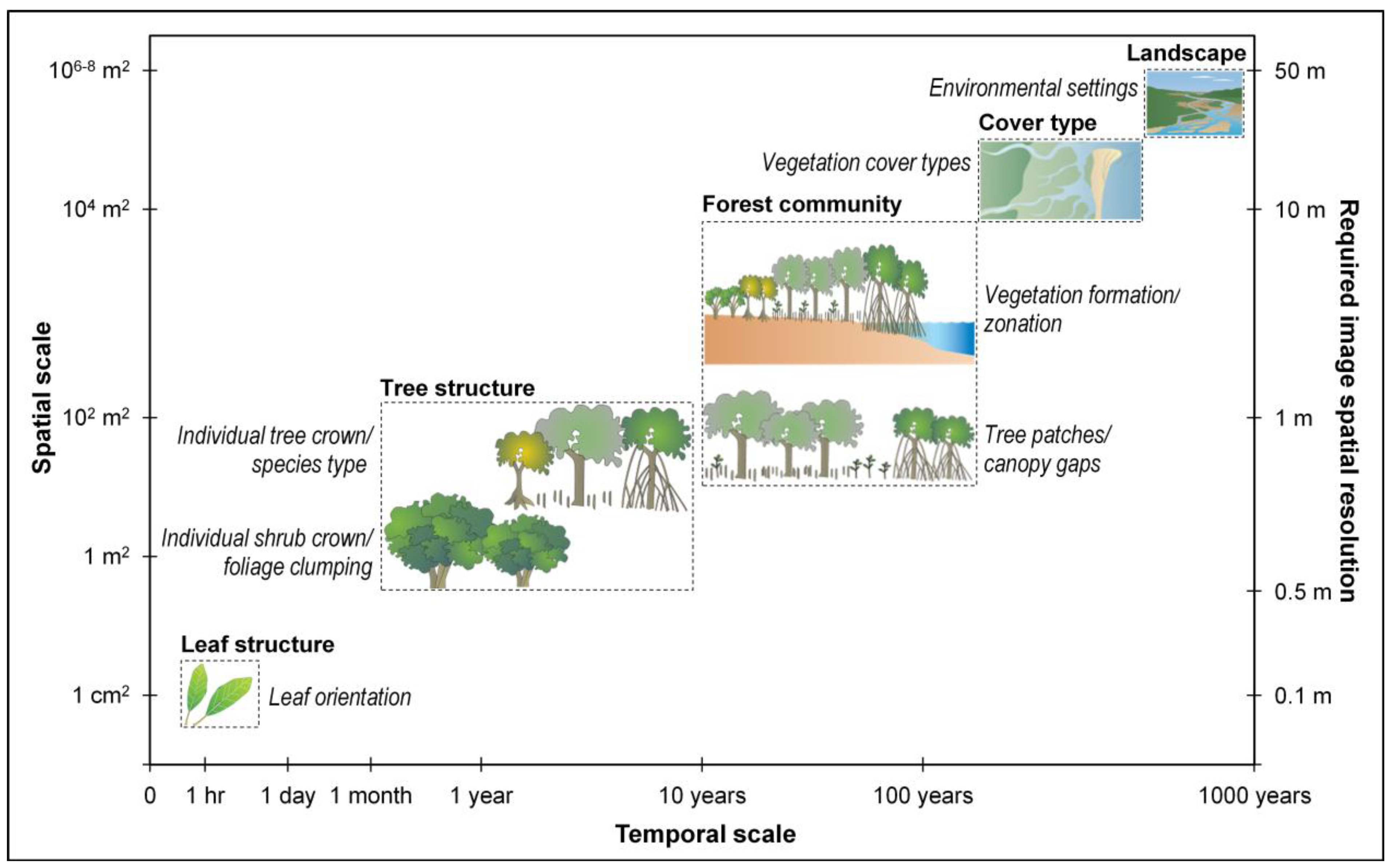
2.4. Mangrove Vegetation Structure Characterization

Prior to the mapping process, it is essential to perform an exploratory analysis to understand the spatial variability of the vegetation structure at different targeted locations and environment settings. This approach identifies the expected levels of detail able to be obtained from each site. We used semi-variograms to analyze the spatial structure of mangroves at the Moreton Bay and Karimunjawa Island sites. Semi-variograms are used for measuring the degree of dissimilarity between observations as a function of distance [46], and a review of its application in remote sensing was provided by Curran and Atkinson [47]. As demonstrated by Cohen [48], Johansen and Phinn [49], and Kamal et al. [30], the semi-variogram can be used to explore and describe the spatial variation of objects of interest in the image data in various forest environments. The equation for semi-variance γ(h) is:

$$\text{γ}(h) = \frac{1}{2n}{{\displaystyle \sum }}^{\text{}}{\left\{DN\left(x\right)-DN\left(x+h\right)\right\}}^2$$

(1)

where γ(h) represents half of the mathematical expectation of the squared differences of pixel pair values at a distance h. For image spectral data, γ(h) estimates the variability of pixel digital numbers (DN), as a function of spatial separation. The semi-variograms in this paper were derived from 21-line transects positioned across the mangrove zonations on the WV-2 image, coinciding with the field transects. We used all bands of the WV-2 pan-sharpened data to produce semi-variograms, but only the green band is presented because it depicts the highest detailed level of mangrove vegetation information compared to the other bands [30].

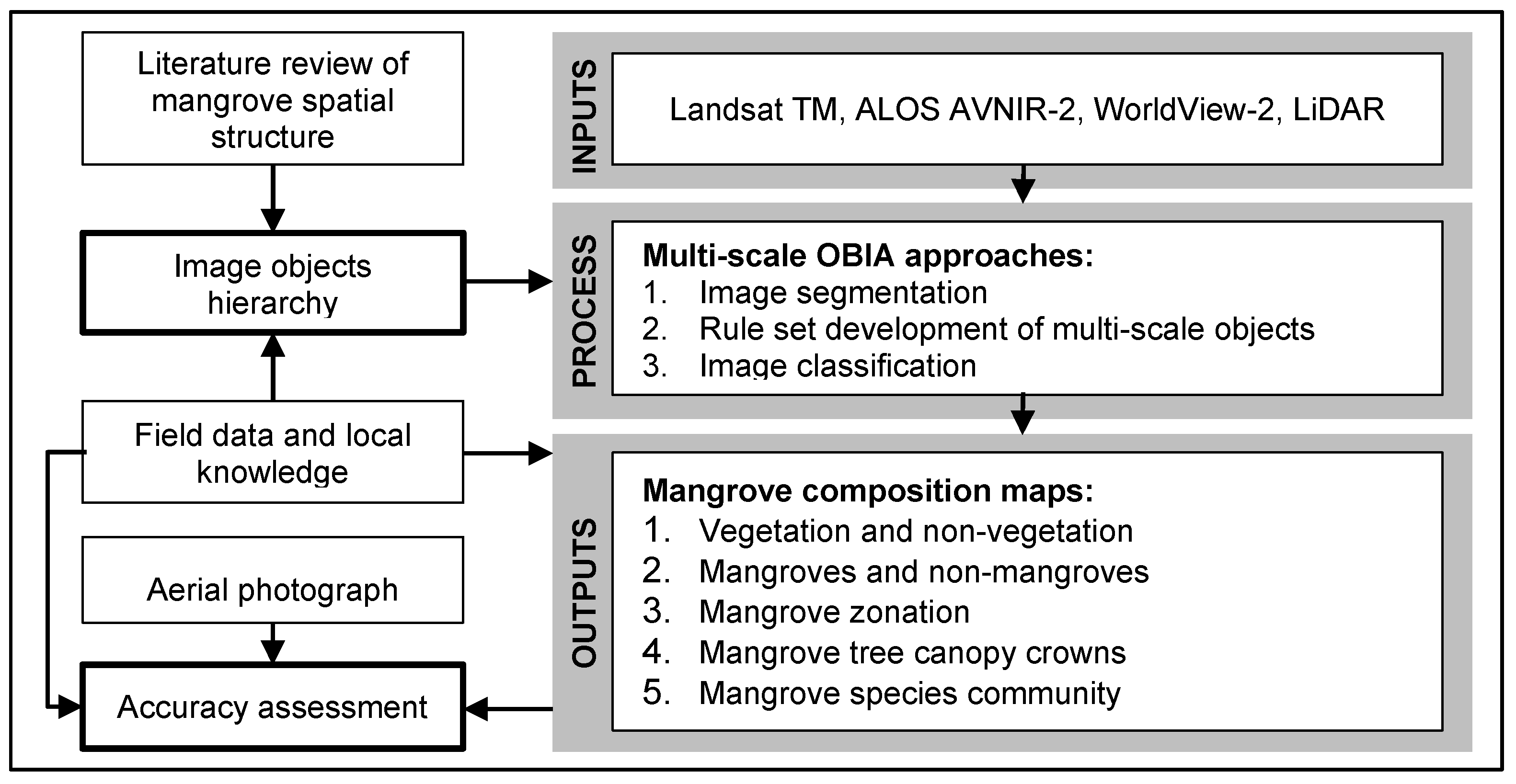
2.5. Overview of the GEOBIA Approach

The GEOBIA mapping process started with developing a conceptual hierarchical structure of mangrove objects based on literature on mangrove spatial structure and the analysis described in Section 2.4, fieldwork data, and local knowledge (Figure 3). It shows the organization of mangrove features at various spatial scales and represents the objects of interest to be mapped. Inclusion of specific scales of mapped features is one of the main advantages of GEOBIA, which does this in a multi-scale hierarchical network of image objects derived through image segmentation [50,51]. Based on the conceptual hierarchy, five levels of mangrove features were selected (see output section in Figure 3). To perform the multi-scale mangrove mapping, eCognition Developer 8.7 [52] was exploited to develop the rule set and for executing the object-based routine.

Figure 3. Flowchart of the mapping process applied in this study.

Figure 3. Flowchart of the mapping process applied in this study.

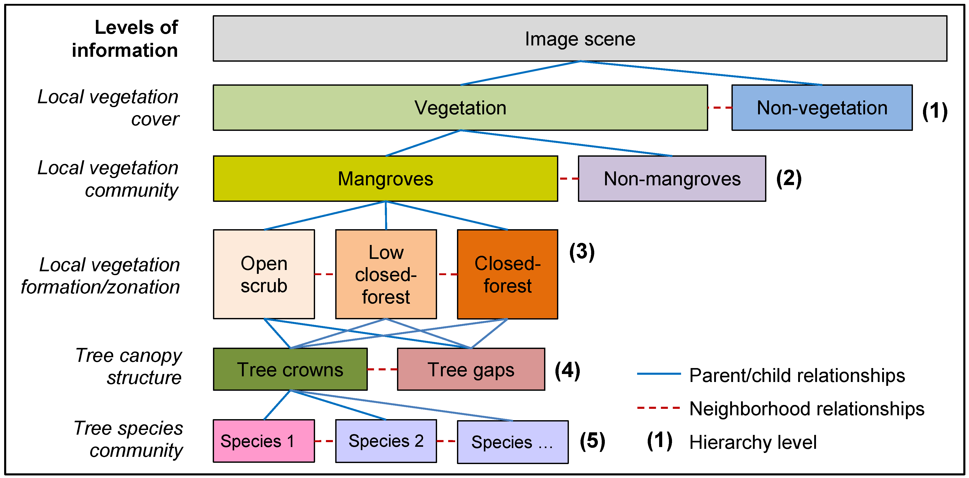
2.5.1. Classification Hierarchy and Rule Sets Development

Developing conceptual hierarchical levels of the objects of interests is essential in multi-scale mapping using GEOBIA [24,26,53]. This hierarchy shows the spatial organization of the objects in the landscape or image scene from a larger landscape unit into the smaller objects or component units. We used the landscape scaling ladder concept [24,26,54] to break down the complexity of targeted mangrove information into manageable units that still linked across scales (Figure 4). In the hierarchy, the “super-level” objects act as containers for its “sub-levels”, and work within parent and child relationship; while objects at the same level have a neighborhood relationship [26,52]. There are several advantages of having this hierarchy in place, as it provides a logical sequential mapping process, has a clear multi-scale context of the targeted objects and their relationships, and provides control over the process within a certain level and object container.

From the object hierarchy we developed a strategy and procedure to identify and map the targeted objects individually, which was documented in the form of rule sets. For example, conceptually mangroves can be found within vegetation features in the image, and it also serves as the container of several lower hierarchical levels such as mangrove zonations, tree crown and canopy gaps, and individual tree species. At this stage, it is also necessary to identify some potential properties commonly embedded in these features in the image, which could be spectral, textural, and/or contextual (i.e., the relative position of the targeted object in relation to other objects that provides useful information for classifying the targeted object, such as distance, adjacency, location, and association [25]) information of the targeted features. Together, the conceptual object hierarchy and mapping strategy provide a feasible scenario to apply in the rule set processes to address the predefined research problem. Table 3 shows the documented multi-scale mapping scenario, membership rules and the classification processes developed for the Moreton Bay mangrove site. Exploratory work was done to find the best image band algorithm and associated threshold for each image and this is explained in more details in the corresponding sections. We do not provide the detailed rule set for Karimunjawa Island due to the limitation of paper space. However, it is available upon request, and the results comparison is discussed in Section 3.5.

Figure 4. Image objects hierarchy for multi-scale mangrove mapping, objects relationships, and the levels of information at each hierarchy level.

Figure 4. Image objects hierarchy for multi-scale mangrove mapping, objects relationships, and the levels of information at each hierarchy level.

Table 3. Summary of the membership rules used in the multi-scale mangrove classification rule sets for Moreton Bay mangroves. The numbers in the table correspond to section numbers in the method section of this paper.

No.	Information		Landsat TM	ALOS AVNIR-2	WorldView-2	WorldView-2 and LiDAR
2.5.2	Vegetation		Layer arithmetic	Layer arithmetic	Layer arithmetic	Layer arithmetic
			Multi-threshold seg.	Multi-threshold seg.	Multi-threshold seg.	Multi-threshold seg.
			FDI > 100	FDI > 200	FDI > 0	FDI > 0
	Non-vegetation		Not “Vegetation”	Not “Vegetation”	Not “Vegetation”	Not “Vegetation”
2.5.3	Mangroves		Within “Vegetation”	Within “Vegetation”	Within “Vegetation”	Within “Vegetation”
			Chessboard seg: 1	Chessboard seg: 1	Chessboard seg: 1	Chessboard seg: 1
			Mean 4 = 1500 − 3500	Mean 3 = 300 − 550	(7 − 5)/(3 − 5) = 8 − 22	(7 − 5)/(3 − 5) = 8 − 22
			Mean 5 = 900 − 1450	Mean 4 = 1000 − 3000	Mean 5 < 720	Mean 5 < 720
						Mean DTM < 1.5
	Non-mangroves		Not “Mangroves”	Not “Mangroves”	Not “Mangroves”	Not “Mangroves”
2.5.4	Zonation bands			Within “Mangroves”	Within “Mangroves”	Within “Mangroves”
				Multiresolution seg. (SP:10, s:0.1, c:0.5)	Multiresolution seg. (SP:25, s:0.1, c:0.5)	Multiresolution seg. (SP:25, s:0.1, c:0.5)
		Zone 1	-	1.5 < 4/(3+1) < 4	0 > 7/(5+6) < 1.36	Mean CHM > 10
				Coast dist < 75m	Coast dist < 75m	FCC < 1
		Zone 2	-	2.5 < 4/(3+1) < 6	7/(5+6) > 0	7 < CHM < 10
				25>Coast dist<100m	25>Coast dist<100m	0.95 > FCC <1
		Zone 3	-	1.5 < 4/(3+1) < 4	0 > 7/(5+6) < 1.36	3 < CHM < 7
				Coast dist > 100m	Coast dist > 100m	FCC < 0.98
						Coast dist > 75
		Zone 4	-	1.5 < 4/(3+1) < 6	7/(5+6) > 1.36	CHM < 3
				Coast dist > 100m	Coast dist > 100m	FCC < 0.98
2.5.5	Tree canopy	Canopy gaps	-	-	Within “Mangroves”	Within “Mangroves”
					Chessboard seg: 1 Within “Mangroves”	Chessboard seg: 1 Mean CHM < 3
					Mean PC1 > 500
					Mean PC2 < -250
		Tree crowns	-	-	Not “Canopy gaps”	Not “Canopy gaps”
					Seed based on local maxima of NIR1.	Seed based on local maxima of CHM.
					Grow seed by ratio to neighbor < 1.2.	Grow seed by ratio to neighbor < 1.5.
					Opening the seed.	Opening the seed.
2.5.6	Individual species		-	-	Within “Tree crowns”.
					Nearest Neighbor classification with samples taken from the individual tree crown.

FDI: Forest Discrimination Index, NIR: near-infrared, MIR: mid-infrared, DTM: digital terrain model, CHM: canopy height model, FCC: fractional canopy cover, PC: principal component, SP: scale parameter, s: shape, c: compactness, italic numbers represent band order for the associated images, the conditional operator used on each membership rule was “and (min)”.

Table 3. Summary of the membership rules used in the multi-scale mangrove classification rule sets for Moreton Bay mangroves. The numbers in the table correspond to section numbers in the method section of this paper.

No.	Information		Landsat TM	ALOS AVNIR-2	WorldView-2	WorldView-2 and LiDAR
2.5.2	Vegetation		Layer arithmetic	Layer arithmetic	Layer arithmetic	Layer arithmetic
			Multi-threshold seg.	Multi-threshold seg.	Multi-threshold seg.	Multi-threshold seg.
			FDI > 100	FDI > 200	FDI > 0	FDI > 0
	Non-vegetation		Not “Vegetation”	Not “Vegetation”	Not “Vegetation”	Not “Vegetation”
2.5.3	Mangroves		Within “Vegetation”	Within “Vegetation”	Within “Vegetation”	Within “Vegetation”
			Chessboard seg: 1	Chessboard seg: 1	Chessboard seg: 1	Chessboard seg: 1
			Mean 4 = 1500 − 3500	Mean 3 = 300 − 550	(7 − 5)/(3 − 5) = 8 − 22	(7 − 5)/(3 − 5) = 8 − 22
			Mean 5 = 900 − 1450	Mean 4 = 1000 − 3000	Mean 5 < 720	Mean 5 < 720
						Mean DTM < 1.5
	Non-mangroves		Not “Mangroves”	Not “Mangroves”	Not “Mangroves”	Not “Mangroves”
2.5.4	Zonation bands			Within “Mangroves”	Within “Mangroves”	Within “Mangroves”
				Multiresolution seg. (SP:10, s:0.1, c:0.5)	Multiresolution seg. (SP:25, s:0.1, c:0.5)	Multiresolution seg. (SP:25, s:0.1, c:0.5)
		Zone 1	-	1.5 < 4/(3+1) < 4	0 > 7/(5+6) < 1.36	Mean CHM > 10
				Coast dist < 75m	Coast dist < 75m	FCC < 1
		Zone 2	-	2.5 < 4/(3+1) < 6	7/(5+6) > 0	7 < CHM < 10
				25>Coast dist<100m	25>Coast dist<100m	0.95 > FCC <1
		Zone 3	-	1.5 < 4/(3+1) < 4	0 > 7/(5+6) < 1.36	3 < CHM < 7
				Coast dist > 100m	Coast dist > 100m	FCC < 0.98
						Coast dist > 75
		Zone 4	-	1.5 < 4/(3+1) < 6	7/(5+6) > 1.36	CHM < 3
				Coast dist > 100m	Coast dist > 100m	FCC < 0.98
2.5.5	Tree canopy	Canopy gaps	-	-	Within “Mangroves”	Within “Mangroves”
					Chessboard seg: 1 Within “Mangroves”	Chessboard seg: 1 Mean CHM < 3
					Mean PC1 > 500
					Mean PC2 < -250
		Tree crowns	-	-	Not “Canopy gaps”	Not “Canopy gaps”
					Seed based on local maxima of NIR1.	Seed based on local maxima of CHM.
					Grow seed by ratio to neighbor < 1.2.	Grow seed by ratio to neighbor < 1.5.
					Opening the seed.	Opening the seed.
2.5.6	Individual species		-	-	Within “Tree crowns”.
					Nearest Neighbor classification with samples taken from the individual tree crown.

FDI: Forest Discrimination Index, NIR: near-infrared, MIR: mid-infrared, DTM: digital terrain model, CHM: canopy height model, FCC: fractional canopy cover, PC: principal component, SP: scale parameter, s: shape, c: compactness, italic numbers represent band order for the associated images, the conditional operator used on each membership rule was “and (min)”.

2.5.2. Vegetation and Non-Vegetation Separation

The first classification level in the multi-scale mapping process generated a mask to separate vegetation and non-vegetation features (i.e., water bodies, soils, and other artificial surfaces) in the image. In this study, we modified the Forest Discrimination Index (FDI) developed by Bunting and Lucas [55] to separate vegetation and non-vegetation as follow:

$$\mathrm{F}\mathrm{D}\mathrm{I} = \mathrm{N}\mathrm{I}\mathrm{R} - (\mathrm{R}\mathrm{e}\mathrm{d} + \mathrm{G}\mathrm{r}\mathrm{e}\mathrm{e}\mathrm{n})$$

(2)

This equation was derived by examining the spectral reflectance pattern of targeted features from the WV-2 image bands that had the greatest spectral separation between vegetation and non-vegetation features, as indicated by the standard deviation bars in Figure 5. The near infra-red1 (NIR1) band, as expected, provided consistently high spectral response of all types of healthy vegetation and gave the greatest spectral separation between features (Figure 5). Water and artificial surfaces (building roofs and asphalt) had high spectral reflectance in the green band (band 3) and lower spectral reflectance in the red band (band 5), but greater separation from vegetation features. In this case, the sum of the green and red bands could be greater, lower or equal to the value of the near infrared1 band. Therefore, for the WV-2 image, FDI values greater than zero represent all types of vegetation features, and zero or negative values represent non-vegetation features (Figure 6b). Different threshold values were applied to other images due to variation of object spectral reflectance responses between images (Table 3). We used layer arithmetic and multi-threshold segmentation algorithms to implement this process in the eCognition Developer 8.7 software, and creating a discrete delineation between vegetation and non-vegetation based on image pixel values.

Figure 5. Spectral reflectance profiles of the major land cover types extracted from WV-2 image within the Moreton Bay site.

Figure 5. Spectral reflectance profiles of the major land cover types extracted from WV-2 image within the Moreton Bay site.

2.5.3. Mangroves and Non-Mangroves Discrimination

Mangroves and non-mangroves within the vegetation class were separated by combining thresholds of image bands or band algorithms that were sensitive to mangrove features. Chessboard segmentation was applied to preserve the pixel value of the image. For spectral recognition of mangroves, the near-infrared reflectance spectrum revealed different reflectance levels related to the internal leaf structure and facilitated mangrove discrimination from other objects [14]. It is also evident from the spectral reflectance profile in Figure 5 that mangroves has a distinguishable spectral profile from other vegetation objects; specifically in the green, red, and NIR bands of the WV-2 image where the spectral separation are optimal.

Figure 6. Subset of Whyte Island maps, showing (a) WV-2 standard false color composite, (b) vegetation (V) and non-vegetation (NV) discrimination using FDI, (c) spectral-based mangroves (M) and non-mangroves (NM) separation, and (d) band combination image to enhance the mangrove zonations. Tree crown delineation process showing (e) color composite of PC1, PC2, PC1 (RGB), (f) masked canopy gaps (white), (g) tree canopy seeds (red) on top of NIR band, and (h) tree crown polygons derived from region growing.

Figure 6. Subset of Whyte Island maps, showing (a) WV-2 standard false color composite, (b) vegetation (V) and non-vegetation (NV) discrimination using FDI, (c) spectral-based mangroves (M) and non-mangroves (NM) separation, and (d) band combination image to enhance the mangrove zonations. Tree crown delineation process showing (e) color composite of PC1, PC2, PC1 (RGB), (f) masked canopy gaps (white), (g) tree canopy seeds (red) on top of NIR band, and (h) tree crown polygons derived from region growing.

At the Moreton Bay site, a ratio of the spectral reflectance distance between NIR to red, and green to red ([NIR-red]/[green-red]) was found to be effective in separating mangrove from non-mangrove objects in the WV-2 imagery (Figure 6c). The NIR and red bands were also found useful for discriminating mangrove objects in the AVNIR-2 imagery, as were the NIR and the first mid infrared (MIR1) band for the TM image (Table 3). To enable comparison with the spectral-based only approach, the contextual information in the form of a DTM derived from LiDAR data was also used in this process in combination with the WV-2 image. The DTM was used to set an elevation boundary above sea level for mangrove habitats that commonly occur in the lower parts of tidal flats in coastal or riverine areas, which is frequently inundated by saline water. Limiting the delineation to the typical elevation of mangrove habitats will increase the accuracy of the classification and compensate for limitations of spectral-based recognition.

2.5.4. Mangrove Zonation Pattern Delineation

Mangrove zonation boundaries at the study sites follow the topographic contours which are possibly indicative of tidal inundation levels [22]. From the field survey, it was established that these zonations represent a variation of canopy cover density, stem structure, dominant species, and tree height (Table 2). Optical remote sensing data can often distinguish different mangrove zones based on the spectral reflectance of dominant mangrove species within each zone [56]. Multi-resolution segmentations with the scale parameters of 10 and 25 were applied to the AVNIR-2 and WV-2 image data, respectively, within the mangrove class to aggregate the zonation pattern. Using the AVNIR-2 and WV-2 images, a combination of band ratios and the distance from the coastline (Table 3) facilitated the differentiation of mangrove zonation boundaries (Figure 6d). Exploratory work was carried out to find the best image band ratio and associated threshold for each image to enhance the difference between each zonation. However, due to the large pixel size and the narrow mangrove zonation bands, TM was unable to differentiate the zonation pattern. As a comparison, we also incorporated the CHM and fractional canopy cover (FCC) derived from LiDAR data to differentiate the mangrove zonations based on tree height and canopy cover density.

2.5.5. Mangrove Tree Crown and Gap Delineation

To delineate individual mangrove tree crowns and gaps we modified the “valley following” [57] and “region growing” [58] approaches, and applied these in the eCognition Developer software. The basic principle of tree crown delineation is well-described using three-dimensional “radiometric topography” analogy of tree crowns [58]. The valleys (local minima) which have lower spectral reflectance (i.e., in the NIR or panchromatic band) represent the boundary of tree crowns, while the peaks, which have local maxima, are treated as seeds and will be grown towards the boundary of the valleys. The polygons created from this region-growing approach are the tree crowns. There are two implicit assumptions in these approaches; (1) the tree crown should be visually recognizable as a discrete object on the image (i.e., the pixel size of the image must be smaller than the average size of the tree), and (2) the tree crown is brighter (or has a higher pixel value) than the edge of the crown [59]. Therefore, we used the pan-sharpened WV-2 image with a pixel size of 50 cm to delineate the tree crowns. Chessboard segmentation with the value of 1 was applied to the mangrove class based on the pan-sharpened WV-2 image to obtain pixel level information for use in this process.

There were three main steps to delineate mangrove tree crowns. The first step was to find tree canopy gaps between trees as the boundary of the tree crowns. It is common in mangrove forest to have irregular stands and canopies with groups of trees often clumped into a single wider canopy, making the delineation of canopy gaps through shadow (local minima) growing difficult. Therefore, we used PC1 and PC2 of the image, which accounted for 99.84% of the variance to emphasize the different appearance between soil backgrounds or canopy gaps and mangrove tree canopies (Figure 6e,f). The second step was to find the tree top (local maxima) from the original NIR1 band and treat them as crown seeds (Figure 6g), and then grow it toward the canopy gaps border. We used a ratio of NIR1 spectral values of the adjacent pixels to the crown seed to grow the crown region in a looped iteration until the crown seed polygons reached the canopy gaps border. This rule set was developed to adapt the sample sites’ mangrove pattern, where there are noticeable canopy gaps between tree canopies. Modifications might be needed to apply this rule set to mangrove forests with limited canopy gaps. Finally the delineated tree crowns were refined using a pixel-based morphological opening operation to smooth the edge of the tree crown polygons (Figure 6h). As a comparison, we used the LiDAR data to delineate tree crowns based on the patterns of canopy height derived from the CHM.

2.5.6. Mangrove Species Community Identification

Delineated tree crowns were classified into main mangrove species found at the study sites using the pan-sharpened WV-2 multi-spectral image bands using a supervised nearest neighbor (NN) classifier. The extra textural information in the pan-sharpened imagery is important to include due to different vegetation structural characteristics of mangrove species. The boundary of tree species communities is also more apparent with smaller pixels. We applied an approach similar to the one developed by Gougeon and Lackie [60], where representative sample objects of each mangrove species were collected individually from the tree crown polygons, and used to generate signatures for each class. The nearest neighbor (NN) algorithm looks for the closest sample object in the feature space for each image object [52]. We used a standard NN algorithm based on the mean value of red, green, blue, PC2 layers, and the standard deviation of layer NIR1, with the selection of the object samples guided by the field species identification. However, due to the domination of Avicennia marina stands in Moreton Bay mangroves, it is difficult to identify the other species using this approach. Therefore, we applied this classifier to discriminate different communities of Avicennia marina in Moreton Bay mangroves.

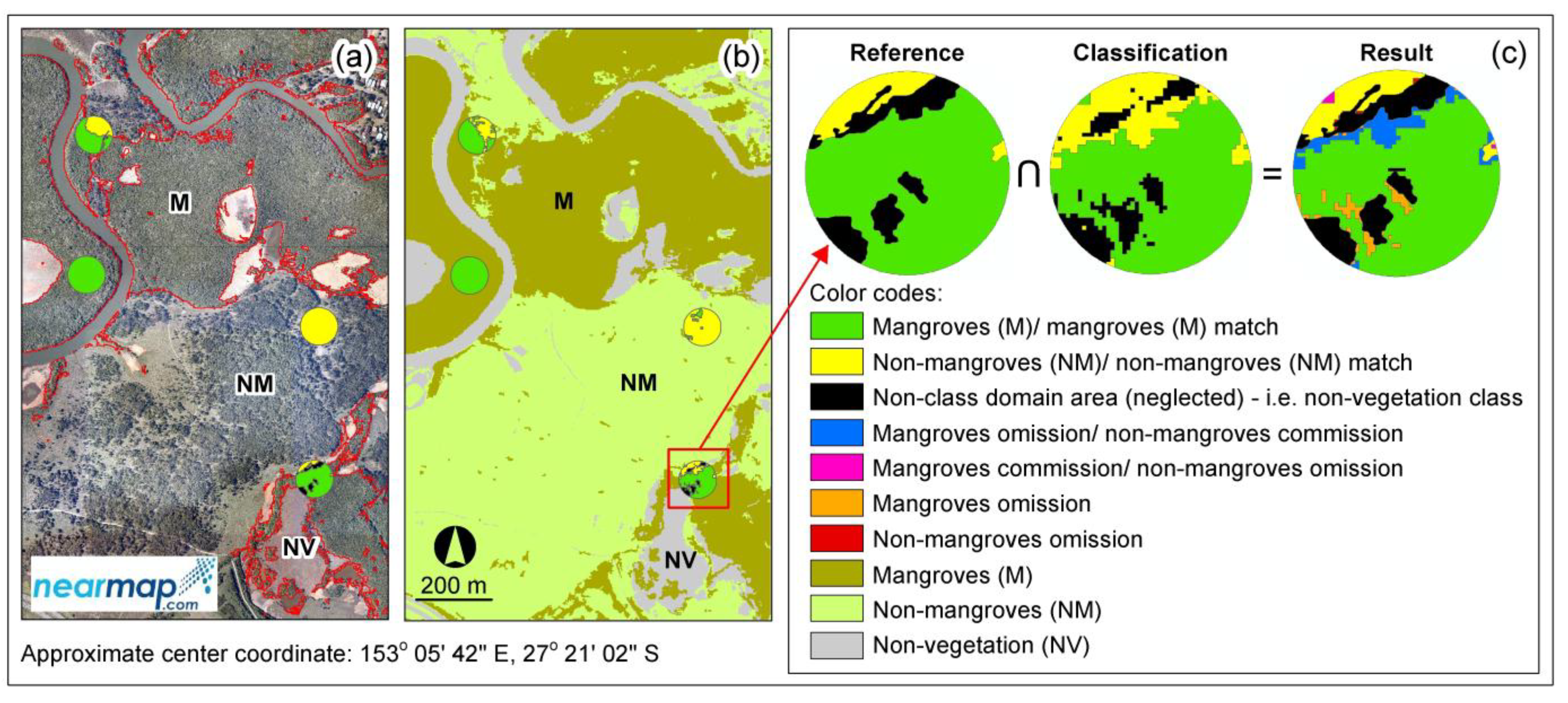
2.6. Mangrove Composition Mapping Validation

The accuracy assessment of GEOBIA requires assessment of the geometric accuracy (shape, symmetry and location) of the created image objects [61], because the geometry of image objects is an inherent property resulting from image segmentation. However, only limited number of published works describes the area-based accuracy approach developed for GEOBIA [35]. Among the significant results in this field were studies done by Zhan et al. [62] and Whiteside et al. [63] who developed a framework for assessing the quality of geometric properties of image objects based on the error matrix idea. An area-based accuracy assessment (Table 4) was used to measure the degree of similarity between the results of the classification and reference data from different aspects, including overall quality, user’s accuracy, and producer’s accuracy [62]. In addition, we also calculated the overall accuracy measure, which is defined as the ratio between the correctly classified area and the total area of observation. To perform this calculation, the reference data used in this measurement should have an area dimension matching the classified objects [62,63].

The accuracy assessments were performed for map results of levels 1 to 4 (see Figure 4) against the thematic maps derived from manual interpretation of a very-high-spatial resolution aerial photograph (7.5 cm pixel size) of the Moreton Bay mangroves. All of these features can be accurately discriminated and delineated from this imagery. This approach was selected due to the lack of reference information for the study sites for the accuracy assessment. The image interpretation results from the very high-spatial resolution aerial photographs were accepted to be correct without any form of accuracy assessment [64]. However, we did not perform the accuracy assessment for Karimunjawa Island due to the lack of the reference maps and very-high resolution aerial imagery. Following the approach by Whiteside et al. [63], we used a circular buffer with a 50 m radius of 30 random point samples within the “class domain areas” to calculate the area-based accuracy assessment. The circular buffer was used for practical reasons to create the area samples, and the number of points and buffer radius were chosen with regard to the size of the objects on the map being accuracy assessed. The resulting circular polygons were used to clip both the classified image objects and visually-interpreted reference map for area comparisons (Figure 7). A similar approach was implemented for the accuracy assessments of levels 3, 4, and 5. However, for level 3 we only plotted 10 random points and used a buffer radius of 20 m within each zonation because of the smaller area of the object class being validated. Ten random points with a 10 m radius buffer was used for levels 4 and 5. However, at the mangrove species level, we used South East Queensland mangrove composition maps (1:25,000) produced by the Queensland Herbarium [65] as reference data. This map was produced from aerial photograph interpretation combined with extensive fieldwork, which shows the mangrove species communities and their description of the Moreton Bay area.

Table 4. Area-based accuracy assessment equations [62,63].

Measure	Equations	Equation Number
Overall Quality (OQ)	$(|C{{\displaystyle \cap }}^{\text{}}R|)/(|C{{\displaystyle \cap }}^{\text{}}R|+|C{{\displaystyle \cap }}^{\text{}}R|+|C{{\displaystyle \cap }}^{\text{}}R|)$	3
User’s Accuracy (UA)	$(|C{{\displaystyle \cap }}^{\text{}}R|)/(|C|)$	4
Producer’s Accuracy (PA)	$(|C{{\displaystyle \cap }}^{\text{}}R|)/(|R|)$	5
Overall Accuracy (OA)	$(|C{{\displaystyle \cap }}^{\text{}}R|)/(|C{{\displaystyle \cup }}^{\text{}}R|)$	6

C is the area of the classified object and R is the area of the reference object, C∩R is the area of intersection between C and R, C∩R is the area of R not covered by C, C∩R is the area of C that is not covered by R, and C∪R is the area covered by both objects.

Table 4. Area-based accuracy assessment equations [62,63].

Measure	Equations	Equation Number
Overall Quality (OQ)	$(|C{{\displaystyle \cap }}^{\text{}}R|)/(|C{{\displaystyle \cap }}^{\text{}}R|+|C{{\displaystyle \cap }}^{\text{}}R|+|C{{\displaystyle \cap }}^{\text{}}R|)$	3
User’s Accuracy (UA)	$(|C{{\displaystyle \cap }}^{\text{}}R|)/(|C|)$	4
Producer’s Accuracy (PA)	$(|C{{\displaystyle \cap }}^{\text{}}R|)/(|R|)$	5
Overall Accuracy (OA)	$(|C{{\displaystyle \cap }}^{\text{}}R|)/(|C{{\displaystyle \cup }}^{\text{}}R|)$	6

C is the area of the classified object and R is the area of the reference object, C∩R is the area of intersection between C and R, C∩R is the area of R not covered by C, C∩R is the area of C that is not covered by R, and C∪R is the area covered by both objects.

Figure 7. Example of mangroves and non-mangroves area-based accuracy assessment; (a) reference map, (b) classified map from WV-2 image, and (c) classes produced from area intersection process.

Figure 7. Example of mangroves and non-mangroves area-based accuracy assessment; (a) reference map, (b) classified map from WV-2 image, and (c) classes produced from area intersection process.

3. Results and Discussion

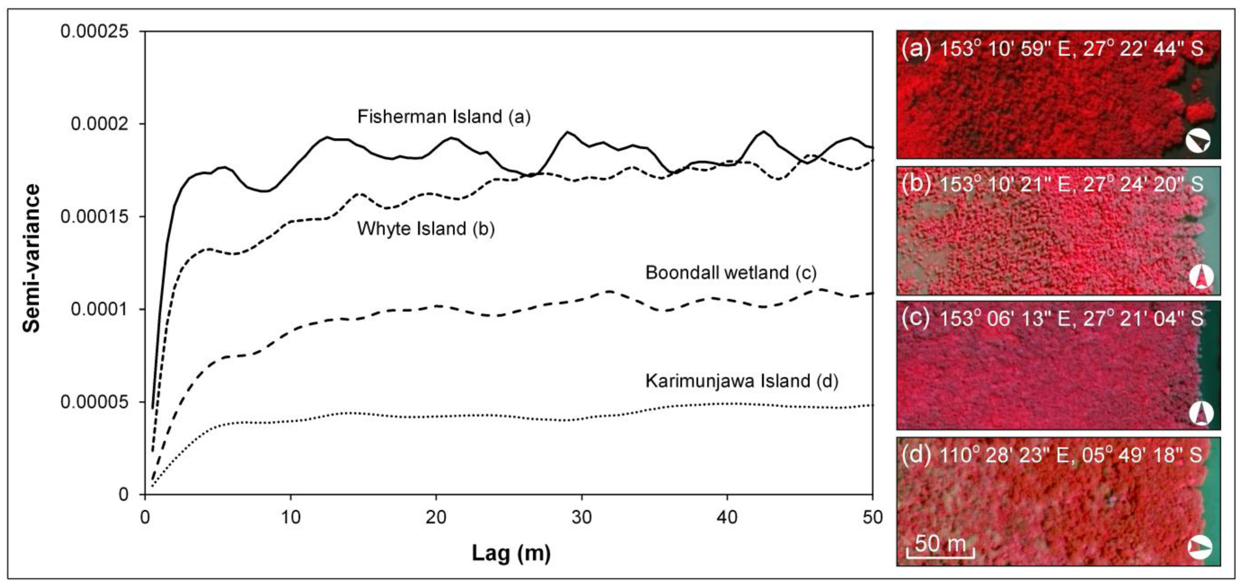
3.1. Mangrove Spatial Structure from Semi-Variogram Analysis

In this study, we were particularly interested in the forms of the semi-variograms, namely sill and periodicity. They are related to the density of objects and scene-scale level of variance [66,67], and provide an indication of a repetitive spatial pattern along the transect [67,68]. Figure 8 showed that Fisherman and Whyte Island mangroves have higher sill and periodicity than Boondall wetland and Karimunjawa Island mangroves. This pattern was attributed to the high variation in the degree of open-ness of mangrove canopy and the significant canopy gaps present in the Fisherman and Whyte Islands mangroves, allowing individual tree crowns to be detected. On the other hand, mangroves in the Boondall wetlands were dominated by low-closed Avicennia marina forest of homogeneous stems with very high-density canopy cover, and the mangroves in Karimunjawa Island mainly consisted of closed-mature mangrove trees with overlapping canopy crowns (Table 2). It was noticeable from the image (Figure 8c,d) that mangroves in Boondall wetlands and Karimunjawa Island have a smooth texture with minimum gaps between tree stands and some clumping of tree groups, preventing detection of individual tree crowns from the image. From the semi-variogram analysis, we hypothesized that mangroves on Fisherman and Whyte Islands have higher vegetation structural variability compared to the others, providing a higher level of information for mangrove mapping (i.e., up to the tree canopy crown level).

Figure 8. Subsets of green band semi-variograms, with up to 50 m lag distance, showing the variation of vegetation structure at different sites: (a) Fisherman Island, (b) Whyte Island, (c) Boondall wetlands and (d) Karimunjawa Island. Coordinates represent the approximate center of each image.

Figure 8. Subsets of green band semi-variograms, with up to 50 m lag distance, showing the variation of vegetation structure at different sites: (a) Fisherman Island, (b) Whyte Island, (c) Boondall wetlands and (d) Karimunjawa Island. Coordinates represent the approximate center of each image.

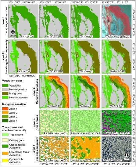
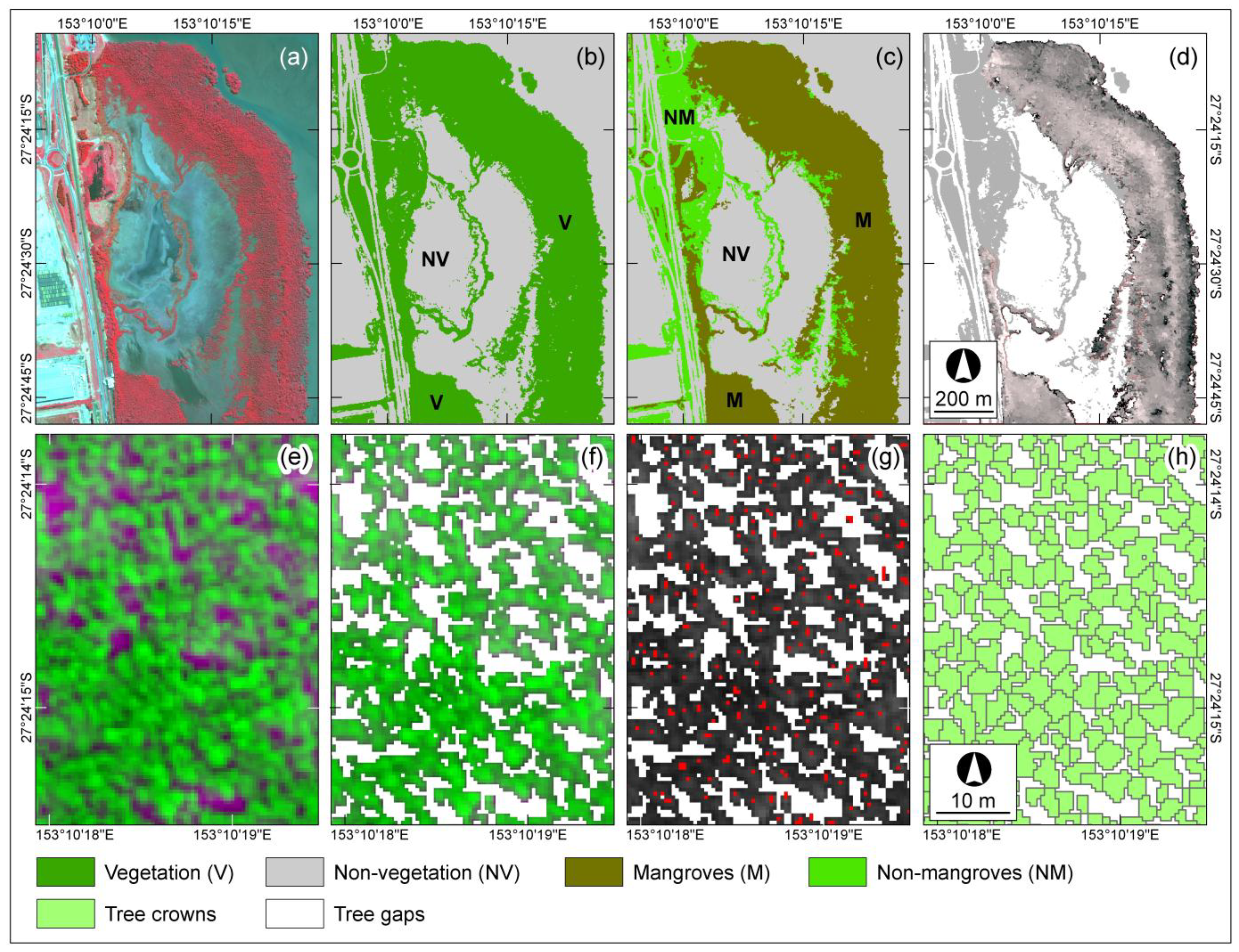
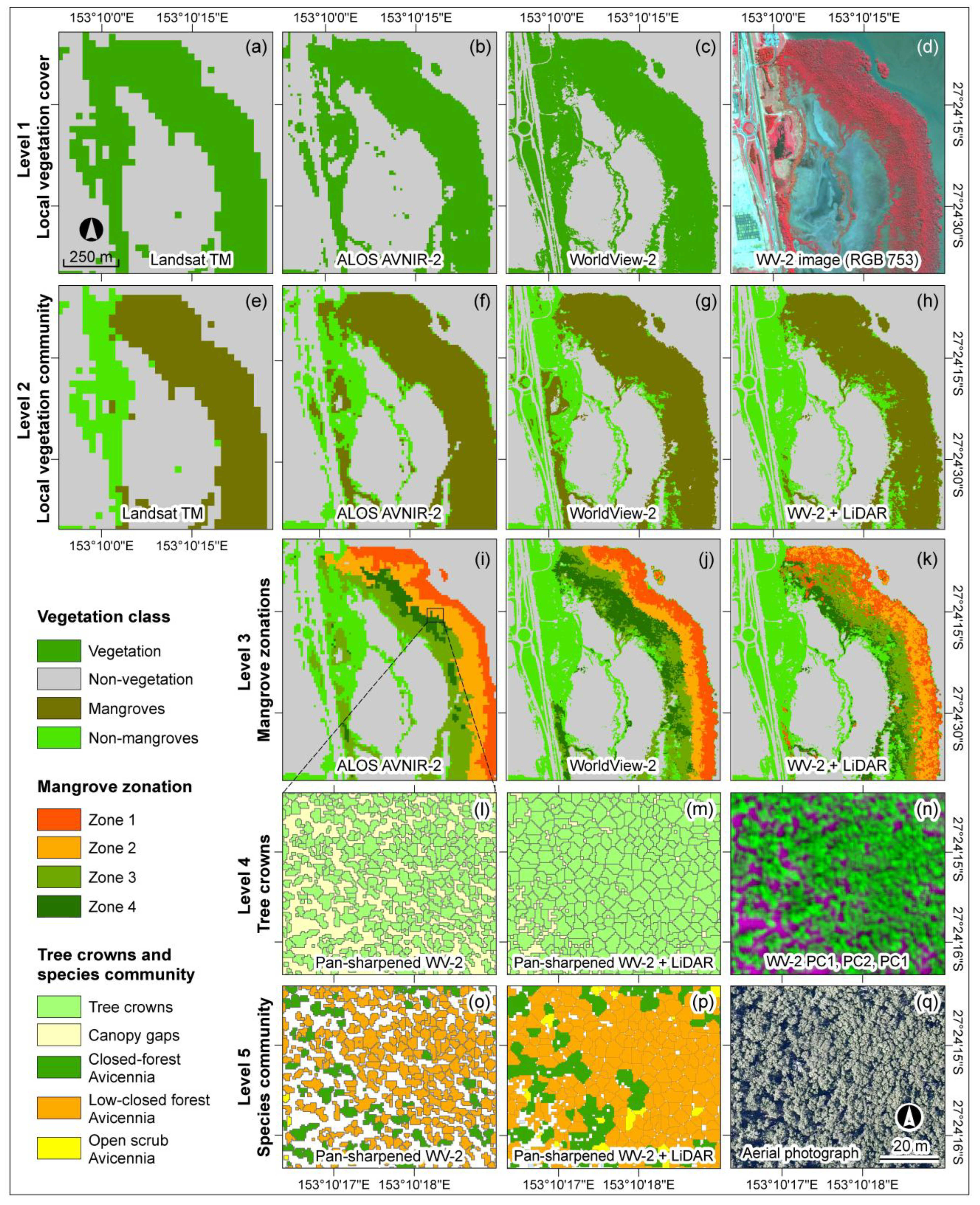
3.2. Mangrove Composition Maps

The results of our study demonstrated that the GEOBIA approach was able to produce various mangrove feature information details from a single and multiple images, by integrating the field data, operator local knowledge, and a conceptual hierarchical model of multi-scale mangrove features in the rule set (Figure 9). According to the semi-variogram results in Section 3.1, all the three Moreton Bay study sites were mapped at levels 1 to 3, but only mangroves at Whyte and Fisherman Islands were mapped in levels 4 and 5. The results showed that the developed rule set was able to map targeted mangrove composition objects from images with different spatial resolutions. Only limited studies have implemented the explicit hierarchical model of objects in mangrove mapping [9,12,16,69]. This study demonstrated the effectiveness of having a conceptual hierarchical model for mangrove mapping. It also described the ability and limitation of the images and the mapping approach in depicting information of mangrove composition. Nevertheless, membership rules/thresholds in the rule set required adjustment for each image (see Table 3). The results also show the required image pixel resolution aspect in the conceptual spatial hierarchical organization of mangroves features identifiable from remotely-sensed images (Figure 1).

Image spectral reflectance was the main criteria used to map vegetation and mangrove stands from the optical images (TM, AVNIR-2, and WV-2). The FDI algorithm successfully discriminated the vegetation and non-vegetation class (level 1) with a high degree of overall accuracy for TM (89%), AVNIR-2 (93%), and WV-2 (97%) (see Table 5 in Section 3.3). This pattern was also visually evident in Figure 9a to c, where the vegetation class boundary was more accurately represented in WV-2 than in the TM and AVNIR-2 images. The strip of Sarcocornia quinqueflora grass located in the middle of the saltmarsh was successfully mapped by WV-2 image (Figure 9c), but not by other images. We found the FDI algorithm was sensitive to all typical vegetation spectral reflectance, regardless how healthy the vegetation is. For example, the dry Sporobulus virginicus background grass, lacking the red-edge and absorption feature in the red part of the spectrum, which is typical for healthy green vegetation spectral reflectance [55,70] (Figure 5), was classified as vegetation. However, in general, the FDI algorithm was transferrable from WV-2 to the other images, but it required adjustment of the vegetation threshold for each image (Table 3).

We discriminated mangrove stands (level 2) within the vegetation class created in level 1. The spectral reflectance of mangroves is strongly influenced by tidal effects and soil background, resulting in mixed pixels [71,72]. As a consequence, it makes the application of a pixel-based approach in mangrove stands difficult. However, the combination of image bands and context information in the rule set in GEOBIA allows effective recognition of mangrove objects in the image [9,12,73]. For the spectral only approach, the green, red, NIR, and MIR bands provided a useful tool to discriminate mangrove stands from other vegetation objects. Exploratory work to find the best image band algorithm and associated threshold for each band, representing mangrove stands, suggested that each image has a unique combination of band algorithm and threshold to successfully separate mangroves from non-mangroves objects. However, the results showed some Casuarina glauca trees were misclassified as mangrove tree stands due to their similar spectral reflectance (see along the port highway in Figure 9e to g as examples). To refine the arbitrarily-defined spectral-based rule set, we included the DTM derived from LiDAR in the rule set as contextual information of the mangrove habitat. Based on the assessment of several DTM values, a threshold of DTM lower or equal to 1.5 m above mean sea level was found to be useful in combination with the WV-2 spectral-based rule set to separate mangroves with other terrestrial vegetation and applicable to all Moreton Bay mangrove sites. This additional contextual information significantly improved the accuracy of the mangrove delineation (Figure 9h) by 9% (Table 5).

Within the mangrove class, the zonation pattern in Moreton Bay was difficult to map using image spectral information only. The zonation pattern in Moreton Bay represents variations of Avicennia marina vegetation structure (i.e., canopy density, tree stem, tree height) across the mangrove stand. Hence, the mangrove zonation pattern differentiation based on image spectral reflectance suggested by Lucas et al. [56] was not applicable in this case. To address this issue, in theory, the inclusion of textural or contextual information might help the classification. However, we found that textural information of the image did not facilitate the zonation discrimination. It might be attributed to the fact that some of the mangrove zones have highly mixed vegetation structure stands with a number of canopy gaps (i.e., S3 and M4 in Moreton Bay), making it difficult to differentiate the zonation based on image texture. Instead, we used the distance from the coastline in combination with the spectral-based rule set to delineate each zone (Table 3), and this approach worked well (Figure 9i,j). We also investigated the use of the CHM and FCC derived from LiDAR data. The results showed that the mangrove zonation was oversimplified using the AVNIR-2 or WV-2 imagery, and well-represented using a combination of WV-2 and LiDAR data (Figure 9i–k, respectively). However, the accuracy assessment results suggested a low accuracy of the zonation maps. It was attributed to the inaccuracy in defining the mangrove zonation boundary, due to the mixed vegetation stands between zones.

The mangrove tree crowns and species community levels were mapped using pan-sharpened WV-2 image only (0.5 m) and a combination of pan-sharpened WV-2 with LiDAR data (2 m). Most of the mangrove tree canopies are very dense and have overlapping canopy arrangement. As a result, the definite borders of tree canopies were difficult to detect and delineate from the image. Therefore, to minimize the tree canopy border demarcation error, we developed a rule set that could (1) enhance the differentiation between canopy gaps and trees, and (2) find the tree crown seed and grow the seed towards the tree crown border within the tree class (Table 3). Figure 9n shows that PC band combination 1, 2 and 1 enhanced the differentiation of tree and canopy gaps. The tree crowns produced from the pan-sharpened WV-2 showed more realistic polygon boundaries compared to the result from the combination of pan-sharpened WV-2 and LiDAR data, with an overall accuracy of 68% and 64%, respectively (Table 5). Although LiDAR data provided a clear tree crown pattern along with the canopy height information, the optimum pixel resolution resampled from the point clouds was limited to 2 m. According to the result evaluation, the LiDAR data worked very well on large canopies (i.e., 8 m diameter or larger), but were unabled to depict small individual trees crown less than 8 m in diameter (see the result in comparison with Figure 9q). The LiDAR result in Figure 9m showed a very dense canopy with fewer and smaller canopy gaps compared to the pan-sharpened WV-2 result (Figure 9l). Therefore, as suggested by Gougeon [57] and Culvenor 59], high-spatial resolution image data with pixels significantly smaller than the tree canopy size is an essential requirement for tree crown delineation.

Figure 9. Example subsets of mangrove composition maps at Whyte Island, Moreton Bay, showing all hierarchy levels produced from different image sources: (a) level 1 TM, (b) level 1 AVNIR-2, (c) level 1 WV-2, (d) WV-2 image (RGB 753), (e) level 2 TM, (f) level 2 AVNIR-2, (g) level 2 WV-2, (h) level 2 WV-2+LiDAR, (i) level 3 AVNIR-2, (j) level 3 WV-2, (k) level 3 WV-2+LiDAR, (l) level 4 pan-sharpened WV-2, (m) level 4 pan-sharpened WV-2+LiDAR, (n) WV-2 PC1,2,1, (o) level 5 pan-sharpened WV-2, (p) level 5 pan-sharpened WV-2+LiDAR and (q) true color aerial photograph.

Figure 9. Example subsets of mangrove composition maps at Whyte Island, Moreton Bay, showing all hierarchy levels produced from different image sources: (a) level 1 TM, (b) level 1 AVNIR-2, (c) level 1 WV-2, (d) WV-2 image (RGB 753), (e) level 2 TM, (f) level 2 AVNIR-2, (g) level 2 WV-2, (h) level 2 WV-2+LiDAR, (i) level 3 AVNIR-2, (j) level 3 WV-2, (k) level 3 WV-2+LiDAR, (l) level 4 pan-sharpened WV-2, (m) level 4 pan-sharpened WV-2+LiDAR, (n) WV-2 PC1,2,1, (o) level 5 pan-sharpened WV-2, (p) level 5 pan-sharpened WV-2+LiDAR and (q) true color aerial photograph.

The mangrove species community maps were created based on the tree crown boundaries produced from the previous level. The NN algorithm successfully classified the Avicennia marina community. Visually, the map results follow the mangrove zonation pattern from the previous level. However, there were noticeable misclassified open scrub Avicennia in the WV-2 + LiDAR produced map. Although there was a clear difference pattern on the produced maps (Figure 9o and p), the results from the accuracy assessment did not show much difference between them (54% and 53%, respectively). The mangrove composition map produced by Queensland Herbarium has high details of thematic information. However, the coarse scale of the reference map (1:25,000), as opposed to the image resolution (0.5 and 2 m), was likely to be the source of this inaccuracy. The thematic information of the reference map was found to be useful for locating mangrove species communities, but not the boundary of the class.

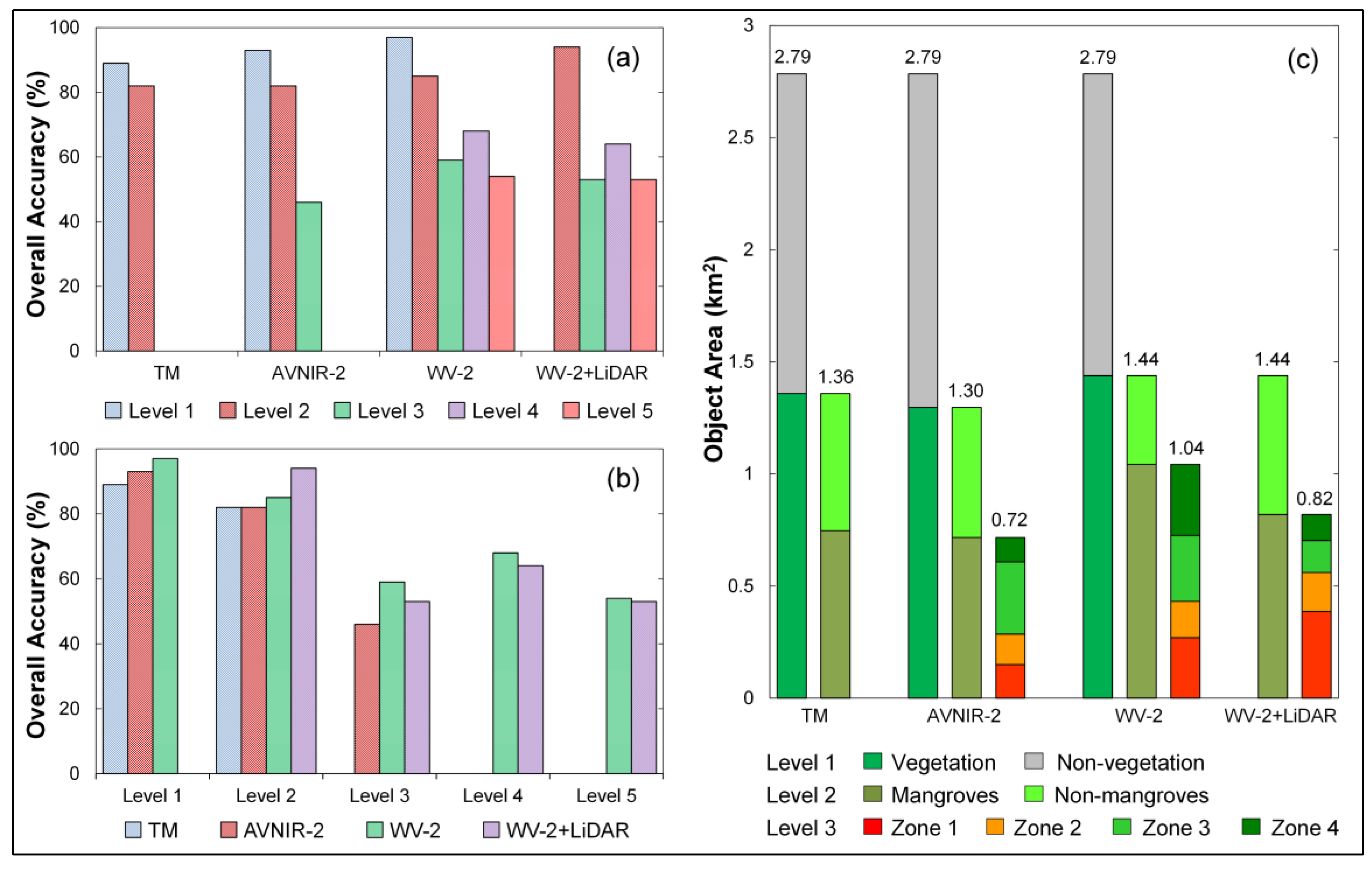
3.3. Accuracies, Errors and Uncertainties of the Maps

The main strength of this study was the high detection rate of mangrove features across the mapping levels. The area-based accuracy assessment calculated the area of the correctly classified class relative to the class domain area. In this study, we used an entire image for the domain area of level 1, vegetation class for level 2, and so on. Table 5 summarises the results of the area-based accuracy assessment descriptive statistics for all mangrove composition levels in this study. The overall quality (OQ) shows the class-related area accuracy; for instance, the area of correctly classified vegetation was 85% out of the total area of vegetation in level 1. On the other hand, the overall accuracy (OA) calculated the percentage of all correctly classified classes (vegetation and non-vegetation) in comparison to the total class domain area (an entire image).

Table 5. Summary of the area-based accuracy descriptive statistics in percentage (%).

Level	Class	Landsat TM				ALOS AVNIR-2				WorldView-2				WV2 + LiDAR
		OQ	PA	UA	OA	OQ	PA	UA	OA	OQ	PA	UA	OA	OQ	PA	UA	OA
1	Vegetation	85	92	92	89	90	93	97	93	95	99	97	97
	Non-vegetation	70	82	83		81	94	86		90	92	97
2	Mangroves	74	79	92	82	76	81	93	82	80	94	84	85	91	99	99	94
	Non-mangroves	66	88	72		66	85	75		63	69	88		87	98	97
3	Zone 1	-	-	-	-	55	57	92	46	72	75	96	53	72	75	95	59
	Zone 2	-	-	-	-	59	59	100		45	45	98		60	61	96
	Zone 3	-	-	-	-	38	38	99		49	50	97		39	39	99
	Zone 4	-	-	-	-	34	34	100		44	44	99		68	68	99
4										PS WV-2				PS WV-2 + LiDAR
	Tree crowns	-	-	-	-	-	-	-	-	64	81	76	68	56	64	82	64
	Canopy gaps	-	-	-	-	-	-	-	-	34	65	41		24	36	42
5	Avicennia (CF)	-	-	-	-	-	-	-	-	65	82	75	54	57	87	62	53
	Avicennia (LCF)	-	-	-	-	-	-	-	-	58	87	64		65	77	81
	Avicennia (OS)	-	-	-	-	-	-	-	-	22	23	94		4	4	20

OQ: overall quality, PA: producer’s accuracy, UA: user’s accuracy, OA: overall accuracy, PS: Pan-sharpened, CF: closed-forest, LCF: low closed-forest, OS: open scrub.

Table 5. Summary of the area-based accuracy descriptive statistics in percentage (%).

Level	Class	Landsat TM				ALOS AVNIR-2				WorldView-2				WV2 + LiDAR
		OQ	PA	UA	OA	OQ	PA	UA	OA	OQ	PA	UA	OA	OQ	PA	UA	OA
1	Vegetation	85	92	92	89	90	93	97	93	95	99	97	97
	Non-vegetation	70	82	83		81	94	86		90	92	97
2	Mangroves	74	79	92	82	76	81	93	82	80	94	84	85	91	99	99	94
	Non-mangroves	66	88	72		66	85	75		63	69	88		87	98	97
3	Zone 1	-	-	-	-	55	57	92	46	72	75	96	53	72	75	95	59
	Zone 2	-	-	-	-	59	59	100		45	45	98		60	61	96
	Zone 3	-	-	-	-	38	38	99		49	50	97		39	39	99
	Zone 4	-	-	-	-	34	34	100		44	44	99		68	68	99
4										PS WV-2				PS WV-2 + LiDAR
	Tree crowns	-	-	-	-	-	-	-	-	64	81	76	68	56	64	82	64
	Canopy gaps	-	-	-	-	-	-	-	-	34	65	41		24	36	42
5	Avicennia (CF)	-	-	-	-	-	-	-	-	65	82	75	54	57	87	62	53
	Avicennia (LCF)	-	-	-	-	-	-	-	-	58	87	64		65	77	81
	Avicennia (OS)	-	-	-	-	-	-	-	-	22	23	94		4	4	20

OQ: overall quality, PA: producer’s accuracy, UA: user’s accuracy, OA: overall accuracy, PS: Pan-sharpened, CF: closed-forest, LCF: low closed-forest, OS: open scrub.

The percentage of OQ and OA have similar pattern throughout the levels. For local mangrove features (levels 1 and 2), both OQ and OA have high accuracy levels, with increasing accuracy for the higher spatial resolution images (63%–95% and 82%–97%, respectively). It indicated the effectiveness of the mapping approach and the superiority of the high-spatial resolution images. The OQ and OA of “within mangrove features” (levels 3 to 5) showed lower accuracy levels (4%–72% and 46%–68%, respectively), suggesting that the rule set developed at these levels was unable to classify the targeted objects properly. Heumann [73] reported similar results, where the overall acuracy of mangrove stands was 94.4% and dropped to about 25% at mangrove species level. The producer’s accuracy (PA) depicts the omission error or the probability of a reference object being correctly classified, whereas the users’s accuracy (UA) or commission error indicates the probability of an object classified on the map actually represents that category on the ground [64]. For instance, for the delineation of tree crowns using the pan-sharpened WV-2 image, 81% of the tree crown areas was correctly classified as tree crown, but only 76% of the areas called tree crown on the map were actually tree crown on the ground.

Overall, the area-based accuracy assessment was simple to implement and easy to interpret. The result of this accuracy assessment approach was not only checking the thematic category of the object, but also representing the spatial accuracy of object boundaries compared to the reference. However, it calculated one class at a time [62] rather than all of the accuracy samples in one attempt, making the calculation more time-consuming. The locations of the areal sampling for calculation were also limited to the class domain area. Therefore, in accordance with the findings of Whiteside et al. [63], this may contribute to limiting the area sampled and hence included in the area-based accuracy assessment.

The main limitation of the mapping approach related to the classification rule set was its site, sensor and time dependency. This limitation was due to the spectral reflectance variations of the images captured by different sensors and the variations of the mangrove environmental settings. The rule set developed (i.e. algorithms and thresholds) was not directly transferrable to different sites, sensors and times of acquisition, and need to be modified accordingly. The only uncertainties introduced in the accuracy assessment were attributed to the time gap of one and three years between the image and field data acquisition times for Moreton Bay and Karimunjawa Island, respectively. Some level of change in mangrove condition may have occurred within these time gaps. However, we notice that there was no major disturbance (such as flood, tsunami, cyclone and logging) affecting the study areas within the time gaps.

3.4. Multi-Scale Mangrove Composition Mapping

The effects of the L- and H-resolution model of remote sensing data [74] to the produced mangrove maps were evident in this study. The results indicated that low-resolution images have limited ability to depict mangrove features compared to the high-resolution images (Figure 9). The TM image (30 m) was only able to differentiate mangrove stand objects (Figure 9e); and the AVNIR-2 (10 m) and WV-2 images (2 m) were able to map different mangrove zonation patterns (Figure 9i and j). The pan-sharpened WV-2 (0.5 m) and LiDAR, on the other hand, were able to map more detailed mangrove features to the level of mangrove tree crowns and species communities (Figure 9l to 9o). A decrease in image spatial resolution affects spectral heterogeneity of the image since it creates mixed pixels [27,74] hence being less sensitive to the spatial complexity and hampers the ability to discriminate small objects relative to the pixel size [74,75].

The comparison of overall accuracy per image (Figure 10a) indicated that WV-2 imagery has the highest overall accuracy for all of the levels. For levels 1 and 2 there were a clear increase of accuracy when increasing image spatial resolution. Levels 3 to 5 also confirmed this pattern. The decrease of overall accuracy when combining WV-2 and LiDAR data was attributed to the 2 m resampling of LiDAR point cloud. Yet, it is important to note that a comparatively large number of spectral bands available with a limited spectral range for the WV-2 image also enabled more flexibility in applying the GEOBIA rule set [12]. Increasing in spectral resolution provides additional explanatory information in object recognition [75], which in turn increases the classification accuracy.

Figure 10. Comparison of the overall accuracy result of (a) different images and (b) different levels, and (c) area of the produced maps for level 1, 2, and 3 in Whyte Island, Moreton Bay.

Figure 10. Comparison of the overall accuracy result of (a) different images and (b) different levels, and (c) area of the produced maps for level 1, 2, and 3 in Whyte Island, Moreton Bay.

Looking at the variation across levels, the overall accuracy decreased by increasing of the mapping level (i.e., finer scale or smaller object size) (Figure 10b). There are several possible explanations for this pattern. First, smaller object sizes (i.e., zonations, tree crowns, and individual species) required more complex classification rule sets to map the land-cover classes. The inaccurate definition of the rule set will affect the accuracy of the mapping. Second, smaller object sizes increase within-class variability, which decreases the spectral separability of classes and potentially decrease the accuracy [76,77]. This effect is well-known in pixel-based approaches [75] and may also affect the GEOBIA approach. Third, it is suggested that a higher number of thematic classes used in the classification tends to reduce the accuracy of the results [78,79]. A larger number of targeted land-cover classes requires a more complex definition of each object category for effective separation, and increase the “boundary effect” [77]. As the targeted objects become smaller, the proportion of segments falling on the boundary of objects will increase and hence potentially decrease the mapping accuracy. The object area comparison in Figure 10c showed that the area difference of land-cover classes between images (indicated by the numbers on top of the bar graph) was increased by the increasing number of targeted object classes. At level 1 the area was similar across images. At levels 2 and 3 the area increased by to 0.14 and 0.32 km², respectively. The relatively large area of mangroves mapped from WV-2 image was attributed to the decreasing boundary effect due to the high-spatial resolution of the image.

3.5. Applicability of the Approach to Other Sites

The next question following the success of the implementation of the mapping approach is whether the approach can be applied elsewhere. Developing an approach or algorithm that can be universally implemented is one of the major challenges in remote sensing applications. Unfortunately, this situation is difficult to achieve and rarely happen because of varying environmental conditions, seasonality, sensor viewing geometry, level of pre-processing, spatial resolution and image sensor types. Most of the mapping procedures and algorithms employing remote sensing data are site and sensor specific. We investigated the transferability of the conceptual hierarchical model of multi-scale mangrove features and its rule set to another site on Karimunjawa Island using the same image datasets (TM, AVNIR-2, and WV-2). All image datasets were pre-processed to the same level using the same correction methods, to ensure a fair comparison.

In theory, the conceptual hierarchical model developed indicates the “domains of scale” [17] of mangrove features and provides logical multi-scale mapping guideline, that can be applied everywhere. However, when it comes down to the technical mapping aspect, the result might be unexpected. We found that only the three first hierarchical levels could be mapped. This limitation was in accordance with the results of mangrove spatial pattern analysis discussed in Section 3.1 (Figure 8). According to field observations, mangroves on Karimunjawa Island are richer in species composition, have higher canopy density, and consist of taller and more matured trees as opposed to Moreton Bay mangroves. The dense and highly overlapping tree canopies prevented the delineation of the individual tree crowns. Therefore, the difference of environmental settings and local variation of mangrove composition affected the implementation of the model.

A direct transfer of the rule set from Moreton Bay to Karimunjawa Island was not possible. At level 1, the FDI algorithm successfully discriminated vegetation and non-vegetation objects from all of the images, but required modification in the membership thresholds. Mangrove and non-mangrove separation and mangrove zonation delineation were performed using different processes and membership rules in the rule set compared to the Moreton Bay site. Apart from the environmental setting, the canopy reflectance depends on a numbers of factors and varied across location and time [80]. Thus, the image spectral response might also contribute to the rule set modification requirements.

4. Conclusions and Future Research

This study compared and contrasted the ability of different image datasets (Landsat TM, ALOS AVNIR-2, WorldView-2, LiDAR) to map five levels of mangrove features, including vegetation boundaries, mangrove stands, mangrove zonations, individual tree crowns, and species communities. We used Moreton Bay in Australia as the primary site to develop the classification rule sets and Karimunjawa Island in Indonesia to test the applicability of the rule sets. This study was the first attempt to develop and implement a conceptual spatial and temporal hierarchical organization of mangroves for mangrove feature mapping at multiple scales. The results demonstrated that scale-specific, ecologically relevant information on mangroves can be effectively mapped using a conceptual hierarchical model of multi-scale mangrove features implemented through the rule sets in GEOBIA. For mangrove and non-mangrove mapping, the use of TM, AVNIR-2, WV-2 and WV-2 + LiDAR data provided overall accuracies of 82%, 82%, 85%, and 94%, respectively. The results suggest that higher spatial resolution images are required to map detailed information of mangroves. The TM image was only able to differentiate mangrove stand objects, while AVNIR-2 and WV-2 imagery allowed different mangrove zonation patterns to be mapped. The pan-sharpened WV-2 and LiDAR data could be used to map more detailed mangrove features, including individual mangrove tree crowns and species communities. However, we also noted that the superiority of WV-2 imagery was also attributed to the relatively large number of spectral bands.

Developing an efficient rule set requires an understanding of the spectral, physical, and contextual characteristics of the targeted object(s). We found that the inclusion of contextual information, in the form of elevation and distance, significantly increased the accuracy of the mapping. However, the development of rule sets is image and site dependent. Different algorithms and threshold values might be applied to different images to map similar objects due to variation of object spectral reflectance responses between images. Modification of algorithms and membership thresholds was also needed to map similar object at different locations, due to the different environmental settings, local mangrove composition variation, and the site-specific spectral response. We found that the accuracy of maps was defined by interactions between image spatial resolution, the scale of the targeted objects, and the number of object land-cover classes mapped. Although it is achievable using high-resolution images, mapping smaller objects required a more complex rule set to be developed due to increase within-class variability that potentially decreases the mapping accuracy. Incorporation of a larger number of object categories adds more complexity of class definition and increases the boundary effect, which in turn will decrease the mapping accuracy.

The findings of this study provide a conceptual guidance of multi-scale mangrove mapping and a technical demonstration to produce scale-specific mangrove information. This information is essential to address mangrove ecological problems at a relevant spatial scale. Hence, this research builds a fundamental approach for multi-scale mangrove mapping and advances the current knowledge on and the application of GEOBIA for mangrove mapping. However, the results of this study were limited to the selected images, mapping techniques, and mangrove sites. Further research need to include a wider range of images and mapping techniques. The potential of including image texture in high-spatial resolution image also needs to be explored further. Finally, to ensure the transferability of the conceptual hierarchical model, this approach needs to be tested at locations rich in mangrove species with distinctive individual tree canopies.

References

1. Giri, C.; Pengra, B.; Zhu, Z.; Singh, A.; Tieszen, L.L. Monitoring mangrove forest dynamics of the Sundarbans in Bangladesh and India using multi-temporal satellite data from 1973 to 2000. Estuar. Coast. Shelf Sci. 2007, 73, 91–100. [Google Scholar] [CrossRef]
2. Green, E.P.; Mumby, P.J.; Edwards, A.J.; Clark, C.D.; Ellis, A.C. The assessment of mangrove areas using high resolution multispectral airborne imagery. J. Coast. Res. 1998, 14, 433–443. [Google Scholar]
3. Green, E.P.; Clark, C.D.; Mumby, P.J.; Edwards, A.J.; Ellis, A.C. Remote sensing techniques for mangrove mapping. Int. J. Remote Sens. 1998, 19, 935–956. [Google Scholar] [CrossRef]
4. Davis, B.A.; Jensen, J.R. Remote sensing of mangrove biophysical characteristics. Geocarto Int. 1998, 13, 55–64. [Google Scholar] [CrossRef]
5. Hardisky, M.A.; Gross, M.F.; Klemas, V. Remote sensing of coastal wetlands. BioScience 1986, 36, 453–460. [Google Scholar] [CrossRef]
6. Malthus, T.J.; Mumby, P.J. Remote sensing of the coastal zone: An overview and priorities for future research. Int. J. Remote Sens. 2003, 24, 2805–2815. [Google Scholar] [CrossRef]
7. Giri, C.; Ochieng, E.; Tieszen, L.L.; Zhu, Z.; Singh, A.; Loveland, T.; Masek, J.; Duke, N. Status and distribution of mangrove forests of the world using earth observation satellite data. Glob. Ecol. Biogeogr. 2011, 20, 154–159. [Google Scholar] [CrossRef]
8. Bhattarai, B.; Giri, C. Assessment of mangrove forests in the Pacific region using Landsat imagery. J. Appl. Remote Sens. 2011, 5, 053509–053511. [Google Scholar] [CrossRef]
9. Kamal, M.; Phinn, S.R. Hyperspectral data for mangrove species mapping: A comparison of pixel-based and object-based approach. Remote Sens. 2011, 3, 2222–2242. [Google Scholar] [CrossRef]
10. Wang, L.; Sousa, W.P.; Gong, P.; Biging, G.S. Comparison of IKONOS and QuickBird images for mapping mangrove species on the Caribbean coast of Panama. Remote Sens. Environ. 2004, 91, 432–440. [Google Scholar] [CrossRef]
11. Koedsin, W.; Vaiphasa, C. Discrimination of tropical mangroves at the species level with EO-1 Hyperion data. Remote Sens. 2013, 5, 3562–3582. [Google Scholar] [CrossRef]
12. Heenkenda, M.; Joyce, K.; Maier, S.; Bartolo, R. Mangrove species identification: Comparing WorldView-2 with aerial photographs. Remote Sens. 2014, 6, 6064–6088. [Google Scholar] [CrossRef]
13. Heumann, B.W. Satellite remote sensing of mangrove forests: Recent advances and future opportunities. Progress Phys. Geogr. 2011, 35, 87–108. [Google Scholar] [CrossRef]
14. Kuenzer, C.; Bluemel, A.; Gebhardt, S.; Quoc, T.V.; Dech, S. Remote sensing of mangrove ecosystems: A review. Remote Sens. 2011, 3, 878–928. [Google Scholar] [CrossRef]
15. Held, A.; Ticehurst, C.; Lymburner, L.; Williams, N. High resolution mapping of tropical mangrove ecosystems using hyperspectral and radar remote sensing. Int. J. Remote Sens. 2003, 24, 2739–2759. [Google Scholar] [CrossRef]
16. Krause, G.; Bock, M.; Weiers, S.; Braun, G. Mapping land-cover and mangrove structures with remote sensing techniques: A contribution to a synoptic GIS in support of coastal management in North Brazil. Environ. Manag. 2004, 34, 429–440. [Google Scholar] [CrossRef]
17. Wiens, J.A. Spatial scaling in ecology. Funct. Ecol. 1989, 3, 385–397. [Google Scholar] [CrossRef]
18. Marceau, D.J.; Hay, G.J. Remote sensing contributions to the scale issue. Can. J. Remote Sens. 1999, 25, 357–366. [Google Scholar] [CrossRef]
19. Schaeffer-Novelli, Y.; Cintrón-Molero, G.; Cunha-Lignon, M.; Coelho, C., Jr. A conceptual hierarchical framework for marine coastal management and conservation: A “Janus-like” approach. J. Coast. Res. 2005, 42, 191–197. [Google Scholar]
20. Farnsworth, E.J. Issues of spatial, taxonomic and temporal scale in delineating links between mangrove diversity and ecosystem function. Glob. Ecol. Biogeogr. Lett. 1998, 7, 15–25. [Google Scholar] [CrossRef]
21. Twilley, R.R.; Rivera-Monroy, V.H.; Chen, R.; Botero, L. Adapting an ecological mangrove model to simulate trajectories in restoration ecology. Marine Pollut. Bull. 1999, 37, 404–419. [Google Scholar] [CrossRef]
22. Duke, N.C.; Ball, M.C.; Ellison, J.C. Factors influencing biodiversity and distributional gradients in mangroves. Glob. Ecol. Biogeogr. Lett. 1998, 7, 27–47. [Google Scholar] [CrossRef]
23. Feller, I.C.; Lovelock, C.E.; Berger, U.; McKee, K.L.; Joye, S.B.; Ball, M.C. Biocomplexity in mangrove ecosystems. Ann. Rev. Marine Sci. 2010, 2, 395–417. [Google Scholar] [CrossRef]
24. Burnett, C.; Blaschke, T. A multi-scale segmentation/object relationship modelling methodology for landscape analysis. Ecol. Model. 2003, 168, 233–249. [Google Scholar] [CrossRef]
25. Blaschke, T.; Hay, G.J.; Kelly, M.; Lang, S.; Hofmann, P.; Addink, E.; Queiroz Feitosa, R.; van der Meer, F.; van der Werff, H.; van Coillie, F.; et al. Geographic object-based image analysis—Towards a new paradigm. ISPRS J. Photogramm. Remote Sens. 2014, 87, 180–191. [Google Scholar] [CrossRef] [PubMed]
26. Blaschke, T. Multiscale image analysis for ecological monitoring of heterogeneous, small structured landscapes. Proc. SPIE 2002, 4545, 35–44. [Google Scholar]
27. Woodcock, C.E.; Strahler, A.H. The factor of scale in remote sensing. Remote Sens. Environ. 1987, 21, 311–332. [Google Scholar] [CrossRef]
28. Woodcock, C.; Harward, V.J. Nested-hierarchical scene models and image segmentation. Int. J. Remote Sens. 1992, 13, 3167–3187. [Google Scholar] [CrossRef]
29. Berger, U.; Rivera-Monroy, V.H.; Doyle, T.W.; Dahdouh-Guebas, F.; Duke, N.C.; Fontalvo-Herazo, M.L.; Hildenbrandt, H.; Koedam, N.; Mehlig, U.; Piou, C.; et al. Advances and limitations of individual-based models to analyze and predict dynamics of mangrove forests: A review. Aquat. Bot. 2008, 89, 260–274. [Google Scholar] [CrossRef]
30. Kamal, M.; Phinn, S.; Johansen, K. Characterizing the spatial structure of mangrove features for optimizing image-based mangrove mapping. Remote Sens. 2014, 6, 984–1006. [Google Scholar] [CrossRef]
31. Blaschke, T.; Strobl, J. What’s wrong with pixels? Some recent development interfacing remote sensing and GIS. GeoBIT/GIS 2001, 6, 12–17. [Google Scholar]
32. Müller, F. State-of-the-art in ecosystem theory. Ecol. Model. 1997, 100, 135–161. [Google Scholar] [CrossRef]
33. Castilla, G.; Hay, G.J. Image objects and geographic objects. In Object-Based Image Analysis: Spatial Concepts for Knowledge-Driven Remote Sensing Applications; Blaschke, T., Lang, S., Hay, G.J., Eds.; Springer-Verlag: Berlin, Germany, 2008; pp. 93–112. [Google Scholar]
34. Gamanya, R.; de Maeyer, P.; de Dapper, M. An automated satellite image classification design using object-oriented segmentation algorithms: A move towards standardization. Expert Syst. Appl. 2007, 32, 616–624. [Google Scholar] [CrossRef]
35. Blaschke, T. Object based image analysis for remote sensing. ISPRS J. Photogramm. Remote Sens. 2010, 65, 2–16. [Google Scholar] [CrossRef]
36. Hay, G.J.; Castilla, G.; Wulder, M.A.; Ruiz, J.R. An automated object-based approach for the multiscale image segmentation of forest scenes. Int. J. Appl. Earth Obs. Geoinf. 2005, 7, 339–359. [Google Scholar] [CrossRef]
37. Johansen, K.; Phinn, S.; Witte, C.; Philip, S.; Newton, L. Mapping banana plantations from object-oriented classification of SPOT-5 imagery. Photogramm. Eng. Remote Sens. 2009, 75, 1069–1081. [Google Scholar] [CrossRef]
38. Environment Australia. A Directory of Important Wetlands in Australia, 3rd ed.; Environment Australia: Canberra, Australia, 2001; p. 157. [Google Scholar]
39. Dowling, R.M.; Stephen, K. Coastal Wetlands of South-Eastern Queensland Maroochy Shire to New South Wales Border; Queensland Herbarium, Environmental Protection Agency: Brisbane, Australia, 2001; p. 220. [Google Scholar]
40. Duke, N. Australia’s Mangroves: The Authoritative Guide to Australia’s Mangrove Plants; University of Queensland: Brisbane, Australia, 2006; p. 200. [Google Scholar]
41. Balai Taman Nasional Karimunjawa (BTNK). terpretasi Trekking Mangrove Taman Nasional Karimunjawa; Balai Taman Nasional Karimunjawa: Semarang, Indonesia, 2011; p. 24. [Google Scholar]
42. LAADS Level 1 and Atmosphere Archive and Distribution System. Website of NASA—Goddard Space Flight Center. Available online: http://ladsweb.nascom.nasa.gov/data/search.html (accessed on 5 March 2012).
43. Laben, C.A.; Brower, B.V. Process for Enhancing the Spatial Resolution of Multispectral Imagery Using Pan-Sharpening. US6011875 A, 4 January 2000. [Google Scholar]
44. Specht, R.L.; Specht, A.; Whelan, M.B.; Hegarty, E.E. Conservation Atlas of Plant Communities in Australia; Southern Cross University Press: Lismore, Australia, 1995; p. 910. [Google Scholar]
45. Kitamura, S.; Anwar, C.; Chaniago, A.; Baba, S. Handbook of Mangroves in Indonesia: Bali & Lombok; International Society of mangrove Ecosystem (ISME): Okinawa, Japan, 2004. [Google Scholar]
46. Woodcock, C.E.; Strahler, A.H.; Jupp, D.L.B. The use of variograms in remote sensing: I. Scene models and simulated images. Remote Sens. Environ. 1988, 25, 323–348. [Google Scholar] [CrossRef]
47. Curran, P.J.; Atkinson, P.M. Geostatistics and remote sensing. Progress Phys. Geogr. 1998, 22, 61–78. [Google Scholar] [CrossRef]
48. Cohen, W.B.; Spies, T.A.; Bradshaw, G.A. Semivariograms of digital imagery for analysis of conifer canopy structure. Remote Sens. Environ. 1990, 34, 167–178. [Google Scholar] [CrossRef]
49. Johansen, K.; Phinn, S. Linking riparian vegetation spatial structure in Australian tropical savannas to ecosystem health indicators: Semi-variogram analysis of high spatial resolution satellite imagery. Can. J. Remote Sens. 2006, 32, 228–243. [Google Scholar] [CrossRef]
50. de Jong, S.M.; van der Meer, F.D. Remote Sensing Image Analysis: Including the Spatial Domain; Kluwer Academic Publishers: Dordrecht, The Netherlands, 2005; p. 359. [Google Scholar]
51. Hay, G.J.; Blaschke, T.; Marceau, D.J.; Bouchard, A. A comparison of three image-object methods for the multiscale analysis of landscape structure. ISPRS J. Photogramm. Remote Sens. 2003, 57, 327–345. [Google Scholar] [CrossRef]
52. Trimble. eCognition Developer 8.7 User Guide; TrimbleGermany GmbH: Munchen, Germany, 2011; p. 258. [Google Scholar]
53. Baatz, M.; Schäpe, A. Object-oriented and multi-scale image analysis in semantic networks. In Proceedings of 2nd International Symposium on Operationalization of Remote Sensing, ITC, The Netherland, 16–20 August 1999.
54. Wu, J. Hierarchy and scaling: Extrapolating information along a scaling ladder. Can. J. Remote Sens. 1999, 25, 367–380. [Google Scholar] [CrossRef]
55. Bunting, P.; Lucas, R. The delineation of tree crowns in Australian mixed species forests using hyperspectral Compact Airborne Spectrographic Imager (CASI) data. Remote Sens. Environ. 2006, 101, 230–248. [Google Scholar] [CrossRef]
56. Lucas, R.M.; Mitchell, A.L.; Rosenqvist, A.; Proisy, C.; Melius, A.; Ticehurst, C. The potential of L-band SAR for quantifying mangrove characteristics and change: Case studies from the tropics. Aquat. Conserv. 2007, 17, 245–264. [Google Scholar] [CrossRef]
57. Gougeon, F.A. A crown-following approach to the automatic delineation of individual tree crowns in high spatial resolution aerial images. Can. J. Remote Sens. 1995, 21, 274–284. [Google Scholar] [CrossRef]
58. Culvenor, D.S. TIDA: An algorithm for the delineation of tree crowns in high spatial resolution remotely sensed imagery. Comput. Geosci. 2002, 28, 33–44. [Google Scholar] [CrossRef]
59. Culvenor, D.S. Extracting individual tree information: A survey of techniques for high spatial resolution imagery. In Remote Sensing of Forest Environments: Concepts and Case Studies; Wulder, M.A., Franklin, S.E., Eds.; Kluwer Academic Publishers: Boston, MA, USA, 2003; pp. 255–277. [Google Scholar]
60. Gougeon, F.A.; Leckie, D.G. The individual tree crown approach applied to IKONOS images of a coniferous plantation area. Photogramm. Eng. Remote Sens. 2006, 72, 1287–1297. [Google Scholar] [CrossRef]
61. Schopfer, E.; Lang, S. Object fate analysis—A virtual overlay method for the categorisation of object transition and object-based accuracy assessment. In Proceedings of 1st International Conference on Object-based Image Analysis (OBIA 2006), Salzburg, Austria, 4–5 July 2006.
62. Zhan, Q.; Molenaar, M.; Tempfli, K.; Shi, W. Quality assessment for geo-spatial objects derived from remotely sensed data. Int. J. Remote Sens. 2005, 26, 2953–2974. [Google Scholar] [CrossRef]
63. Whiteside, T.; Boggs, G.; Maier, S. Area-based validity assessment of single- and multi-class object-based image analysis. In Proceedings of 15th Australasian Remote Sensing and Photogrammetry Conference, Alice Spring, Australia, 13–17 September 2010.
64. Congalton, R.G. A review of assessing the accuracy of classifications of remotely sensed data. Remote Sens. Environ. 1991, 37, 35–46. [Google Scholar] [CrossRef]
65. Dowling, R.; Stephens, K. Coastal Wetlands of South East Queensland: Volume 1 Mapping and Survey; Queensland Herbarium: Brisbane, Australia, 1998. [Google Scholar]
66. Jupp, D.L.B.; Strahler, A.H.; Woodcock, C.E. Autocorrelation and regularization in digital images. II. Simple image models. IEEE Trans. Geosci. Remote Sens. 1989, 27, 247–258. [Google Scholar] [CrossRef]
67. Woodcock, C.E.; Strahler, A.H.; Jupp, D.L.B. The use of variograms in remote sensing: II. Real digital images. Remote Sens. Environ. 1988, 25, 349–379. [Google Scholar] [CrossRef]
68. Curran, P.J. The semivariogram in remote sensing: An introduction. Remote Sens. Environ. 1988, 24, 493–507. [Google Scholar] [CrossRef]
69. Murray, M.R.; Zisman, S.A.; Furley, P.A.; Munro, D.M.; Gibson, J.; Ratter, J.; Bridgewater, S.; Minty, C.D.; Place, C.J. The mangroves of Belize: Part 1. distribution, composition and classification. Forest Ecol. Manag. 2003, 174, 265–279. [Google Scholar] [CrossRef]
70. Carter, G.A. Ratios of leaf reflectances in narrow wavebands as indicators of plant stress. Int. J. Remote Sens. 1994, 15, 697–703. [Google Scholar] [CrossRef]
71. Blasco, F.; Gauquelin, T.; Rasolofoharinoro, M.; Denis, J.; Aizpuru, M.; Caldairou, V. Recent advances in mangrove studies using remote sensing data. Mar. Freshwater Res. 1998, 49, 287–296. [Google Scholar] [CrossRef]
72. Díaz, B.M.; Blackburn, G.A. Remote sensing of mangrove biophysical properties: Evidence from a laboratory simulation of the possible effects of background variation on spectral vegetation indices. Int. J. Remote Sens. 2003, 24, 53–73. [Google Scholar] [CrossRef]
73. Heumann, B.W. An object-based classification of mangroves using a hybrid decision tree—Support Vector Machine approach. Remote Sens. 2011, 3, 2440–2460. [Google Scholar] [CrossRef]
74. Strahler, A.H.; Woodcock, C.E.; Smith, J.A. On the nature of models in remote sensing. Remote Sens. Environ. 1986, 20, 121–139. [Google Scholar] [CrossRef]
75. Rocchini, D. Effects of spatial and spectral resolution in estimating ecosystem α-diversity by satellite imagery. Remote Sens. Environ. 2007, 111, 423–434. [Google Scholar] [CrossRef]
76. Chusnie, J.L. The interactive effect of spatial resolution and degree of internal variability within land-cover types on classification accuracies. Int. J. Remote Sens. 1987, 8, 15–29. [Google Scholar] [CrossRef]
77. Markham, B.L.; Townshend, J.R.G. Land cover classification accuracy as a function of sensor spatial resolution. In Proceedings of the 15th International Symposium on Remote Sensing of Environment, Ann Arbor, MI, USA, 11–15 May 1981.
78. Andrefouet, S.; Kramer, P.; Torres-Pulliza, D.; Joyce, K.E.; Hochberg, E.J.; Garza-Pe´rez, R.; Mumby, P.J.; Riegl, B.; Yamano, H.; White, W.H.; et al. Multi-site evaluation of IKONOS data for classification of tropical coral reef environments. Remote Sens. Environ. 2003, 88, 128–143. [Google Scholar] [CrossRef]
79. Roelfsema, C.M.; Phinn, S.R. Validation. In Coral Reef Remote Sensing; Goodman, J.A., Purkis, S.J., Phinn, S.R., Eds.; Springer: Dordrecht, The Netherlands, 2013; pp. 375–401. [Google Scholar]
80. Atzberger, C. Object-based retrieval of biophysical canopy variables using artificial neural nets and radiative transfer models. Remote Sens. Environ. 2004, 93, 53–67. [Google Scholar] [CrossRef]