Surface Shortwave Net Radiation Estimation from FengYun-3 MERSI Data

Abstract

The Medium-Resolution Spectral Imager (MERSI) is one of the major payloads of China’s second-generation polar-orbiting meteorological satellite, FengYun-3 (FY-3), and it is similar to the Moderate-Resolution Imaging Spectroradiometer (MODIS). The MERSI data are suitable for mapping terrestrial, atmospheric and oceanographic variables at continental to global scales. This study presents a direct-estimation method to retrieve surface shortwave net radiation (SSNR) data from MERSI top-of-atmosphere (TOA) reflectance and cloud mask products. This study is the first attempt to use the MERSI to retrieve SSNR data. Several critical issues concerning remote sensing of SSNR were investigated, including scale effects in validating SSNR data, impacts of the MERSI calibration update on the estimation of SSNR and the dependency of the retrieval accuracy of SSNR data on view geometry. We also incorporated data from twin MODIS sensors to assess how time and the number of satellite overpasses affect the retrieval of SSNR data. Validation against one-year data over seven Surface Radiation Budget Network (SURFRAD) stations showed that the presented algorithm estimated daily SSNR at the original resolution of the MERSI with a root mean square error (RMSE) of 41.9 W/m² and a bias of −1.6 W/m². Aggregated to a spatial resolution of 161 km, the RMSE of MERSI retrievals can be reduced by approximately 10 W/m². Combined with MODIS data, the RMSE of daily SSNR estimation can be further reduced to 22.2 W/m². Compared with that of daily SSNR, estimation of monthly SSNR is less affected by the number of satellite overpasses per day. The RMSE of monthly SSNR from a single MERSI sensor is as small as 13.5 W/m².

1. Introduction

Surface shortwave net radiation (SSNR), calculated as the difference between surface incident shortwave radiation and the amount of radiation reflected back into the atmosphere by the surface, is a function of both atmospheric and surface properties, in addition to solar elevation angle [1,2]. It largely determines the total net radiation [3]. Traditional approaches of retrieving SSNR data from satellite data involve separate estimation of incident solar radiation and surface broadband albedo [4]. Recently, SSNR has also been directly estimated from top-of-atmosphere (TOA) reflectance acquired by various sensors, including the Landsat Thematic Mapper (TM) [5], the Moderate-Resolution Imaging Spectroradiometer (MODIS) [6] and the Airborne Visible Infrared Imaging Spectrometer (AVIRIS) [7]. Typically, such SSNR data retrievals are instantaneous values at the imagery acquiring time. However, studies of the surface radiation budget usually need the mean SSNR for a period of time (e.g., daily or monthly), rather than instantaneous SSNR at a specific time. Estimating daily SSNR from a limited number of satellite observations within a day involves interpolating atmospheric conditions from the observation times to the entire day. Assuming stable atmospheric conditions, Wang and Liang expanded the direct-estimation method for instantaneous SSNR and estimated daily SSNR from a single Landsat TM observation [5]. The major drawback of this method is that it fails to consider the intra-daily variations of atmospheric conditions, such as aerosol loading, cloud coverage and water vapor concentration. Recently, they further refined the algorithm by considering variations in view angles and improving simulations of radiative transfer with more representative aerosol and cloud types [8]. The improved algorithm was applied over the combined MODIS data from Terra and Aqua to generate daily SSNR data with substantially improved accuracy.

Similar to NASA’s MODIS, the Medium-Resolution Spectral Imager (MERSI) is a moderate-resolution multispectral radiometer operated by the China Meteorological Administration [9]. It is one of the major payloads of the FengYun (FY)-3 series, China’s polar-orbiting meteorological satellites. The MERSI comprises 19 reflective solar bands (RSBs) and one thermal emissive band (TEB). The first five bands, including four RSBs and the TEB, have a nadir spatial resolution of 250 m. The resolution of the remaining 15 bands is 1 km. This type of medium-resolution optical sensor is ideal for mapping environmental and climate variables, such as SSNR at the continental or global scales, because of their global coverage, short revisiting intervals, ample spectral information and moderate data volume. In addition to data of TOA radiance and reflectance, several high-level products are derived from MERSI data, including cloud mask, aerosol over ocean and land, ocean color, precipitable water, land cover and vegetation indices (Normalized Difference Vegetation Index (NDVI) and Enhanced Vegetation Index (EVI)) [10]. However, data of the surface radiative fluxes, including SSNR, are not currently produced from MERSI data. In this study, we adopted the direct-estimation method for MODIS data to retrieve daily SSNR from MERSI observations. As far as we know, this is the first attempt to use China’s MERSI data to retrieve SSNR. Several critical issues on remote sensing of SSNR were investigated in the study, including scale effects in validating SSNR, the impacts of MERSI’s calibration update on estimating high level products and the dependency of the retrieval accuracy of SSNR on view geometry. We also incorporated data from twin MODIS sensors to assess how the timing and count of observations affect the retrieval of daily SSNR. The paper is organized as follows. Section 2 briefly introduces the MERSI and its radiometric calibration. Section 3 reviews the direct-estimation algorithm. Section 4 presents the results and discussion. Section 5 concludes the paper by summarizing the major findings.

2. MERSI Data

A total of three FY-3 satellites are currently in operation, namely FY-3A, FY-3B and FY-3C, launched on 27 May 2008, 10 November 2010 and 23 September 2013, respectively. To reduce the data volume, only MERSI data from FY-3B are considered in the study. Annual data for 2013 over Surface Radiation Budget Network (SURFRAD) sites were obtained. The SURFRAD network consists of seven sites with a range of land cover types, including cropland, grassland, forest and desert. Downward and upward shortwave irradiances are measured every minute at these sites. A daily value of SSNR is calculated as the mean of the difference between downward and upward shortwave irradiances of the day [8]. To study the dependency of retrieval accuracy on spatial resolutions, a window of 300 by 300 km around each site was used as a subset of the MERSI granule data. FY-3B is an afternoon satellite, with equator crossing time (ECT) at 1:30 p.m. local time, similar to NASA’s Aqua satellite. Circling at a higher altitude, FY-3B has a slightly longer orbital period of 102 min. The cross-track swath of MERSI/FY-3B imagery is 2900 km, approximately 600 km wider than MODIS data. This configuration enables one MERSI sensor to cover the entire globe within one day without a gap.

The requirement for the radiometric accuracy of the 19 MERSI RSB channels is 7%. Although the FY-3B is equipped with a visible complex onboard calibrator (VOC), the VOC device is designed for experimental purposes only. Its readings cannot be converted to absolute radiometric measurements. The MERSI mainly replies on the vicarious approach to adjust its calibration coefficients. In situ radiometric measurements at the China Radiometric Calibration Site (CRCS) in the desert of Dunhuang were previously used to calibrate the RSB bands of earlier FY satellites [11]. The accuracy of radiometric calibration was limited by the frequency of annual field campaigns at the CRCS. To provide timely updates of calibration coefficients, a multisite radiometric calibration tracking method was developed by utilizing data over five stable sites across the world, which cover a wide range of surface reflectance [12]. At the five sites, MERSI observations were compared with the TOA reflectance simulated by the 6S radiative transfer model [13] with the MODIS bidirectional reflectance distribution function (BRDF) [14] and aerosol products [15] as inputs to update the calibration coefficients. Results from the multisite calibration approach were evaluated by using CRCS measurements. For most of the bands, the calibration bias was smaller than 3.5%, within the threshold of the MERSI requirement [16].

Trends of the MERSI radiometric response estimated from the multisite vicarious calibration approach were used to derive a time-dependent formula to compute calibration coefficients for a given date. This procedure of daily adjusted calibration coefficients was operationally implemented for FY-3B/MERSI data on 6 March 2013. Before the calibration update, apparent reflectance ρ was calculated as:

$$\rho =(a_{2}D{N}^2+a_{1}DN+a_0)d^2/\cos ({\theta }_s)$$

(1)

where a_i is the calibration coefficients, d is the distance between the Sun and the Earth in astronomical unit, θ_s is the solar zenith angle and DN is the digital number stored in the data file. After the calibration update, a new calibration formula was used:

$$\rho =(EV-E{V}_0)\cdot k\cdot d^2/\cos ({\theta }_s)$$

(2)

where EV is the digital count and EV₀ is the digital count of radiant zero. The variable k is the calibration slope, which is calculated from an empirical equation of sensor degradation, as a function of the days since launch. The data used in this study span the two periods of the two calibration approaches, so that we can evaluate the difference in retrieval accuracy caused by the calibration update.

3. Direct Estimation

The direct method of estimating daily SSNR from the TOA spectral reflectance was first developed by Wang and Liang for Landsat TM data [5] and then refined by Wang et al. for the MODIS data [8]. The direct method for daily SSNR shares a similar foundation with the algorithm to estimate instantaneous values, where SSNR R_n is expressed as the function of TOA spectral reflectance ρ_i at multiple bands i:

$$R_n=f_{\mathrm{\Omega },\xi ,\delta ,\varphi }({\rho }_i)$$

(3)

For instantaneous SSNR, the function is dependent on the view geometry of the satellite observation $\text{Ω}$ and the presence or absence of cloud $\text{ξ}$. For daily SSNR, the function also changes with declination angle of the Sun $\text{δ}$ and latitude of the site $\text{ φ}$, because the two variables determine the diurnal trajectory of the solar zenith angle within a day.

The regression models are established through comprehensive radiative transfer simulation by use of MODTRAN5, with representative atmospheric conditions and surface boundary parameters as inputs (Table 1). The configurations of radiative transfer simulations are similar to those of [8]. Four types of aerosols and clouds are considered for clear-sky and cloudy-sky conditions, respectively. Variations of atmospheric water vapor concentrations are also explicitly considered in the radiative transfer simulation, so that no external data of water vapor are needed to estimate SSNR.

Instantaneous SSNR is calculated as the difference between the sum of surface downward direct and diffuse radiation and surface upward radiation from MODTRAN5. Given the declination angle of the Sun and latitude, the solar zenith angle is computed throughout the day at 30-min intervals. At an interval of 30-min, the total number N of the time steps for one day takes the value of 48. The instantaneous SSNR value S_I (i) at each time step i can be simulated from MODTRAN5 as a function of solar zenith angle. S_I (i) is only calculated for time steps with a solar zenith angle smaller than 90°. The daily SSNR S_D can then be calculated using the following equation:

$$S_D=\frac{{\displaystyle \sum _{i=1}^N{S}_I(i)}}{N}$$

(4)

It should be noted that daily SSNR retrieved from a couple of satellite observations each day by using Equation (4) mainly adjusts the impacts of the solar zenith angle on the daily mean of SSNR, and it should be treated as “pseudo-daily” SSNR. It does not consider the intra-daily changes in atmospheric conditions. Such a simplification may result in large uncertainties in estimating daily SSNR when the daily average atmospheric conditions deviate substantially from those of the overpass times. Daily SSNR will be used as the dependent variable of the regression models. The independent variables are the TOA reflectance at selected channels. The MODIS algorithm uses eight RSB channels to estimate daily SSNR, including the first seven bands, designed for land applications, and Band 19, a water vapor absorption channel. The MERSI has two groups of visible channels. Bands 8–14 have a narrower bandwidth (20 nm) and are mainly designed for ocean-color study [9]. Except for these seven bands, the RSB channels of the MERSI are used in the linear-regression models for daily SSNR (Table 2; [16]).

Table 1. Specification of major parameters used in atmospheric radiative transfer simulation.

Sky Conditions	Name of Parameter	Values
Clear- and cloudy-sky	Solar zenith angle	0°, 10°, 20°, 30°, 45°, 60°, 75°
	View zenith angle	0°, 10°, 20°, 30°, 45°, 60°, 75°
	Relative azimuth angle	0°, 30°, 60°, 90°, 120°, 150°, 180°
	Surface reflectance	245 records of surface spectra
Clear-sky	Aerosol types	rural, urban, desert, biomass burning
	Aerosol optical depth	0.0, 0.05, 0.10, 0.2, 0.4
	Water vapor concentration	0.5, 1.0, 1.5, 3.0, 5.0, 7.0 g/cm2
Cloudy-sky	Cloud types	stratus, cumulus, altostratus, nimbostratus
	Cloud optical depth	5, 10, 20, 30, 60, 120, 180, 240
	Could height	0.15, 0.2, 0.6, 1.0, 1.5, 3.0 km
	Water vapor concentration	1.5, 3.0, 7.0, 12.0 g/cm2

Table 1. Specification of major parameters used in atmospheric radiative transfer simulation.

Sky Conditions	Name of Parameter	Values
Clear- and cloudy-sky	Solar zenith angle	0°, 10°, 20°, 30°, 45°, 60°, 75°
	View zenith angle	0°, 10°, 20°, 30°, 45°, 60°, 75°
	Relative azimuth angle	0°, 30°, 60°, 90°, 120°, 150°, 180°
	Surface reflectance	245 records of surface spectra
Clear-sky	Aerosol types	rural, urban, desert, biomass burning
	Aerosol optical depth	0.0, 0.05, 0.10, 0.2, 0.4
	Water vapor concentration	0.5, 1.0, 1.5, 3.0, 5.0, 7.0 g/cm2
Cloudy-sky	Cloud types	stratus, cumulus, altostratus, nimbostratus
	Cloud optical depth	5, 10, 20, 30, 60, 120, 180, 240
	Could height	0.15, 0.2, 0.6, 1.0, 1.5, 3.0 km
	Water vapor concentration	1.5, 3.0, 7.0, 12.0 g/cm2

Table 2. Wavelength of MERSI reflective solar bands used in the direct estimation algorithm.

Band No.	1	2	3	4	6	7	15	16	17	18	19	20
Central wavelength (nm)	470	550	650	865	1640	2130	765	865	905	940	980	1030

Table 2. Wavelength of MERSI reflective solar bands used in the direct estimation algorithm.

Band No.	1	2	3	4	6	7	15	16	17	18	19	20
Central wavelength (nm)	470	550	650	865	1640	2130	765	865	905	940	980	1030

The linear-regression models were found to have the capability to reliably predict SSNR [17] and are used here. With the simulated datasets of independent and dependent variables, one linear regression model is obtain for one combination of sky condition, view geometry (solar zenith angle, view zenith angle and relative azimuth angle) and diurnal trajectory of solar zenith angle (declination angle and latitude). The regression coefficients are pre-calculated and stored in a look-up table (LUT) file. Two LUT files, one for clear-sky conditions and the other for cloudy-sky conditions, are established. Each LUT file is indexed by five parameters (solar zenith angle, view zenith angle, relative azimuth angle, declination angle and latitude). For a given MERSI observation, multidimensional linear interpolation is used to calculate the appropriate coefficients and, thus, to retrieve daily SSNR. The calculation assumes that atmospheric conditions stay the same during a day. This assumption may lead to large errors when dramatic changes in atmospheric conditions (e.g., cloud coverage) occur in the day. In this study, we will assess how the use of additional satellite data can reduce such errors.

4. Results and Discussion

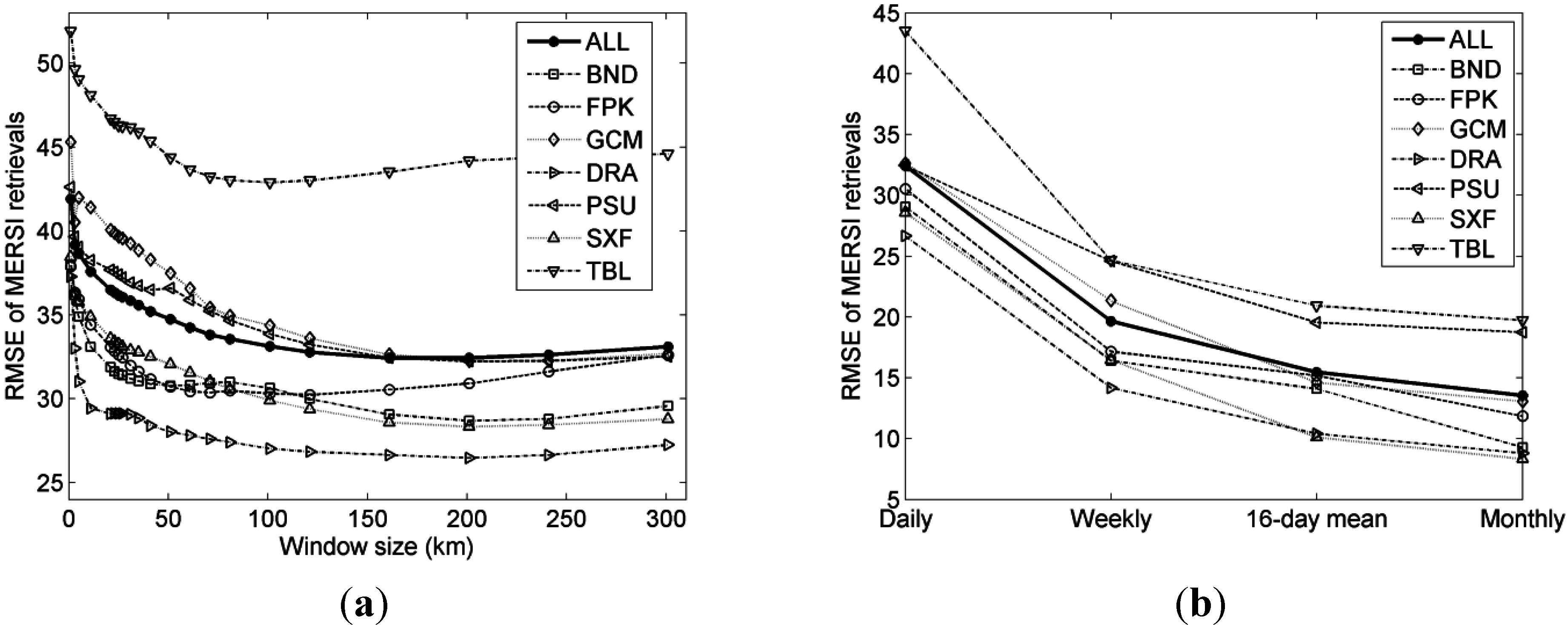
4.1. Scale Effects

Issues of spatial and temporal mismatch will always exists in the validation of daily SSNR data estimated from a single MERSI observation with a spatial resolution of 1 km against field measurements at SUFRAD stations with a footprint of hundreds of meters [18]. Better agreement between radiative fluxes measured and retrieved can be achieved by temporally averaging tower measurements [19] or spatially aggregating satellite data [20]. Here, we investigated how spatial and temporal resolution may affect the retrieval accuracy of SSNR data from the MERSI (Figure 1).

Figure 1. Change of RMSE of estimating daily surface shortwave net radiation (SSNR) from MERSI with spatial (a) and temporal (b) resolutions. Please see Table 3 for the full names of SURFRAD stations.

Figure 1. Change of RMSE of estimating daily surface shortwave net radiation (SSNR) from MERSI with spatial (a) and temporal (b) resolutions. Please see Table 3 for the full names of SURFRAD stations.

The daily SSNR data estimated from the MERSI are first spatially averaged by use of a 1-km–301-km window. Compared with the original retrievals at 1 km, a substantial drop in estimation errors was observed when data were aggregated to slightly coarser resolutions. The drop is much more prominent than that of the MODIS data [8]. For the MODIS results, the errors at some stations even increased slightly when data were initially aggregated to a coarser resolution. With the further increase of window size, we expect to see a rise in estimation errors because of the heterogeneity in surface albedo and cloud coverage. At a 161-km spatial resolution, the MERSI data have the smallest RMSE. This optimal window size to minimize MERSI retrieval errors is much larger than that of MODIS (71 km) [8]. The spatial aggregation might compensate for the uncertainties in geolocation and signal noise on the image. As is mentioned earlier, the limited number of daily overpasses from the polar-orbiting satellite is one of the major sources of uncertainties because intra-daily variations in atmospheric conditions that cannot be well captured by the temporally sparse MERSI observations. In addition to the overall higher data quality of MODIS, the combined MODIS sensors can be another important reason for the difference. Two MODIS sensors result in more overpasses during one day and provide enhanced capability of capturing diurnal variations of atmospheric conditions.

We calculated weekly, 16-day and monthly mean of SSNR from the daily SSNR data retrievals aggregated at a spatial resolution of 161 km, and we assessed how the accuracy of remote sensing of SSNR changes with temporal resolution (Figure 1b). Similarly, averaging in the temporal domain can also reduce the uncertainties in estimating SSNR from the MERSI data. The average accuracy of estimating daily SSNR is ~30 W/m². The error can be reduced to ~20 W/m² for the weekly SSNR and ~15 W/m² for the monthly SSNR. For the monthly data, three of the seven stations—Bondville, Illinois; Desert Rock, Nevada; and Sioux Falls, South Dakota—have RMSEs smaller than 10 W/m².

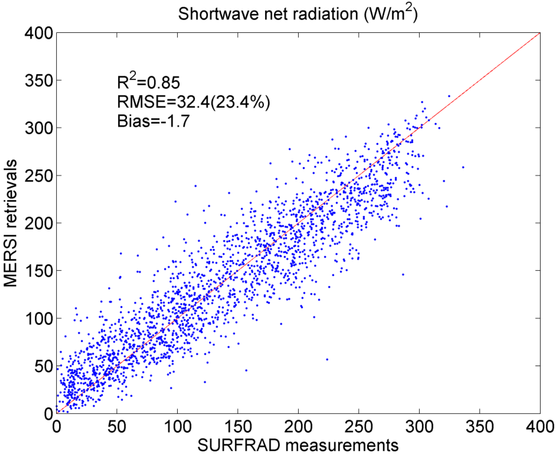
4.2. Validation Results

At its original spatial resolution, the presented approach can retrieve daily SSNR with an RMSE of 41.9 W/m² (30.0%) and a small negative bias of −1.6 W/m² from the MERSI data (Figure 2). This accuracy is comparable to the result of an early study that used MODIS (41.0 W/m²; [17]), where the atmospheric absorption band was not used and the effects of water vapor absorption were corrected with external data of water vapor concentration. The accuracy of the MODIS results has recently been improved to 35.6 W/m² from Aqua, 34.5 W/m² from Terra or 28.7 W/m² from the combined data by Wang et al. [8]. Although the bias from MERSI is smaller than the recent results obtained when using MODIS, the estimation errors from MERSI are approximately 7 W/m² greater than those from a single MODIS sensor.

Figure 2. Scatter plot between daily SSNR measured at SURFRAD stations and retrieved from MERSI at the original spatial resolution.

Figure 2. Scatter plot between daily SSNR measured at SURFRAD stations and retrieved from MERSI at the original spatial resolution.

According to the earlier discussion, appropriate spatial aggregation is able to reduce the errors in estimating daily SSNR from the MERSI data, where intra-daily variations in atmospheric conditions are not considered. The validation results of the MERSI data retrievals aggregated at 161 km are summarized in Table 3 and Figure 3. Compared with the results at the native resolution, the aggregated daily SSNR from the MERSI data sees a reduction of 9.5 W/m² in RMSE. The R² value also improves from 0.76 to 0.85.

Substantial difference exists in validation results across sites (Table 3). Desert Rock, a homogeneous sparsely vegetated site, has the smallest RMSE of 26.6 W/m². The MERSI data have the largest uncertainties of 43.5 W/m² (28.7%) at Boulder, Colorado. Daily SSNR data from the MODIS and CERES data also have the greatest errors at this site [8]. To further investigate the cause of large errors at the site, we examined the in situ data measured at Boulder. Large intra-daily variations in the downward shortwave radiations exist at the site. The variations will lead to an error of 30.7 W/m² and underestimation of 13.3 W/m² if the afternoon measurements of SSNR are used to infer the daily values. The accuracy of estimating daily SSNR from the afternoon measurements at Boulder are ~10 W/m² greater than the average accuracy at the other six sites. Hence, great intra-daily variations of atmospheric conditions at Boulder cause difficultly in accurately estimating daily SSNR from a limited number of satellite observations during the day. This also suggests the importance of a geostationary satellite in monitoring intra-daily dynamics of atmospheric conditions.

Figure 3. Scatter plot between daily SSNR measured at SURFRAD stations and that retrieved from MERSI and aggregated to the spatial resolution of 161 km.

Figure 3. Scatter plot between daily SSNR measured at SURFRAD stations and that retrieved from MERSI and aggregated to the spatial resolution of 161 km.

Table 3. Summary of validation results of daily SSNR retrieved from MERSI and aggregated to 161 km over SUFRAD stations.

Station	Abbreviation	Latitude	Longitude	R2	RMSE (W/m2)	Relative RMSE (%)	Bias (W/m2)
Bondville, IL	BND	40.05	−88.37	0.87	29.1	23.2	1.7
Fort Peck, MT	FPK	48.31	−105.10	0.88	30.5	25.1	−2.9
Goodwin Creek, MS	GCM	34.25	−89.87	0.83	32.6	22.3	4.4
Desert Rock, NV	DRA	36.63	−116.02	0.86	26.6	14.3	−3.6
Penn State, PA	PSU	40.72	−77.93	0.85	32.5	28.4	10.2
Sioux Falls, SD	SXF	43.73	−96.62	0.88	28.6	23.0	−5.0
Boulder, CO	TBL	40.13	−105.24	0.74	43.5	28.7	−15.7
Overall	ALL	-	-	0.85	32.4	23.4	−1.7

Table 3. Summary of validation results of daily SSNR retrieved from MERSI and aggregated to 161 km over SUFRAD stations.

Station	Abbreviation	Latitude	Longitude	R2	RMSE (W/m2)	Relative RMSE (%)	Bias (W/m2)
Bondville, IL	BND	40.05	−88.37	0.87	29.1	23.2	1.7
Fort Peck, MT	FPK	48.31	−105.10	0.88	30.5	25.1	−2.9
Goodwin Creek, MS	GCM	34.25	−89.87	0.83	32.6	22.3	4.4
Desert Rock, NV	DRA	36.63	−116.02	0.86	26.6	14.3	−3.6
Penn State, PA	PSU	40.72	−77.93	0.85	32.5	28.4	10.2
Sioux Falls, SD	SXF	43.73	−96.62	0.88	28.6	23.0	−5.0
Boulder, CO	TBL	40.13	−105.24	0.74	43.5	28.7	−15.7
Overall	ALL	-	-	0.85	32.4	23.4	−1.7

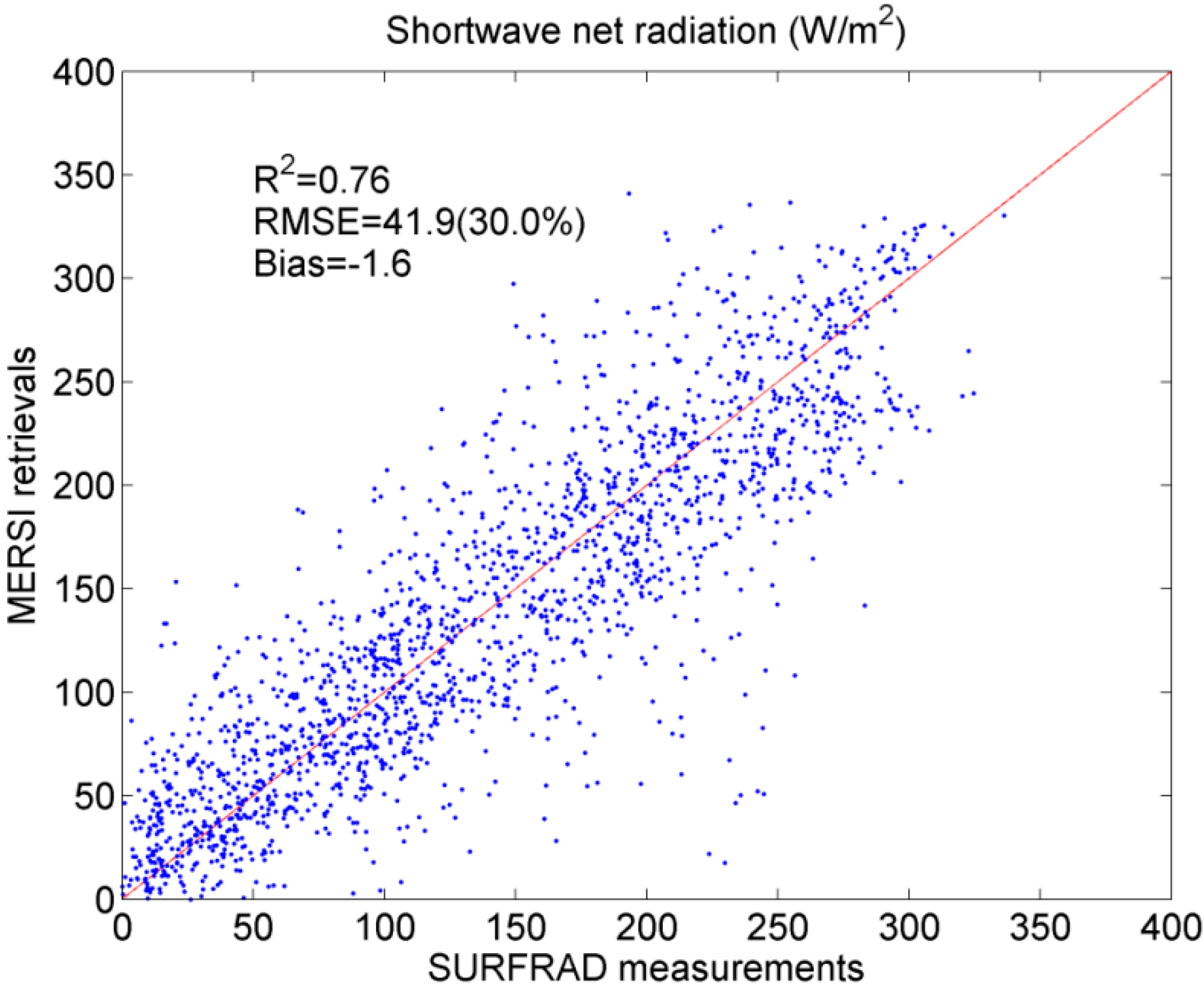
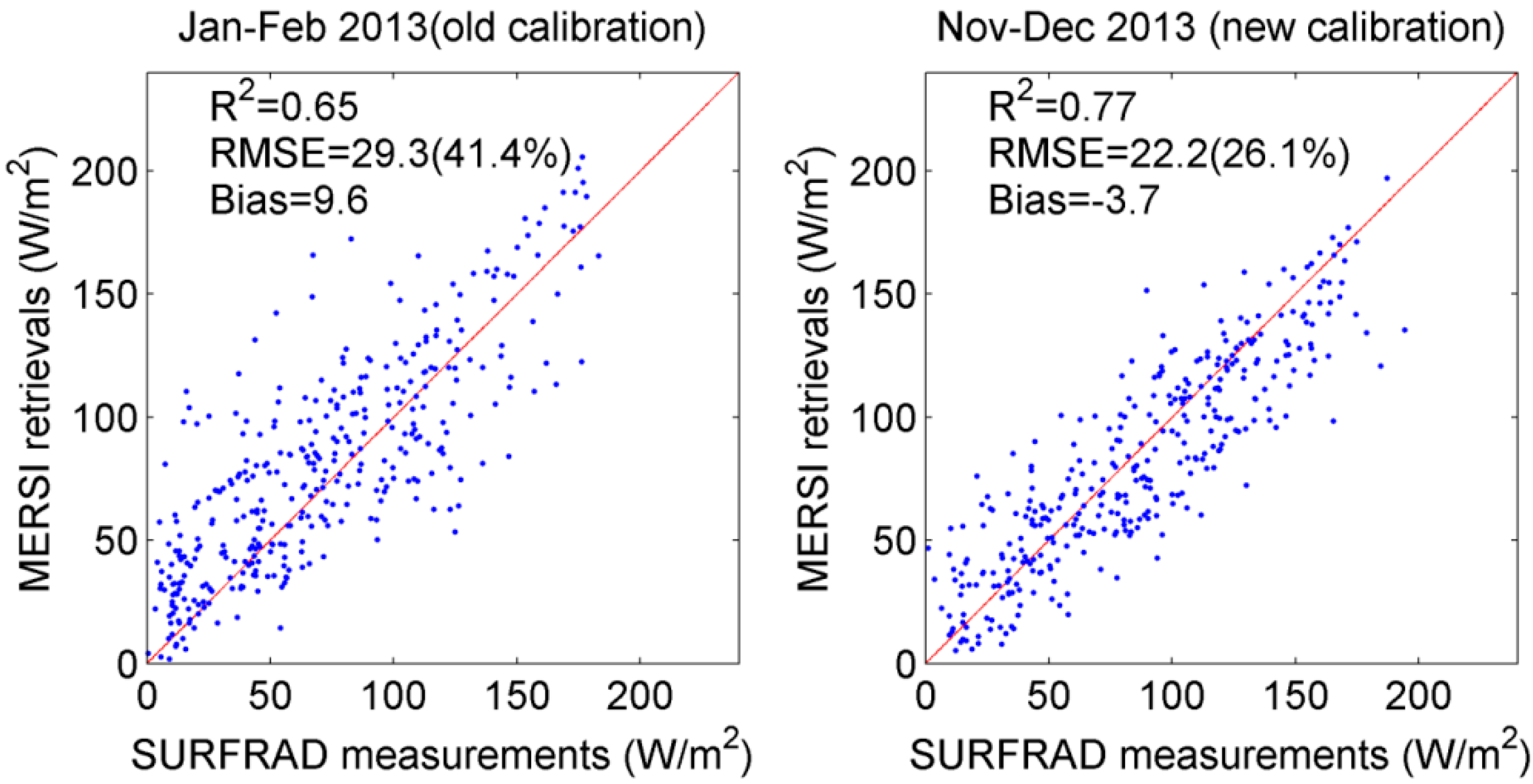
4.3. Impacts of the Updated Radiometric Calibration

During the year 2013, the FY-3B MERSI received a major update to its radiometric calibration. The new daily updated coefficients, based on the empirical degradation equation, have been applied to all of the data acquired after 6 March. To assess the impacts of such a calibration update on the retrieval of high-level products, such as daily SSNR data, we compared data before and after this calibration update. To achieve a fair comparison, we chose data with a similar Sun declination angle and, thus, the trajectory of the solar zenith angle during a day. Results from Day of Year (DOY) 1–64 and from DOY 280–343 were used for comparison, to represent data before and after the update (Figure 4). Clearly, the calibration update has improved the quality of the estimated daily SSNR. Results after the update are better than those before according to all three criteria, higher R², smaller RMSE and bias. The reduction in the RMSE and bias is as high as 6–7 W/m², representing a 9% reduction in relative error. The importance of the stability of sensor calibration for monitoring the trends and long-term environmental changes from space-based observations is well recognized. It is not surprising that the subtle drift in sensor calibration can cause artifacts in trend analysis [21]. Modern optical remote-sensing data have improved substantially in calibration reliability through the use of onboard calibration devices [22] or vicarious calibration techniques [23]. The MERSI data generally have a lower requirement in calibration accuracy (7%; [16]) than the MODIS data (2% for reflectance and 5% for radiance; [24]). The shorter wavelength bands of the MERSI have experienced serious sensor degradation. According to an independent study, the total degradation rate of Band 8 (412 nm) within three years is near 40% [25]. Its two shortwave infrared channels (Band 6, 1.64 µm, and Band 7, 2.13 µm) started to operate in anomalous status shortly after the launch because of a malfunction of the passive radiant cooler [16]. As a result, SSNR data retrieved from MERSI generally has worse quality than that from MODIS. Nevertheless, the recent calibration update improved the radiometric accuracy of the MERSI data and, thus, the quality of the SSNR data retrievals.

Figure 4. Comparison of validation results of daily SSNR from MERSI before and after the calibration update on 6 March 2013.

Figure 4. Comparison of validation results of daily SSNR from MERSI before and after the calibration update on 6 March 2013.

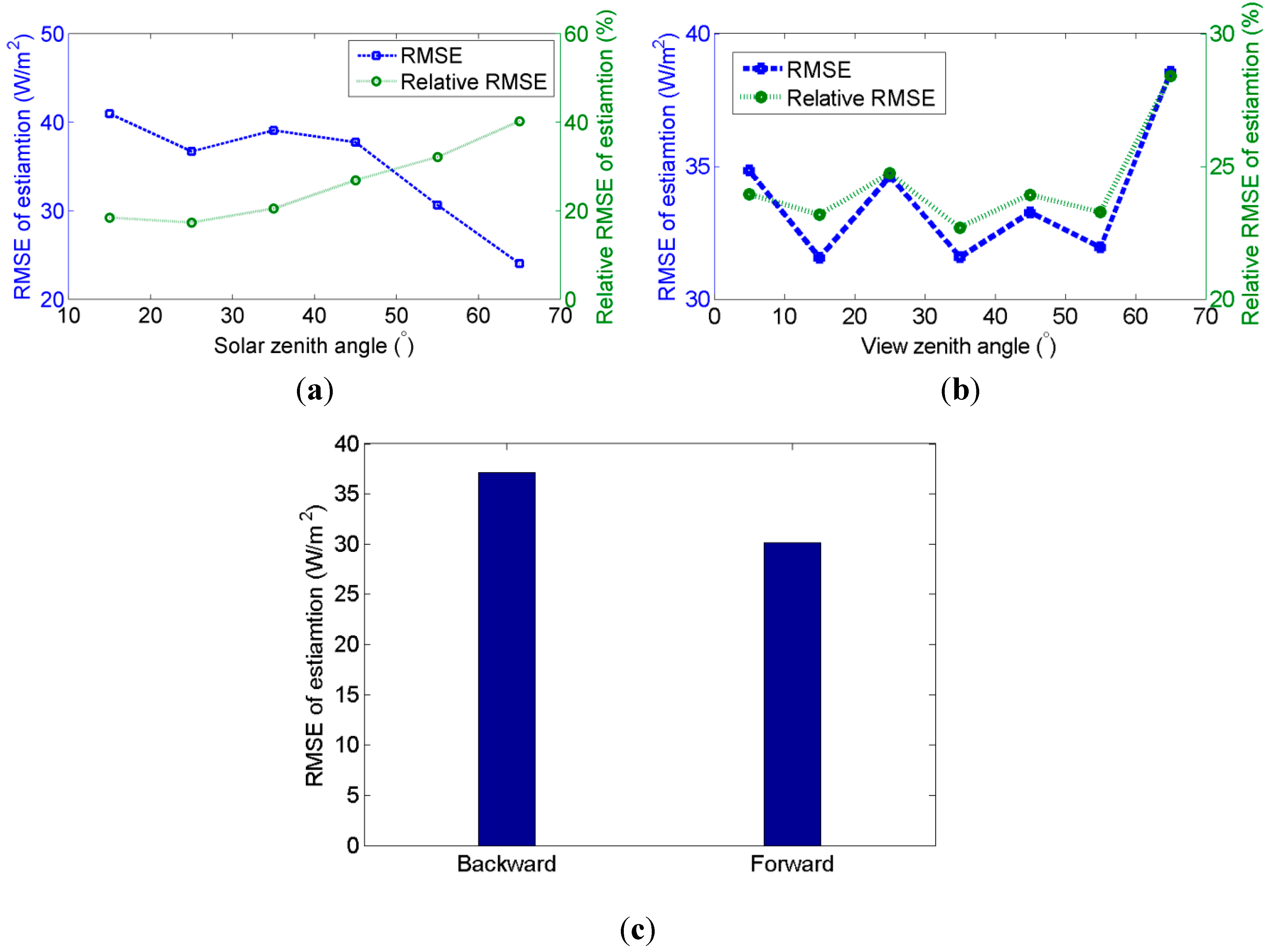
4.4. Dependency on View Geometry

Wide-swath sensors have the advantage of covering larger areas with one overpass and achieving higher revisit frequency. Even so, geostationary satellites are needed to provide sufficient revisit frequency for the low and mid-latitude area. On the other hand, a large range of view zenith angles may also cause variations in data retrieval accuracy because of a difference in atmospheric interaction and surface BRDF. We examined the dependency of retrieval errors on various parameters of view geometry, by binning the validation results according to their solar zenith angle (SZA), view zenith angle (VZA) and relative azimuth angle (RAA) (Figure 5). The absolute error of estimating daily SSNR gradually decreases from 40 W/m² at a SZA of 15° to 25 W/m² at a SZA of 65°. However, it should be noted that relative errors of retrieving SSNR may not necessarily be low when the Sun is low. The SZA for the overpass time mainly changes with the season for the MERSI circling on a Sun-synchronous orbit. A smaller SZA generally means a smaller amount of daily downward shortwave radiation. Thus, the relative RMSE for daily SSNR data retrieval increases from 30% to 40 % when the SZA changes from 15° to 65°. Unlike the SZA, the VZA has little impact on both the absolute and relative RMSE. The estimation errors stay relatively stable when the VZA is smaller than 60°, varying from 22% to 25%. However, for very oblique observations (VZA = 65°), the data retrieval errors increase dramatically, to as large as 38 W/m² (28%). Several factors may explain the large uncertainties resulting from a large VZA. High oblique observations mean little information on the surface, where SSNR is largely regulated by surface albedo. Besides, the footprint of the sensor also increases dramatically with the VZA. RAA also affects the retrieval accuracy of daily SSNR data. We divided the data into two groups according to whether the value of RAA is greater than 90°. When RAA is smaller than 90°, the electromagnetic signature is scatted backward from the surface and then received by the sensor; these data are called backward observations. Backward observations tend to generate 7 W/m² or larger errors than forward observations. This result is mainly related to the hot-spot effect. The signature from backward scattering, and, especially, on the principal plane around the hot-spot directions, has greater variations and is more difficult to model with high accuracy.

Figure 5. Dependency of retrieval accuracy of daily SSNR on view geometry: (a) solar zenith angle, (b) view zenith angle and (c) relative azimuth angle (backward and forward direction).

Figure 5. Dependency of retrieval accuracy of daily SSNR on view geometry: (a) solar zenith angle, (b) view zenith angle and (c) relative azimuth angle (backward and forward direction).

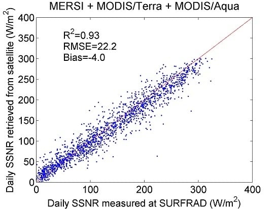
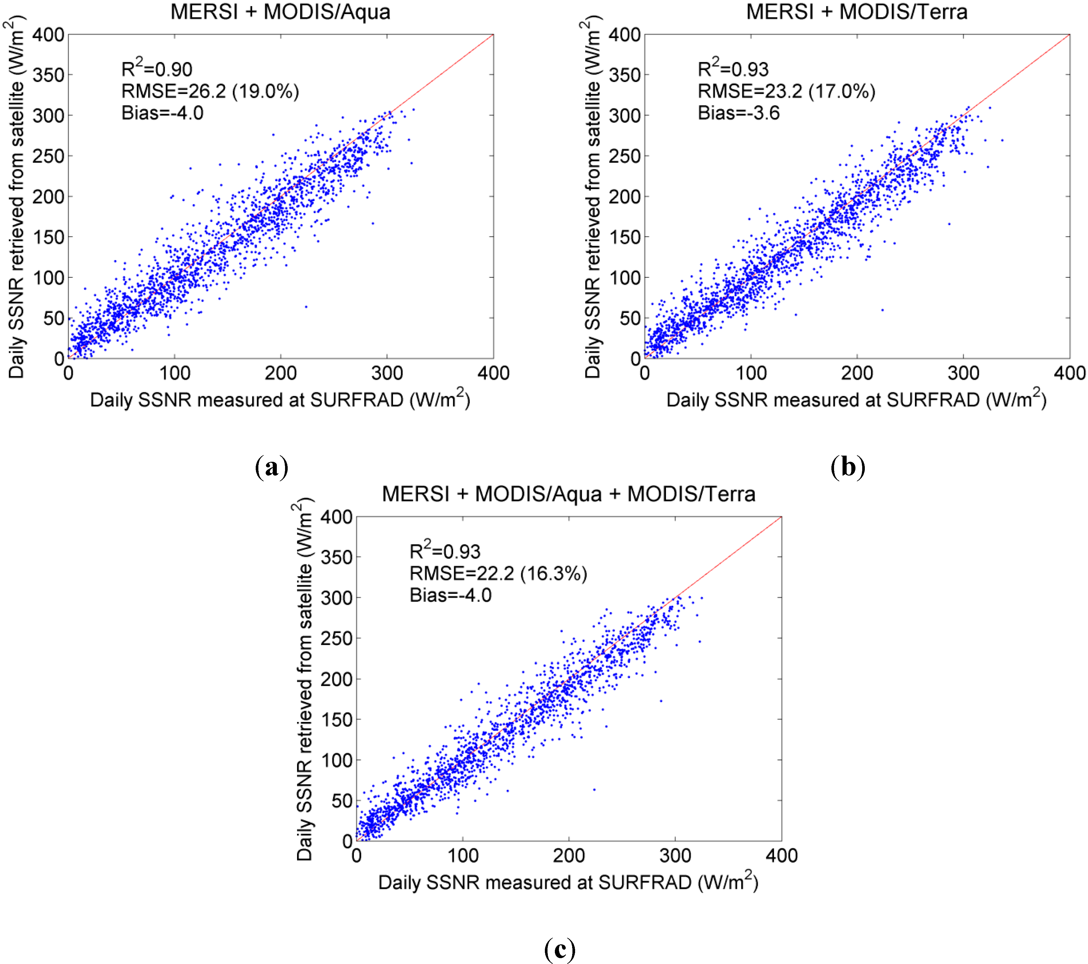
4.5. Combining with MODIS Data

The MODIS data were combined with the MERSI data to evaluate how timing and counts of observations affect the accuracy of estimating daily SSNR. When multiple retrievals from various sensors are available, the simple mean of all of the SSNR retrievals for one day is used as the combined SSNR for that day. We assessed several different data-fusion strategies by adding a single MODIS sensor onboard either Terra or Aqua or adding both MODIS sensors (Figure 6). With additional MODIS data, the accuracy of daily SSNR data retrievals from the MERSI can be improved. By combining MERSI data with the morning MODIS Terra data, the RMSE was reduced from 32.4 to 23.2 W/m². This change also represents a reduction of 2.7 W/m² from the results with only the MODIS/Terra data. The accuracy of combining MODIS/Terra data and the MERSI data is very similar to that of combining two MODIS sensors (23.1 W/m²; [8]). Daily SSNR from the combined two afternoon datasets (MERSI and MODIS Aqua) has an RMSE of 26.2 W/m². Compared with the results from the MERSI data only, this value represents a drop in the RMSE of 6.2 W/m². However, the improvement is only marginal when compared with results from MODIS/Aqua only. By use of data from all three sensors, daily SSNR can be estimated with an RMSE of 22.2 W/m² and a bias of −4.0 W/m², reflecting a reduction of 0.9 W/m² in the RMSE and 2.7 W/m² in bias compared with the results from the twin MODIS sensors.

Figure 6. Validation results of daily SSNR by combining MERSI with MODIS data (a) from MODIS/Aqua only, (b) from MODIS/Terra only and (c) from twin MODIS sensors.

Figure 6. Validation results of daily SSNR by combining MERSI with MODIS data (a) from MODIS/Aqua only, (b) from MODIS/Terra only and (c) from twin MODIS sensors.

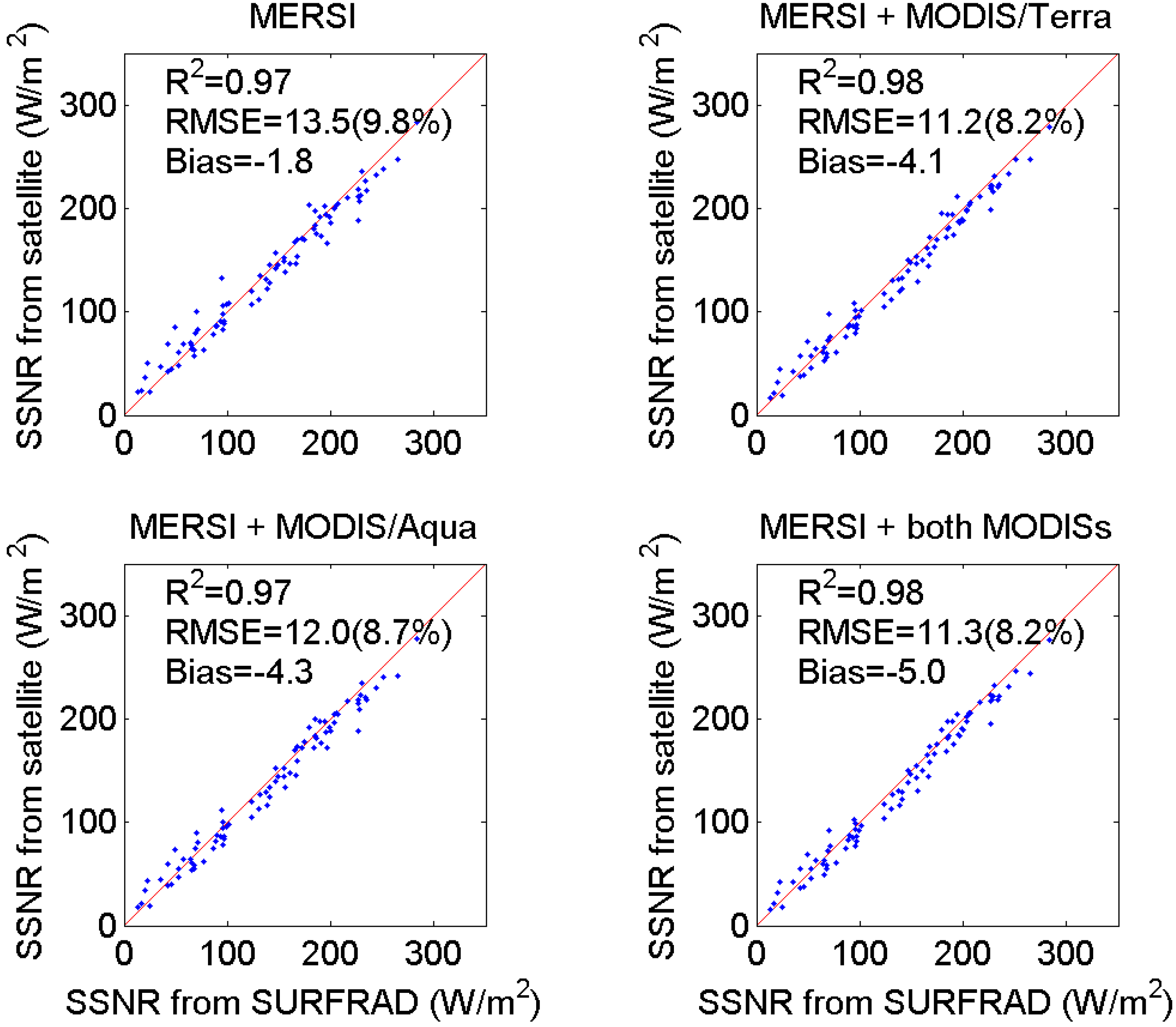
4.6. Monthly Estimates

Many climate studies may need SSNR data of coarser temporal resolutions. The MERSI results of daily SSNR were temporally aggregated to the monthly step and validated against field measurements of monthly SSNR (Figure 7). The comparison results show that a single MERSI sensor can estimate monthly SSNR with an RMSE of 13.5 W/m² (9.8%) and a bias of −1.8 W/m². Both values are smaller than those of the CERES product (14.0 and 7.3 W/m², respectively; [8]). The accuracy of the MERSI retrievals is also close to that of the combined MODIS data (11.6 and −7.1 W/m², respectively; [8]). Similar to what we have done with daily SSNR, we combined the MERSI results of the monthly SSNR with the MODIS results to study the impacts of data fusion on retrievals of monthly SSNR data. The additional MODIS data do improve the quality of monthly SSNR for all scenarios, but the reduction in the RMSE here is not as significant as that for daily SSNR. Not surprisingly, a combination of morning MODIS data will have better results than the use of afternoon MODIS data. The combined MODIS/Terra and MERSI data generate values of monthly SSNR slightly better than the combined two MODIS sensors, mainly because of the reduction in bias when combining two different sensors.

Figure 7. Scatter plot between monthly SSNR measured at SURFRAD stations and retrieved from satellite data and aggregated to a spatial resolution of 161 km.

Figure 7. Scatter plot between monthly SSNR measured at SURFRAD stations and retrieved from satellite data and aggregated to a spatial resolution of 161 km.

5. Conclusions

The FY-3 series is China’s second generation of polar-orbiting meteorological satellites. MERSI, as one of FY-3’s key payloads, succeeds the previous generation of radiometer, the Visible and Infra-Red Radiometer (VIRR), with more spectral channels, higher spatial resolution and improved radiometric calibration. The MODIS-like MERSI data can provide valuable information for various terrestrial, atmospheric and oceanographic research projects at the continental to global scales. Datasets of several variables have been routinely generated from the MERSI data by the National Satellite and Meteorological Center of China. However, there are no MERSI products on surface radiative fluxes. In this study, we presented a direct-estimation algorithm to produce daily SSNR data from MERSI using the MERSI L1b TOA-reflectance and cloud-detection products as inputs. To the best of our knowledge, this paper is the first study to use China’s MERSI data to retrieve SSNR. Several critical issues on remote sensing of SSNR were investigated in the study, including scale effects in validating MERSI SSNR, impacts of MERSI’s calibration update on estimating SSNR and the dependency of the retrieval accuracy of SSNR on view geometry. In addition, the data from twin MODIS sensors were incorporated to assess how the timing and count of observations affect the retrieval of daily SSNR data.

One-year data over seven SURFRAD stations were used to validate SSNR retrieved from MERSI data. Because of the limited number of overpasses each day from the polar-orbiting satellites, MERSI data cannot capture the intra-daily variations in atmospheric conditions, such as aerosol loadings, cloud coverage and water vapor concentrations. These variations will results in uncertainties in retrieving daily SSNR from MERSI data. At the original resolution, daily SSNR retrieved from MERSI data has an RMSE of 41.9 W/m² and a bias of −1.6 W/m². Spatially averaging can largely reduce the scattering. Aggregated at 161 km, the RMSE of MERSI retrievals becomes 32.4 W/m², reflecting a decrease of 9.5 W/m². Similarly, temporal aggregation is also able to reduce the uncertainties of retrieving SSNR. At the monthly scale, the RMSE of retrieving SSNR was significantly reduced to 13.5 W/m².

Compared with results from MODIS, the accuracy of daily SSNR from MERSI is considerably worse. The RMSE of the MERSI results is 6–7 W/m² greater than that from a single MODIS sensor. The difference in spectral configurations between the two sensors can explain little of such a difference in errors, because the theoretical RMSEs of the regression models from the simulated training data show little difference between the two sensors. The quality of radiometric calibration is a key factor affecting the accuracy of the derived high-level products of SSNR. Our comparison suggested that the new calibration approach for MERSI, which is based on the empirical degradation formula, can improve the accuracy of daily SSNR by 7 W/m². The continuous monitoring of sensor degradation and periodic updates of calibration parameters are essential to assure the quality of high-level products retrieved from the MERSI data.

The optimal window size of spatial aggregation to minimize errors for the MERSI data retrievals is more than twice as large as that of the MODIS data. In addition to image noise, geolocation errors of the MERSI data can explain why a larger window is needed to smooth out the retrieval uncertainties. A global positioning system (GPS), with the assistance of a high-precision orbit model, was used to calculate the locations of the FY-3 satellites [26]. Techniques, such as rotation offsetting of the K-mirror, were used to improve the accuracy of the geometric registration of the MERSI data [27]. Nevertheless, an independent analysis shows that the geometric error between the MERSI and the MODIS data is 2–3 pixels [28]. Although the MODIS data have achieved geometric accuracy at the subpixel level, additional efforts are needed to improve georegistration of the MERSI data.

We demonstrated the importance of multiple observations per day in estimating daily SSNR. By combining the morning Terra MODIS data with the afternoon FY-3B MERSI data, we can reduce the estimated errors by 9.2 W/m² and achieve accuracy similar to that from the combined morning and afternoon MODIS data. The number of observations per day has smaller impacts on errors in estimating monthly SSNR than in estimating daily SSNR. With the launch of FY-3C on 23 September 2013, a total of three MERSI sensors are currently in operation. Another five FY-3 satellites, including two morning satellites and three afternoon satellites, are currently at the planning stage. The future network of FY-3 satellites is expected to generate better global products of daily SSNR and to improve our understanding of the surface radiation budget.

References

1. Liang, S.; Wang, K.; Zhang, X.; Wild, M. Review on estimation of land surface radiation and energy budgets from ground measurement, remote sensing and model simulations. IEEE J. Sel. Top. Appl. Earth Obs. Remote Sens. 2010, 3, 225–240. [Google Scholar] [CrossRef]
2. Liang, S.; Zhang, X.; He, T.; Cheng, J.; Wang, D. Remote sensing of earth surface radiation budget. In Remote Sensing of Land Surface Turbulent Fluxes and Soil Surface Moisture Content: State of the Art; Petropoulos, G.P., Ed.; CRC Press: Boca Raton, FL, USA, 2013; pp. 125–165. [Google Scholar]
3. Jiang, B.; Zhang, Y.; Liang, S.; Zhang, X.; Xiao, Z. Surface daytime net radiation estimation using artificial neural networks. Remote Sens. 2014, 6, 11031–11050. [Google Scholar] [CrossRef]
4. Bisht, G.; Bras, R.L. Estimation of net radiation from the MODIS data under all sky conditions: Southern great plains case study. Remote Sens. Environ. 2010, 114, 1522–1534. [Google Scholar] [CrossRef]
5. Wang, D.; Liang, S. Mapping high-resolution surface shortwave net radiation from Landsat data. IEEE Geosci. Remote Sens. Lett. 2014, 11, 459–463. [Google Scholar] [CrossRef]
6. Tang, B.H.; Li, Z.L.; Zhang, R.H. A direct method for estimating net surface shortwave radiation from MODIS data. Remote Sens. Environ. 2006, 103, 115–126. [Google Scholar] [CrossRef]
7. He, T.; Liang, S.; Wang, D.; Shi, Q.; Goulden, M.L. Estimation of high-resolution land surface net shortwave radiation from AVIRIS data: Algorithm development and preliminary results. Remote Sens. Environ. 2014. [Google Scholar] [CrossRef]
8. Wang, D.; Liang, S.; He, T.; Shi, Q. Estimation of daily surface shortwave net radiation from the combined MODIS data. IEEE Trans. Geosci. Remote Sens. 2015, in press. [Google Scholar]
9. Sun, L.; Guo, M.; Zhu, J.; Hu, X.; Song, Q. FY-3A/MERSI, ocean color algorithm, products and demonstrative applications. Acta Oceanol. Sin. 2013, 32, 75–81. [Google Scholar] [CrossRef]
10. Yang, Z.; Lu, N.; Shi, J.; Zhang, P.; Dong, C.; Yang, J. Overview of FY-3 payload and ground application system. IEEE Trans. Geosci. Remote Sens. 2012, 50, 4846–4853. [Google Scholar] [CrossRef]
11. Hu, X.; Liu, J.; Sun, L.; Rong, Z.; Li, Y.; Zhang, Y.; Zheng, Z.; Wu, R.; Zhang, L.; Gu, X. Characterization of CRCS dunhuang test site and vicarious calibration utilization for Fengyun (FY) series sensors. Can. J. Remote Sens. 2010, 36, 566–582. [Google Scholar] [CrossRef]
12. Sun, L.; Hu, X.; Guo, M.; Xu, N. Multisite calibration tracking for FY-3A MERSI solar bands. IEEE Trans. Geosci. Remote Sens. 2012, 50, 4929–4942. [Google Scholar] [CrossRef]
13. Kotchenova, S.Y.; Vermote, E.F.; Levy, R.; Lyapustin, A. Radiative transfer codes for atmospheric correction and aerosol retrieval: Intercomparison study. Appl. Opt. 2008, 47, 2215–2226. [Google Scholar] [CrossRef] [PubMed]
14. Schaaf, C.B.; Gao, F.; Strahler, A.H.; Lucht, W.; Li, X.W.; Tsang, T.; Strugnell, N.C.; Zhang, X.Y.; Jin, Y.F.; Muller, J.P.; et al. First operational BRDF, albedo nadir reflectance products from MODIS. Remote Sens. Environ. 2002, 83, 135–148. [Google Scholar] [CrossRef]
15. Kaufman, Y.J.; Tanre, D.; Remer, L.A.; Vermote, E.F.; Chu, A.; Holben, B.N. Operational remote sensing of tropospheric aerosol over land from EOS moderate resolution imaging spectroradiometer. J. Geophys. Res. Atmos. 1997, 102, 17051–17067. [Google Scholar] [CrossRef]
16. Sun, L.; Hu, X.; Xu, N.; Liu, J.; Zhang, L.; Rong, Z. Postlaunch calibration of Fengyun-3B MERSI reflective solar bands. IEEE Trans. Geosci. Remote Sens. 2013, 51, 1383–1392. [Google Scholar] [CrossRef]
17. Kim, H.Y.; Liang, S. Development of a hybrid method for estimating land surface shortwave net radiation from MODIS data. Remote Sens. Environ. 2010, 114, 2393–2402. [Google Scholar] [CrossRef]
18. Román, M.O.; Schaaf, C.B.; Woodcock, C.E.; Strahler, A.H.; Yang, X.; Braswell, R.H.; Curtis, P.S.; Davis, K.J.; Dragoni, D.; Goulden, M.L.; et al. The MODIS (collection v005) BRDF/albedo product: Assessment of spatial representativeness over forested landscapes. Remote Sens. Environ. 2009, 113, 2476–2498. [Google Scholar] [CrossRef]
19. Gupta, S.K.; Kratz, D.P.; Wilber, A.C.; Nguyen, L.C. Validation of parameterized algorithms used to derive TRMM-CERES surface radiative fluxes. J. Atmos. Ocean. Technol. 2004, 21, 742–752. [Google Scholar] [CrossRef]
20. Wang, D.; Liang, S.; Liu, R.; Zheng, T. Estimation of daily-integrated PAR from sparse satellite observations: Comparison of temporal scaling methods. Int. J. Remote Sens. 2010, 31, 1661–1677. [Google Scholar] [CrossRef]
21. Wang, D.D.; Morton, D.; Masek, J.; Wu, A.S.; Nagol, J.; Xiong, X.X.; Levy, R.; Vermote, E.; Wolfe, R. Impact of sensor degradation on the MODIS NDVI time series. Remote Sens. Environ. 2012, 119, 55–61. [Google Scholar] [CrossRef]
22. Xiong, X.X.; Sun, J.Q.; Xie, X.B.; Barnes, W.L.; Salomonson, V.V. On-orbit calibration and performance of Aqua MODIS reflective solar bands. IEEE Trans. Geosci. Remote Sens. 2010, 48, 535–546. [Google Scholar] [CrossRef]
23. Wu, A.S.; Xiong, X.X.; Doelling, D.R.; Morstad, D.; Angal, A.; Bhatt, R. Characterization of terra and aqua MODIS VIS, NIR, and SWIR spectral bands’ calibration stability. IEEE Trans. Geosci. Remote Sens. 2013, 51, 4330–4338. [Google Scholar] [CrossRef]
24. Xiong, X.; Barnes, W.; Chiang, K.; Erives, H.; Che, N.; Sun, J.; Isaacman, A.; Salomonson, V. Status of Aqua MODIS on-orbit calibration and characterization. Proc. SPIE 2013. [Google Scholar] [CrossRef]
25. Kim, W.; Cao, C.; Liang, S. Assessment of radiometric degradation of Fy-3A MERSI reflective solar bands using TOA reflectance of pseudoinvariant calibration sites. IEEE Geosci. Remote Sens. Lett. 2014, 11, 793–797. [Google Scholar] [CrossRef]
26. Guan, M.; Wu, R. Geolocation approach for Fy-3A MERSI remote sesning image. J. Appl. Meteorol. Sci. 2012, 23, 534–542. (in Chinese). [Google Scholar]
27. Guan, M.; Guo, Q. Offsetting image rotation system in Fy-3 MERSI’s geolocation. J. Appl. Meteorol. Sci. 2008, 19, 420–427. (in Chinese). [Google Scholar]
28. Zhao, Y.; Shan, X.; Tang, P. Spatial consitency analysis and relative geometric correction of low spatial resolution mulit-source remote sensing data. Remote Sens. Tech. Appl. 2014, 29, 155–163. (in Chinese). [Google Scholar]