
Application of Multispectral Sensors Carried on Unmanned Aerial Vehicle (UAV) to Trophic State Mapping of Small Reservoirs: A Case Study of Tain-Pu Reservoir in Kinmen, Taiwan

Abstract
:
1. Introduction
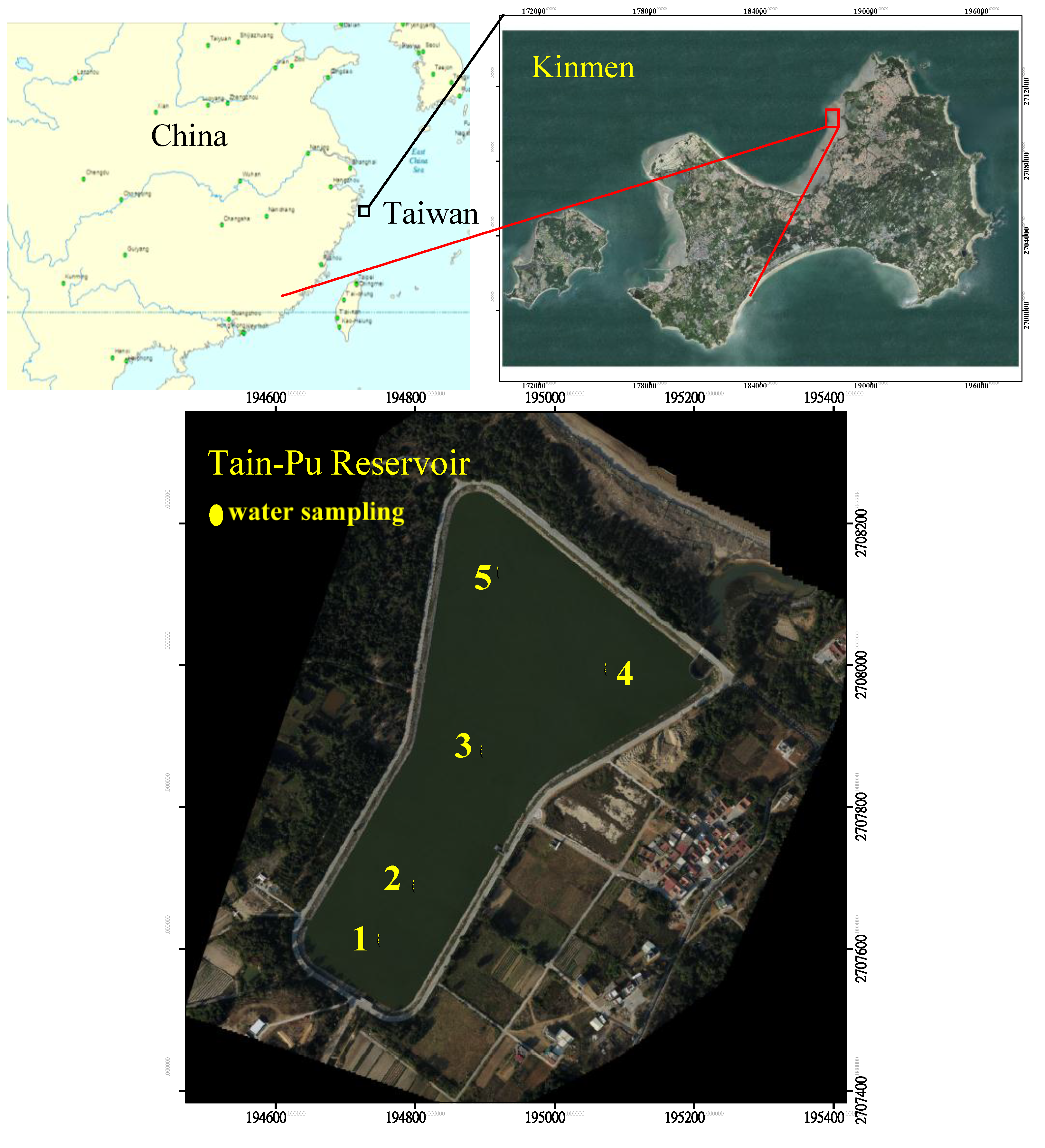
2. Study Site


| Parameter | Climatic Season | ||||
|---|---|---|---|---|---|
| Spring | Summer | Fall | Winter | ||
| SD (m) | Range | 0.1–0.6 | 0.2–0.8 | 0.2–0.5 | 0.1–1.2 |
| Mean | 0.4 | 0.4 | 0.4 | 0.5 | |
| Std. | 0.2 | 0.2 | 0.1 | 0.3 | |
| Chl-a (μg·L−1) | Range | 24.5–143.0 | 23.2–124.0 | 2.4–191.0 | 12.2–158.0 |
| Mean | 59.0 | 69.9 | 75.9 | 58.0 | |
| Std. | 35.8 | 26.4 | 61.6 | 40.4 | |
| TP (μg·L−1) | Range | 25.0–126.0 | 17.9–139.0 | 18.0–177.0 | 42.0–121.0 |
| Mean | 57.6 | 79.9 | 79.9 | 76.6 | |
| Std. | 25.9 | 37.4 | 45.2 | 29.0 | |
| SD | Chl-a | TP | ||
|---|---|---|---|---|
| SD | r | 1 | −0.434 ** | −0.259 |
| Chl-a | r | −0.434 ** | 1 | 0.254 |
| TP | r | −0.259 | 0.254 | 1 |
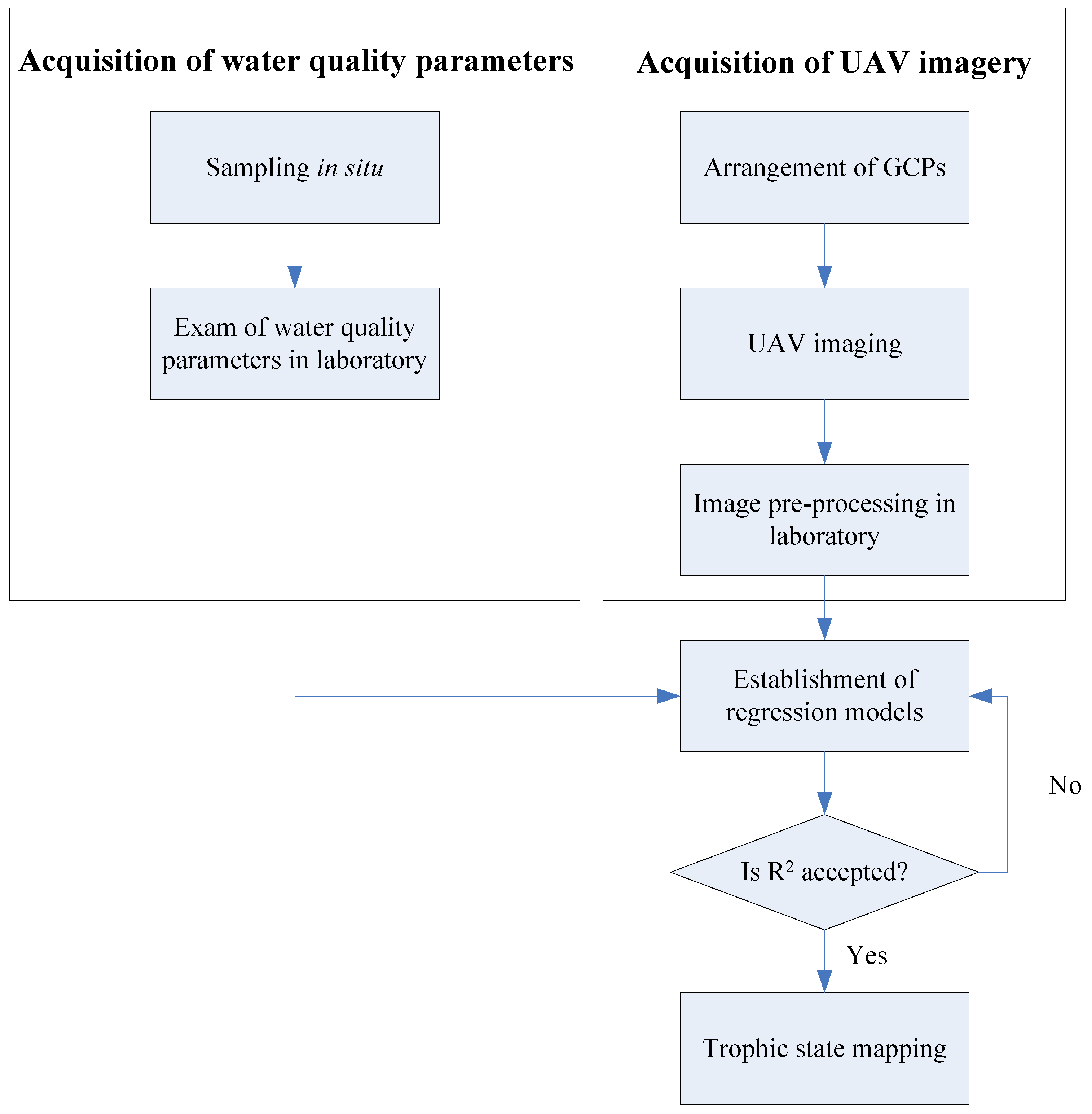
3. Methodology

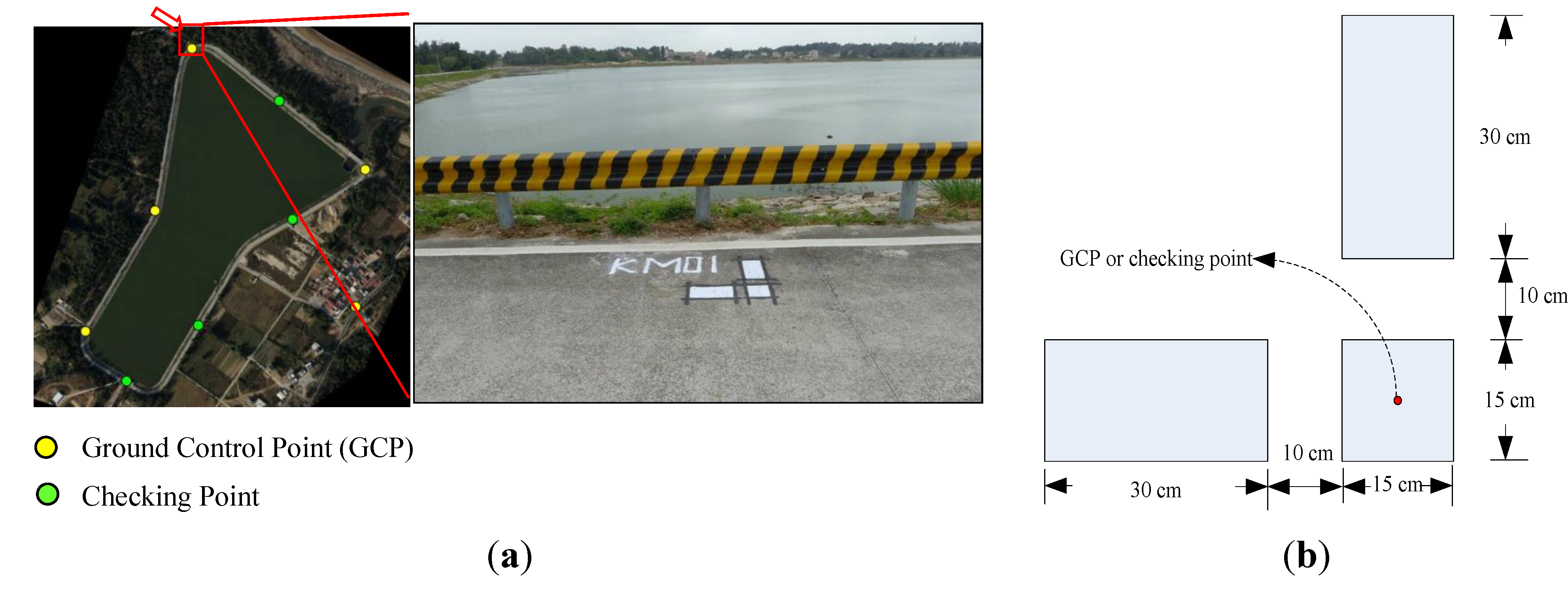
3.1. Measurement In Situ and Water Quality Exam
| No. of Sampling Point | Water Quality Parameter | Sampling Coordinate (System Name: GCS_TWD_1997) | |||
|---|---|---|---|---|---|
| SD (m) | Chl-a (μg·L−1) | TP (μg·L−1) | E (m) | N (m) | |
| 1 | 1.8 | 173.0 | 105.0 | 194,750.14 | 2,707,614.72 |
| 2 | 1.6 | 185.0 | 113.0 | 194,800.16 | 2,707,690.52 |
| 3 | 2.0 | 172.0 | 108.0 | 194,897.61 | 2,707,880.43 |
| 4 | 1.5 | 156.0 | 99.0 | 195,075.60 | 2,707,996.12 |
| 5 | 1.7 | 177.0 | 108.0 | 194,921.69 | 2,708,132.85 |
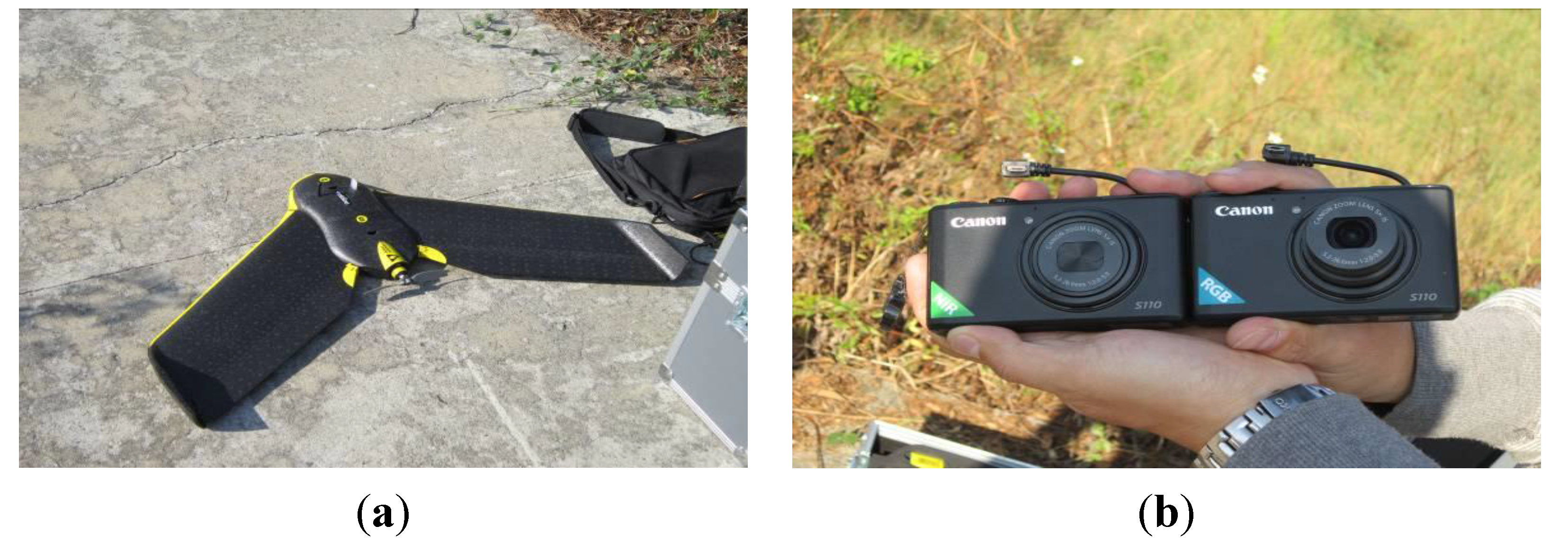
3.2. UAV Multispectral Image Data

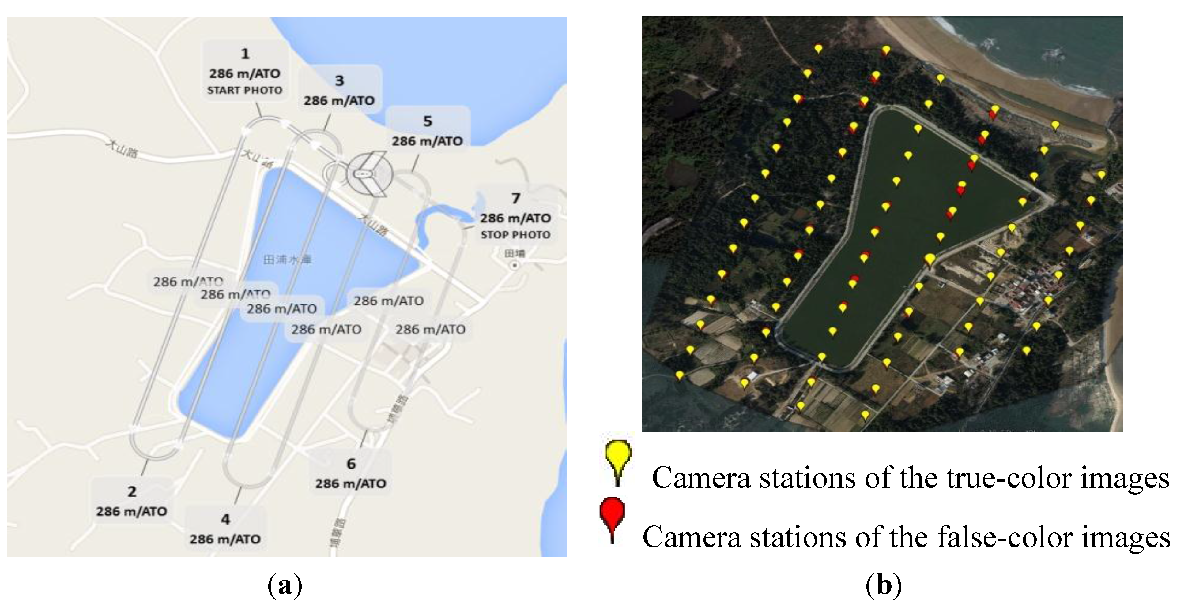
3.3. UAV Imaging


3.4. Image Pre-Processing
3.5. Establishment of Regression Models
3.6. Trophic State Mapping
4. Results of Regression Model Establishment and Trophic State Mapping
4.1. Establishment of Regression Models by the Average Method
| n | Y = Chl-a, X = NIR/R | Y = TP, X = NIR/R | ||||
|---|---|---|---|---|---|---|
| r | r2 | P value | r | r2 | P value | |
| 5 | 0.405 | 0.164 | 0.499 | 0.573 | 0.328 | 0.313 |
| 9 | 0.253 | 0.064 | 0.681 | 0.481 | 0.231 | 0.412 |
| 19 | 0.513 | 0.263 | 0.377 | 0.610 | 0.372 | 0.275 |
| 49 | 0.487 | 0.237 | 0.405 | 0.573 | 0.328 | 0.312 |
| 99 | 0.768 | 0.590 | 0.129 | 0.698 | 0.487 | 0.190 |
| n | Y = SD, X = NIR/R | Y = SD, X = R/B | Y = SD, X = NIR/B | ||||||
|---|---|---|---|---|---|---|---|---|---|
| r | r2 | P value | r | r2 | P value | r | r2 | P value | |
| 5 | 0.759 | 0.576 | 0.137 | −0.445 | 0.198 | 0.452 | −0.218 | 0.048 | 0.725 |
| 9 | 0.423 | 0.179 | 0.478 | −0.419 | 0.176 | 0.482 | −0.405 | 0.164 | 0.498 |
| 19 | 0.245 | 0.060 | 0.692 | −0.334 | 0.112 | 0.582 | −0.275 | 0.076 | 0.655 |
| 49 | 0.222 | 0.049 | 0.720 | −0.338 | 0.114 | 0.579 | −0.318 | 0.101 | 0.602 |
| 99 | −0.015 | 0.000 | 0.980 | −0.243 | 0.059 | 0.694 | −0.222 | 0.049 | 0.719 |
4.2. Establishment of Regression Models by the MPP Method
| X | Y | Correlation Coefficient | Regression Parameters | |||
|---|---|---|---|---|---|---|
| r | r2 | P value | a | b | ||
| NIR/R | Chl-a | 1.000 ** | 1.000 | 0.000 | 1.0814 | 5.0176 |
| TP | 0.999 ** | 0.997 | 0.000 | 0.7118 | 4.5720 | |
| SD | −0.982 ** | 0.963 | 0.003 | −4.0138 | 1.1759 | |
| NIR/B | SD | −0.999 ** | 0.998 | 0.000 | −2.0054 | 0.6414 |
| R/B | SD | −0.823 | 0.677 | 0.087 | −1.7424 | 0.3562 |
| Regression Model | Pij(m) | |||||||||
|---|---|---|---|---|---|---|---|---|---|---|
| m = 1 | m = 2 | m = 3 | m = 4 | m = 5 | ||||||
| i | j | i | j | i | j | i | j | i | j | |
| ln(Chl-a) = 1.0814ln(NIR/R) + 5.0176 (NIR = 34, R = 30, if m = 1) (NIR = 35, R = 29, if m = 2) (NIR = 35, R = 31, if m = 3) (NIR = 34, R = 33, if m = 4) (NIR = 37, R =32, if m = 5) | 1 2 3 | 3 2 3 | 2 | 4 | 5 | 5 | 4 5 | 2 2 | 4 5 | 5 3 |
| ln(TP) = 0.7118ln(NIR/R) + 4.5720 (NIR = 35, R = 31, if m = 1) (NIR = 36, R = 29, if m = 2) (NIR = 35, R = 30, if m = 3) (NIR = 34, R = 33, if m = 4) (NIR = 35, R = 30, if m = 5) | 1 4 4 4 4 | 1 1 2 3 4 | 3 | 3 | 1 | 1 | 4 5 | 2 2 | 2 | 2 |
| 2 | 1 | |||||||||
| 2 | 5 | |||||||||
| 3 | 1 | |||||||||
| 3 | 2 | |||||||||
| 3 | 4 | |||||||||
| 4 | 1 | |||||||||
| 4 | 2 | |||||||||
| 4 | 3 | |||||||||
| 4 | 4 | |||||||||
| 5 | 1 | |||||||||
| 5 | 2 | |||||||||
| 5 | 4 | |||||||||
| ln(SD) = −2.0054ln(NIR/B) + 0.6414 (NIR = 35, B = 34, if m = 1) (NIR = 36, B = 33, if m = 2) (NIR = 35, B = 36, if m = 3) (NIR = 37, B = 33, if m = 4) (NIR = 36, B = 34, if m = 5) | 4 | 4 | 3 | 3 | 2 5 | 5 5 | 1 | 2 | 5 | 2 |
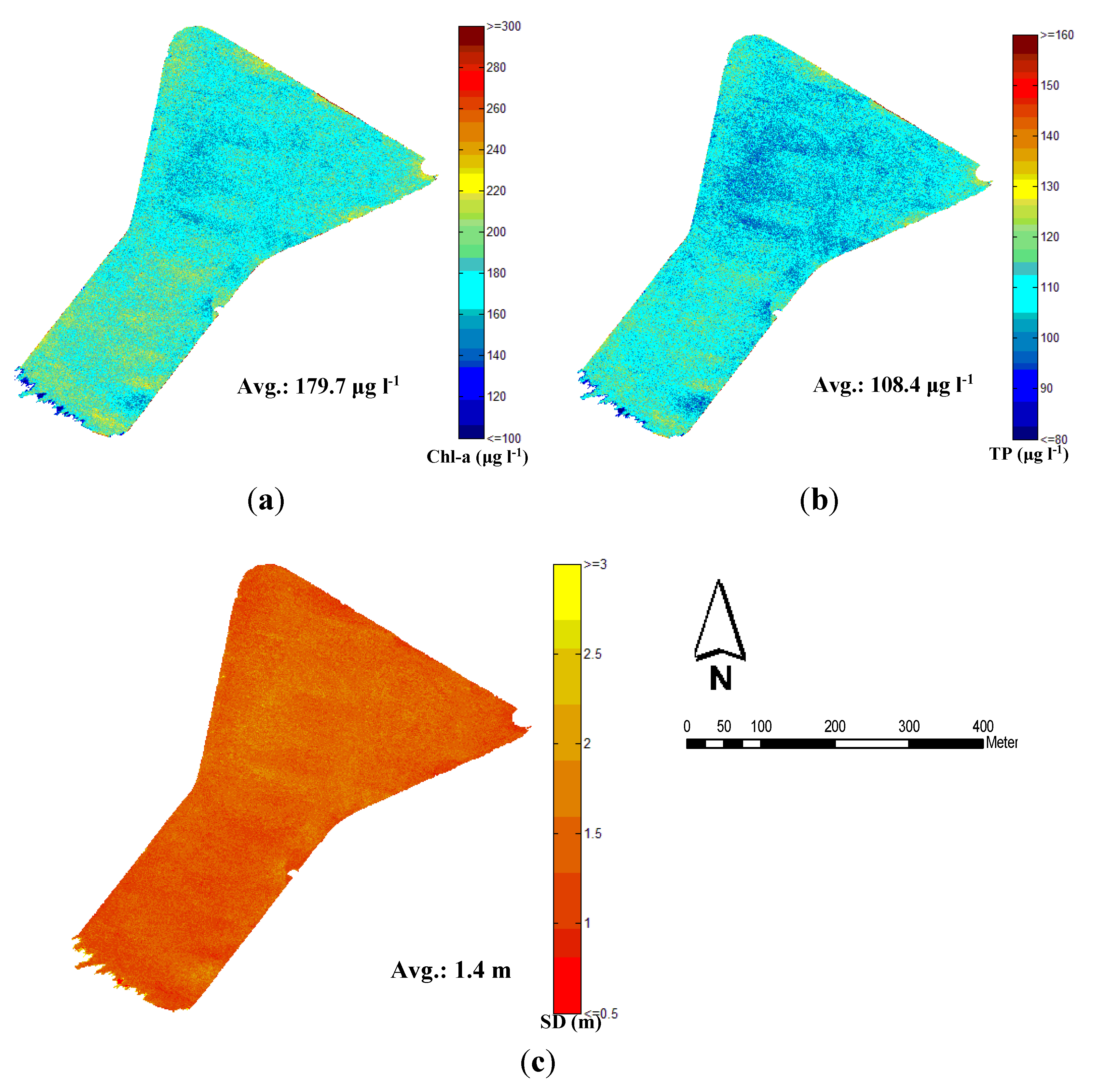
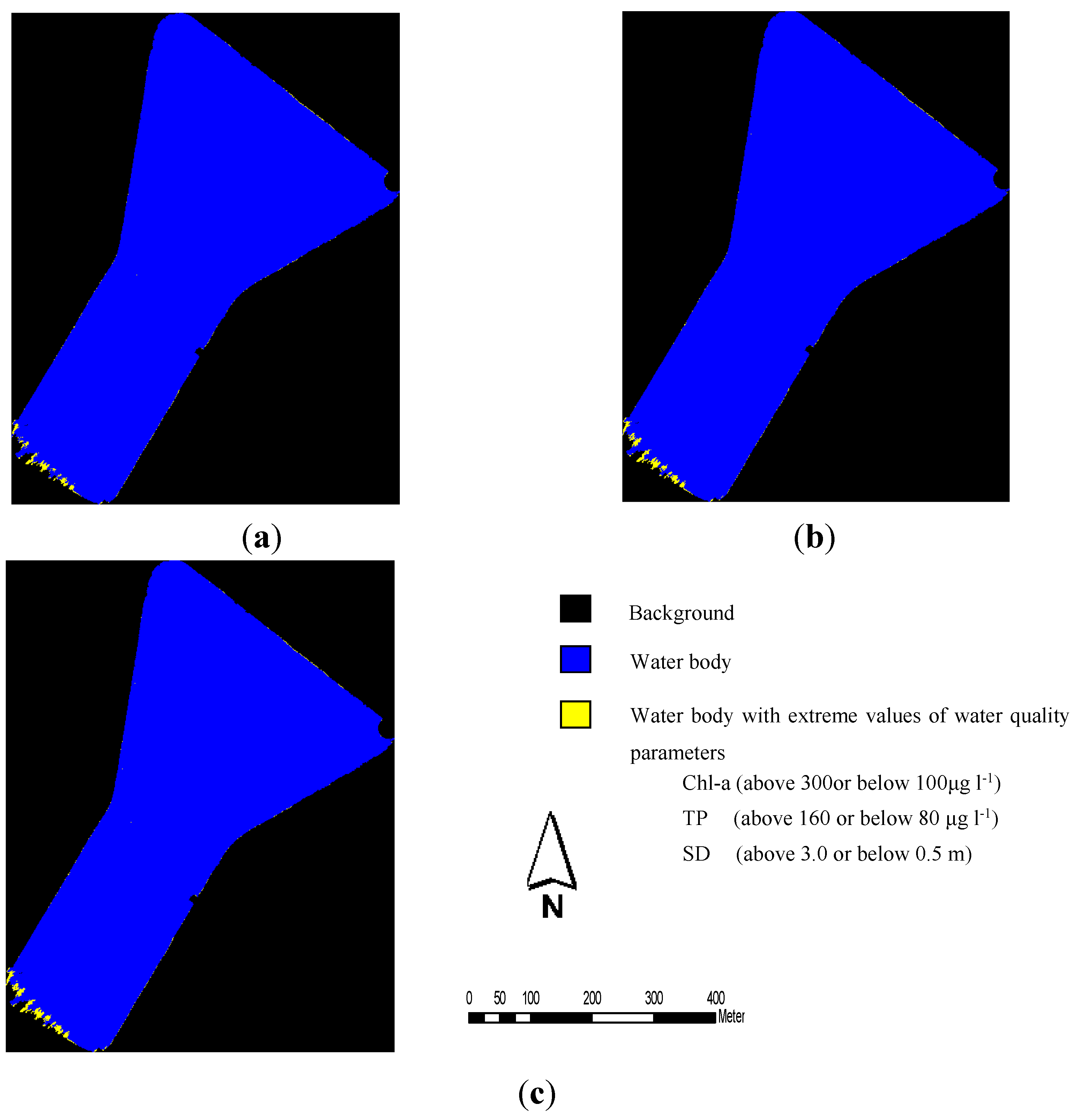
4.3. Trophic State of Tain-Pu Reservoir


5. Discussion
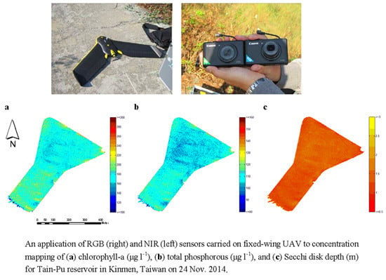
- Figure 6 shows that the higher concentrations of Chl-a or TP are distributed over the southwest side of Tain-Pu reservoir. Compared to the historical data of Chl-a and TP in the fall (see Table 1), with their examination data at sampling point 2 (see Table 3), i.e., the traditional sampling point, the concentrations of Chl-a and TP were significantly higher in the past years. We conjecture that the problem results from the current stream regulation project on the southwest side of Tain-Pu reservoir blocking the upstream water from flowing into the reservoir. Once the stream regulation project is finished, reinforcing the circulation of the water body is extremely important.
- Due to the hypereutrophic state of Tain-Pu reservoir, the current water body should be totally drained from the reservoir before receiving potable water from China. Simultaneously, the pollutant sources should be entirely surveyed and controlled to ensure that the reservoir has the capacity for self-oxidation.
6. Conclusions
Acknowledgments
Author Contributions
Conflicts of Interest
References
- Lillesand, T.M.; Johnson, W.L.; Deuell, R.L.; Lindstrom, O.M.; Meisner, D.E. Use of Landsat data to predict the trophic state of Minnesota Lakes. Photogramm. Eng. Remote Sens. 1983, 49, 219–229. [Google Scholar]
- Giardino, C.; Pepe, M.; Brivio, P.A.; Ghezzi, P.; Zilioli, E. Detecting chlorophyll, Secchi disk depth and surface temperature in a sub-alpine lake using Landsat imagery. Sci. Total Environ. 2001, 268, 19–29. [Google Scholar] [CrossRef]
- Vos, R.J.; Hakvoort, J.H.M.; Jordans, R.W.; Ibelings, B.W. Multiplatform optical monitoring of eutrophication in temporally and spatially variable lakes. Sci. Total Environ. 2003, 312, 221–243. [Google Scholar] [CrossRef]
- Erkkilä, A.; Kalliola, R. Patterns and dynamics of coastal waters in multi-temporal satellite images: Support to water quality monitoring in the Archipelago Sea, Finland. Estuar. Coast. Shelf Sci. 2004, 60, 165–177. [Google Scholar] [CrossRef]
- Sass, G.Z.; Creed, I.F.; Bayley, S.E.; Devito, K.J. Understanding variation in trophic status of lakes on the Boreal Plain: A 20year retrospective using Landsat TM imagery. Remote Sens. Environ. 2007, 109, 127–141. [Google Scholar] [CrossRef]
- Wang, Y.; Xia, H.; Fu, J.; Sheng, G. Water quality change in reservoirs of Shenzhen, China: Detection using LANDSAT/TM data. Sci. Total Environ. 2004, 328, 195–206. [Google Scholar] [CrossRef] [PubMed]
- Chen, L.; Tan, C.H.; Kao, S.J.; Wang, T.S. Improvement of remote monitoring on water quality in a subtropical reservoir by incorporating grammatical evolution with parallel genetic algorithms into satellite imagery. Water Res. 2008, 42, 296–306. [Google Scholar] [CrossRef] [PubMed]
- Wang, Z.; Hong, J.; Du, G. Use of satellite imagery to assess the trophic state of Miyun Reservoir, Beijing, China. Environ. Pollut. 2008, 155, 13–19. [Google Scholar]
- Schroeter, L.; Gläβer, C. Analyses and monitoring of lignite mining lakes in Eastern Germany with spectral signatures of Landsat TM satellite data. Int. J. Coal Geol. 2011, 86, 27–39. [Google Scholar] [CrossRef]
- Bonansea, M.; Rodriguez, M.C.; Pinotti, L.; Ferrero, S. Using multi-temporal Landsat imagery and linear mixed models for assessing water quality parameters in Río Tercero reservoir (Argentina). Remote Sens. Environ. 2015, 158, 28–41. [Google Scholar] [CrossRef]
- Palmer, S.C.J.; Kutser, T.; Hunter, P.D. Remote sensing of inland waters: Challenges, progress and future directions. Remote Sens. Environ. 2015, 157, 1–8. [Google Scholar] [CrossRef]
- Yang, M.D.; Sykes, R.M.; Merry, C.J. Estimation of algal biological parameters using water quality modeling and SPOT satellite data. Ecol. Model. 2000, 125, 1–13. [Google Scholar] [CrossRef]
- Dekker, A.G.; Vos, R.J.; Peters, S.W.M. Analytical algorithms for lake water TSM estimation for retrospective analyses of TM and SPOT sensor data. Int. J. Remote Sens. 2002, 23, 15–35. [Google Scholar] [CrossRef]
- Tarrant, P.E.; Amacher, J.A.; Neuer, S. Assessing the potential of Medium-Resolution Imaging Spectrometer (MERIS) and Moderate-Resolution Imaging Spectroradiometer (MODIS) data for monitoring total suspended matter in small and intermediate sized lakes and reservoirs. Water Resour. Res. 2010, 46. [Google Scholar] [CrossRef]
- Olmanson, L.G.; Brezonik, P.L.; Bauer, M.E. Evaluation of medium to low resolution satellite imagery for regional lake water quality assessments. Water Resour. Res. 2011, 47. [Google Scholar] [CrossRef]
- Huang, C.; Wang, X.; Yang, H.; Li, Y.; Wang, Y.; Chen, X.; Xu, L. Satellite data regarding the eutrophication response to human activities in the plateau lake Dianchi in China from 1974 to 2009. Sci. Total Environ. 2014, 485–486, 1–11. [Google Scholar] [CrossRef] [PubMed]
- Michaelsen, E.; Meidow, J. Stochastic reasoning for structural pattern recognition: An example from image-based UAV navigation. Pattern Recognit. 2014, 47, 2732–2744. [Google Scholar] [CrossRef]
- Niethammer, U.; James, M.R.; Rothmund, S.; Travelletti, J.; Joswig, M. UAV-based remote sensing of the Super-Sauze landslide: Evaluation and results. Eng. Geol. 2012, 128, 2–11. [Google Scholar] [CrossRef]
- Zarco-Tejada, P.J.; González-Dugo, V.; Berni, J.A.J. Fluorescence, temperature and narrow-band indices acquired from a UAV platform for water stress detection using a micro-hyperspectral imager and a thermal camera. Remote Sens. Environ. 2012, 117, 322–337. [Google Scholar] [CrossRef]
- Zarco-Tejada, P.J.; Guillen-Climent, M.L.; Hernandez-Clemente, R.; Catalina, A.; Gonzalez, M.R.; Martin, P. Estimating leaf carotenoid content in vineyards using high resolution hyperspectral imagery acquired from an unmanned aerial vehicle (UAV). Agric. Forest Meteorol. 2013, 171–172, 281–294. [Google Scholar] [CrossRef]
- Colomina, I.; Molina, P. Unmanned aerial systems for photogrammetry and remote sensing: A review. ISPRS J. Photogramm. Remote Sens. 2014, 92, 79–97. [Google Scholar] [CrossRef]
- Immerzeel, W.W.; Kraaijenbrink, P.D.A.; Shea, J.M.; Shrestha, A.B.; Pellicciotti, F.; Bierkens, M.F.P.; de Jong, S.M. High-resolution monitoring of Himalayan glacier dynamics using unmanned aerial vehicles. Remote Sens. Environ. 2014, 150, 93–103. [Google Scholar] [CrossRef]
- Peter, K.D.; d’Oleire-Oltmanns, S.; Ries, J.B.; Marzolff, I.; Hssaine, A.A. Soil erosion in gully catchments affected by land-levelling measures in the Souss Basin, Morocco, analysed by rainfall simulation and UAV remote sensing data. Catena 2014, 113, 24–40. [Google Scholar] [CrossRef]
- Torres-Sanchez, J.; Pena, J.M.; de Castro, A.I.; Lopez-Granados, F. Multi-temporal mapping of the vegetation fraction in early-season wheat fields using images from UAV. Comput. Electron. Agric. 2014, 103, 104–113. [Google Scholar] [CrossRef]
- Bendig, J.; Yu, K.; Aasen, H.; Bolten, A.; Bennertz, S.; Broscheit, J.; Gnyp, M.L.; Bareth, G. Combining UAV-based plant height from crop surface models, visible, and near infrared vegetation indices for biomass monitoring in barley. Int. J. Appl. Earth Obs. Geoinf. 2015, 39, 79–87. [Google Scholar] [CrossRef]
- Flynn, K.F.; Chapra, S.C. Remote sensing of submerged aquatic vegetation in a shallow non-turbid river using an unmanned aerial vehicle. Remote Sens. 2014, 6, 12815–12836. [Google Scholar] [CrossRef]
- Pajares, G. Overview and current status of remote sensing applications based on unmanned aerial vehicles (UAVs). Photogramm. Eng. Remote Sens. 2015, 81, 281–330. [Google Scholar]
- Pavluk, T.; bij de Vaate, A. Trophic index and efficiency. In Encyclopedia of Ecology; Jorgensen, S.E., Fath, B., Eds.; Elsevier: Amsterdam, The Netherlands, 2008; pp. 3602–3608. [Google Scholar]
- Zhao, D.; Cai, Y.; Jiang, H.; Xu, D.; Zhang, W.; An, S. Estimation of water clarity in Taihu Lake and surrounding rivers using Landsat imagery. Adv. Water Resour. 2011, 34, 165–173. [Google Scholar] [CrossRef]
- Environmental Analysis Laboratory, EPA, Taiwan. Available online: http://www.niea.gov.tw/analysis/method/ListMethod.asp?methodtype=LIVE (accessed on 28 June 2015).
- Carlson, R.E. A trophic state index for lakes. Limnol. Oceanogr. 1997, 22, 361–369. [Google Scholar] [CrossRef]
- Wolf, P.R.; Dewitt, B.A. Elements of Photogrammetry with Applications in GIS, 3rd ed.; McGraw-Hill: Taipei, Taiwan, 2000. [Google Scholar]
- Lillesand, T.M.; Kiefer, R.W.; Chipman, J.W. Remote Sensing and Image Interpretation, 6th ed.; Wiley: NJ, USA, 2008. [Google Scholar]
- Doña, C.; Chang, N.B.; Caselles, V.; Sánchez, J.M.; Camacho, A.; Delegido, J.; Vannah, B.W. Integrated satellite data fusion and mining for monitoring lake water quality status of the Albufera de Valencia in Spain. J. Environ. Manag. 2015, 151, 416–426. [Google Scholar] [CrossRef] [PubMed]
- Zaman, B.; Jensen, A.; Clemens, S.R.; McKee, M. Retrieval of spectral reflectance of high resolution multispectral imagery acquired with an autonomous unmanned aerial vehicle: AggieAirTM. Photogramm. Eng. Remote Sens. 2014, 80, 1139–1150. [Google Scholar]
- Chipman, J.W.; Olmanson, L.G.; Gitelson, A.A. Remote Sensing Methods for Lake Management: A Guide for Resource Managers and Decision-Makers; Developed by the North American Lake Management Society in Collaboration with Dartmouth College, University of Minnesota, and University of Nebraska, for the United States Environmental Protection Agency: Madison, WI, USA, 2009. [Google Scholar]
- Kloiber, S.M.; Brezonik, P.L.; Olmanson, L.G.; Bauer, M.E. Application of Landsat imagery to regional-scale assessments of lake clarity. Water Res. 2002, 36, 4330–4340. [Google Scholar] [CrossRef]
- Chipman, J.W.; Lillesand, T.M.; Schmaltz, J.E.; Leale, J.E.; Nordheim, M.J. Mapping lake clarity with Landsat images in Wisconsin, U.S.A. Can. J. Remote Sens. 2004, 30, 1–7. [Google Scholar] [CrossRef]
- Olmanson, L.G.; Bauer, M.E.; Brezonik, P.L. A 20-year Landsat water clarity census of Minnesota’s 10,000 lakes. Remote Sens. Environ. 2008, 112, 4086–4097. [Google Scholar] [CrossRef]
- McCullough, I.M.; Loftin, C.S.; Sader, S.A. High-frequency remote monitoring of large lakes with MODIS 500 m imagery. Remote Sens. Environ. 2012, 124, 234–241. [Google Scholar] [CrossRef]
- Tebbs, E.J.; Remedios, J.J.; Harper, D.M. Remote sensing of chlorophyll-a as a measure of cyanobacterial biomass in Lake Bogoria, a hypertrophic, saline–alkaline, Flamingo Lake, using Landsat ETM+. Remote Sens. Environ. 2013, 135, 92–106. [Google Scholar] [CrossRef]
- Matthews, M.W. A current review of empirical procedures of remote sensing in inland and near-coastal transitional waters. Int. J. Remote Sens. 2011, 32, 6855–6899. [Google Scholar] [CrossRef]
- Sriwongsitanon, N.; Surakit, K.; Thianpopirug, S. Influence of atmospheric correction and number of sampling points on the accuracy of water clarity assessment using remote sensing application. J. Hydrol. 2011, 401, 203–220. [Google Scholar] [CrossRef]
© 2015 by the authors; licensee MDPI, Basel, Switzerland. This article is an open access article distributed under the terms and conditions of the Creative Commons Attribution license (http://creativecommons.org/licenses/by/4.0/).
Share and Cite
Su, T.-C.; Chou, H.-T. Application of Multispectral Sensors Carried on Unmanned Aerial Vehicle (UAV) to Trophic State Mapping of Small Reservoirs: A Case Study of Tain-Pu Reservoir in Kinmen, Taiwan. Remote Sens. 2015, 7, 10078-10097. https://doi.org/10.3390/rs70810078
Su T-C, Chou H-T. Application of Multispectral Sensors Carried on Unmanned Aerial Vehicle (UAV) to Trophic State Mapping of Small Reservoirs: A Case Study of Tain-Pu Reservoir in Kinmen, Taiwan. Remote Sensing. 2015; 7(8):10078-10097. https://doi.org/10.3390/rs70810078
Chicago/Turabian StyleSu, Tung-Ching, and Hung-Ta Chou. 2015. "Application of Multispectral Sensors Carried on Unmanned Aerial Vehicle (UAV) to Trophic State Mapping of Small Reservoirs: A Case Study of Tain-Pu Reservoir in Kinmen, Taiwan" Remote Sensing 7, no. 8: 10078-10097. https://doi.org/10.3390/rs70810078