
Automatic Geometry Generation from Point Clouds for BIM


Civil, Environmental & Geomatic Engineering, University College London, Gower Street, London WC1E 6BT, UK
*
Author to whom correspondence should be addressed.
Remote Sens. 2015, 7(9), 11753-11775; https://doi.org/10.3390/rs70911753
Submission received: 21 June 2015
/
Revised: 3 September 2015
/
Accepted: 8 September 2015
/
Published: 14 September 2015
(This article belongs to the Special Issue Remote Sensed Data and Processing Methodologies for 3D Virtual Reconstruction and Visualization of Complex Architectures)
Abstract
:The need for better 3D documentation of the built environment has come to the fore in recent years, led primarily by city modelling at the large scale and Building Information Modelling (BIM) at the smaller scale. Automation is seen as desirable as it removes the time-consuming and therefore costly amount of human intervention in the process of model generation. BIM is the focus of this paper as not only is there a commercial need, as will be shown by the number of commercial solutions, but also wide research interest due to the aspiration of automated 3D models from both Geomatics and Computer Science communities. The aim is to go beyond the current labour-intensive tracing of the point cloud to an automated process that produces geometry that is both open and more verifiable. This work investigates what can be achieved today with automation through both literature review and by proposing a novel point cloud processing process. We present an automated workflow for the generation of BIM data from 3D point clouds. We also present quality indicators for reconstructed geometry elements and a framework in which to assess the quality of the reconstructed geometry against a reference.

1. Introduction
The main techniques for capturing 3D data about the built environment from terrestrial platforms are through laser scanning or total station measurements. The latter being the predominant method for building surveys where a predetermined set of point measurements are taken of features from which 2D CAD plans are produced. Terrestrial laser scanning has been the technology of choice for the 3D capture of complex structures that are not easily measured with the sparse but targeted point collection from a total station since the technology was commercialised around 2000. This includes architectural façades with very detailed elements and refineries or plant rooms where the nature of the environment to be measured makes traditional workflows inefficient. This is particularly exemplified in the increased use of freeform architecture by prominent architects such as Frank Gehry and Zaha Hadid [1] where laser scanning presents the most viable option for timely data capture of complex forms.
Building Information Modelling (BIM) is the digital data flow surrounding the lifecycle of an asset or element of the built environment, instigated to provide better information management to aid with decision making. As a process, BIM has been gaining global acceptance across the Architecture, Engineering, Construction, and Operations (AECO) community for improving information sharing about built assets. A key component of this is a data-rich object-based 3D parametric model that holds both geometric and semantic information. By creating a single accessible repository of data, then other tools can be utilised to extract useful information about the asset for various purposes.
Although BIM has been extensively studied from the new build process, it is in retrofit where it is likely to provide the greatest impact. In the UK alone, at least half of all construction by cost is on existing assets [2]. With the need to achieve international environmental targets and construction being one of the largest contributors of CO2 emissions in the UK, sustainable retrofit is only going to become more relevant. This is supported by the estimate of the UK Green Building Council that of total building stock in the UK, the majority will still exist in 2050 [3]. Therefore, many existing buildings will need to be made more environmentally efficient if the Government is to reach its sustainability targets.
With the introduction of BIM and the data-rich 3D parametric object model at its heart, laser scanning has come to the fore as the primary means of data capture. This has been aided by both the US and UK Governments advising that laser scanning should be the capture method of choice for geometry [4,5]. However, little thought has been given about how to integrate this in to the BIM process due to the change in the nature of the information requirements of a BIM model and uncertainty over level of detail or information that should be provided by a Geomatic Land Surveyor. It has been proposed that a point cloud represents an important lowest level of detail base (stylised as LoD 0) from which more information rich abstractions can be generated representing higher levels of detail [6].
Traditional surveying with scanning currently does not result in a product that is optimal for the process of BIM due to the historical use of non-parametric CAD software to create survey plans. Therefore, a process shift is required in workflows and modelling procedures of the stakeholders who do this work to align themselves with this. The shorthand name given to the survey process of capture to model is Scan to BIM. Technically Scan to BIM as a phrase is wrongly formed as the end result is not BIM as usually understood, i.e. the process, but a 3D parametric object model that aids the process at its current level of development.
Even though, from a BIM perspective, creating parametric 3D building models from scan data appears new, it actually extends back to the early days of commercialised terrestrial laser scanning systems creating parameterised surface representations from segmented point clouds [7] and goes back further than this in the aerial domain for external parametric reconstruction [8,9]. A system of note from the close-range photogrammetry domain is Hazmap; originally developed to facilitate the capture and parametric modelling of complex nuclear plants in the 1990s [10]. Hazmap consisted of a panoramic imaging system using calibrated cameras attached to a robotic total station. This would capture 60 images per setup and use a full bundle adjustment together with total station measurements for scale to localise the sensor setup positions. After capture, the system made use of a plant design and management system (PDMS) interface that allowed the user to take measurements in the panoramic imagery and export them via a macro to the PDMS where the plant geometry could be modelled using a library of parametric elements.
One of the earliest pieces of research with a workflow that would be recognised today as scan to BIM is in [11]. Their key conclusion was to consider what tolerance is acceptable both in surveying and modelling as assuming orthogonality is rarely true in retrofit but may be desirable to simplify the modelling process.
1.1. Standards for Modelling
The survey accuracy requirement set by the Royal Institution of Chartered Surveyors (RICS) was for 4cm accuracy for building detail design at a drawing resolution of 20 cm [12]. However, in a 3D modelling context, drawing resolution now seems less relevant and so in 2014 an updated guidance note was published splitting accuracy into plan and height with measured building surveys banded between ±4–25 mm depending on job specification [13]. We choose the RICS over other guidelines such as those for the survey of historic buildings, as our work focuses more on the modelling of contemporary buildings where RICS is more relevant.
Before this updated guidance, a UK survey specification for a BIM context did not exist. Therefore, survey companies took it upon themselves to create in-house guides. The most comprehensive of these is by Plowman Craven who freely released their specification, focused around the parametric building modeller Revit, and documenting what they as a company will deliver in terms of the geometric model [14].
One of the immediate impressions of this document is the number of caveats that it contains with respect to the geometry and how the model deviates from reality. This is partially due to the reliance on Revit and the orthogonal design constraints that this encourages, meaning that representing unusual deviations that exist in as-built documentation have to be accounted for in this way; unless very time consuming (and therefore expensive) bespoke modelling is performed. This experience is borne out by literature where the tedium of modelling unique components [11] and the unsuitability of current BIM software to represent irregular geometry such as walls out of plumb [15] are recognised. However Plowman Craven, as outlined in their specification above, do make use of the availability of rich semantic detail to add quality information about deviations from the point cloud to the modelled elements. In the medium to long term, the establishment of the point cloud as a fundamental data model is likely to happen as models and the data they are derived from start to exist more extensively together in a BIM environment.
Larsen et al. [15] endorses this view and considers that the increased integration of point clouds into BIM software makes post processing redundant. However, they then contradict this by envisaging that a surveyor provides a "registered, cleaned and geo-referenced point cloud". By post processing, Larsen et al. appear to be referring to the modelling process and see the filtering and interpretation of data to be obsolete with the point cloud a "mould" that other professions in the lifecycle can make use of as necessary.
1.2. Current State of the Art
Automated modelling is seen as desirable commercially to reduce time and therefore cost and make scanning a more viable proposition for a range of tasks in the lifecycle, such as daily construction change detection [16,17].
Generally, digital modelling is carried out to provide a representation or simulation of an entity that does not exist in reality. However for existing buildings, the goal is to model entities as they exist in reality. Currently the process is very much a manual one and recognised by many as being time-consuming, tedious, subjective and requiring skill [11,18]. The general manual process as in creating 2D CAD plans, from point clouds requires the operator to use the cloud as a guide in a BIM tool to effectively trace around the geometry, requiring a high knowledge input to interpret the scene as well as add the rich semantic information that really makes BIM a valuable process.
The orthogonal constraints present in many BIM design tools limit the modelling that can be achieved without intense operator input. Depending on the type and use of the model this is not necessarily a disadvantage. In many cases a geometric representation is not required to have very tight tolerances [7]. This further emphasises the need to define fitness for purpose and we have given some examples of UK standards and specifications above.
1.2.1. Research
Both Computer Science and Geomatics are investigating the automated reconstruction of geometry from point clouds, especially as interior modelling has risen in prominence with the shift to BIM requiring rich parametric models. Geomatics has a track record in this with reconstruction from facades, pipework and from aerial LIDAR data as in [19,20]. An early review of methods is given by [21].
The ideas and approaches taken to aiding the problem of geometry reconstruction have mainly come from computer science. This community uses parametric modelling as a paradigm mainly implemented for invented or stylised representations of the externals of buildings using techniques such as procedural modelling and grammars, i.e. algorithms to generate the model [22]. This rule-based approach to automating the modelling process can fit well to the parametric models that are intrinsically rule driven; [23] presents this approach. Rules can also be represented by shape grammars as shown by [24].
The focus of computer science on BIM has mainly been on algorithms to speed the modelling of geometry from point clouds, as well as applying other vision techniques from robotics for scene understanding. This is all related to automating the understanding of the environment, which is an important prerequisite for providing robots with autonomy [25].
In terms of the reconstruction of building elements, the focus has been on computational geometry algorithms to extract the 3D representation of building elements through segmentation, including surface normal approaches [26], plane sweeping [27] and region growing [28]. Segmentation of range measurement data is a long established method (initially from computer vision for image processing) for classifying data with the same characteristics together. An example of this is Hoover et al. [29],which brought together the different approaches to this topic that were being pursued at the time and presented a method for evaluating these segmentation algorithms.
Existing work that has shown promising results towards automating the reconstruction process of geometry include [30,31], however these do not result in a parametric object-based model as used in BIM but in a 3D CAD model that needs to be remodelled manually, a point made by Volk et. al. [32] who provide an extensive review of the area.
However Nagel et al. [33] points out that the full automatic reconstruction of building models has been a topic of research for many groups over the last 25 years with little success to date. They suggest the problem is with the high reconstruction demands due to four issues: definition of a target structure that covers all variations of building, the complexity of input data, ambiguities and errors in the data, and the reduction of the search space during interpretation.
1.2.2. Commercial
Given the above statement about achieving full automation, there are a few commercial pieces of software that have emerged in recent years and could be described as semi-automated. To the best of the authors’ knowledge all these tools rely on Autodesk Revit for the geometry generation. Below the prominent packages are summarised.
The first is by ClearEdge3D who provides solutions for plant and MEP object detection alongside a building-focused package called Edgewise Building. This classifies the point cloud into surfaces that share coplanar points, with the operator picking floor and ceiling planes to constrain the search for walls [34]. Once found, this geometry can be bought into Revit via a plugin to construct the parametric object-based geometry. In its wall detection, Edgewise uses the scan locations to aid geometric reasoning; a constraint it forces by only allowing file-per-scan point clouds for processing.
The other main solution is Scan to BIM from IMAGINiT Technologies, which is perhaps the most successful solution in terms of deliverable [35]. This is a plugin to Revit and therefore relies on much of the functionality of Revit to handle most tasks (including loading the point cloud and geometry library) and essentially just adds some detection and fitting algorithms along with a few other tools for scan handling. The main function is wall fitting whereby the user picks three points to define the wall plane from which a region growing algorithm detects the extents. The user then sets a tolerance and selects which parametric wall type element in the Revit model should be used. There is also the option of fitting a mass wall, which is a useful way of modelling a wall face that is not perfectly plumb and orthogonal. The downside to this plugin is that it only handles definition by one surface meaning that one side of a wall has to be relied upon to model the entire volume, unless one fitted a mass wall from each surface and did a Boolean function to merge the two solids appropriately.
Kubit, now owned by Faro, and Pointcab both provide tools that aid the manual process of tracing the points in Autodesk software but do not, as of this time, automate the geometry production [36,37]. Autodesk itself did trial its own Revit module for automated building element creation from scan data, which it shared with users through its Autodesk Labs preview portal. However, this module is no longer available and it remains to be seen if this will ever be integrated into future production editions of Revit.
2. Proposed Method
In the following, we describe our methods to automate the identification of geometric objects from point clouds and vice versa. We concentrate on the major room bounding entities, i.e., walls. Other more detailed geometric objects such as windows and doors are not currently considered.
2.1. Overview
Two methods are presented in this paper, one to automatically reconstruct basic Industry Foundation Classes (IFC) geometry from point clouds and another to classify a point cloud given an existing IFC model. The former consists of three main components:
- (1)
- Reading the data into memory for processing
- (2)
- Segmentation of the dominant horizontal and vertical planes
- (3)
- Construct the IFC geometry
While the latter consists of two:
- (1)
- Reading the IFC objects bounding boxes from the file
- (2)
- Use the bounding boxes to segment the point cloud by object
By using E57 for the scans and IFC for the intelligent BIM geometry, this work is kept format agnostic, as these are widely accepted open interchange formats, unlike the commercial solutions which overly rely on Autodesk Revit for their geometry creation. IFC was developed out of the open CAD format STEP, and uses the EXPRESS schemata to form an interoperable format for information about buildings. This format is actively developed as a recognised open international standard for BIM data: ISO 16739 [38]. Within IFC, building components are stored as instances of objects that contain data about themselves. This data includes geometric descriptions (position relative to building, geometry of object) and semantic ones (description, type, relation with other objects) [39].
This work makes use of two open source libraries as a base from which the routine presented has been built up. The first is the Point Cloud Library (PCL) version 1.7.0, which provides a number of data handling and processing algorithms for point cloud data [40]. The second is the eXtensible Building Information Modelling (xBIM) toolkit version 2.4.1.28, which provides the ability to read, write and view IFC files compliant with the IFC2x3 TC1 standard [41].
2.2. Point Cloud to IFC
2.2.1. Reading In
Loading the point cloud data into memory is the first step in the process. To keep with the non-proprietary, interoperable nature of BIM the E57 format was decided as the input format of choice to support. The LIBE57 library version 1.1.312 provided the necessary reader to interpret the E57 file format [42] and some code was written to transfer the E57 data into the PCL point cloud data structure. In this case, only the geometry was needed so only the coordinates were taken into the structure.
2.2.2. Plane Model Segmentation
With the data loaded in, the processing can begin. Firstly the major horizontal planes are detected as these likely represent the floor and ceiling components and then the vertical planes which likely represent walls (Figure 1b,c). The plane detection for both cases is done with the PCL implementation of RANSAC (RANdom SAmple Consensus) [43] due to the speed and established nature. The algorithm is constrained to accept only planes whose normal coefficient is within a three degree deviation from parallel to the Z-axis (up) for horizontal planes and perpendicular to Z for vertical planes. Also a distance threshold was set for the maximum distance of the points to the plane to accept as part of the model. Choosing this value is related to the noise level of the data from the instrument that was used for capture. As a result, the stopping criteria for each RANSAC run is when a plane is found with 99% confidence consisting of the most inliers within tolerance. This is an opportunistic or “greedy” approach, based on the assumption that the largest amount of points that most probably fit a plane will be the building element. This approach can lead to errors especially where the plane is more ambiguous, but is fast and simple to implement. Recent developments could improve this such as Monszpart et al. [44], which provides a formulation that allows less dominant planes to not become lost in certain scenes.
Figure 1.
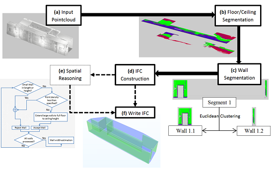
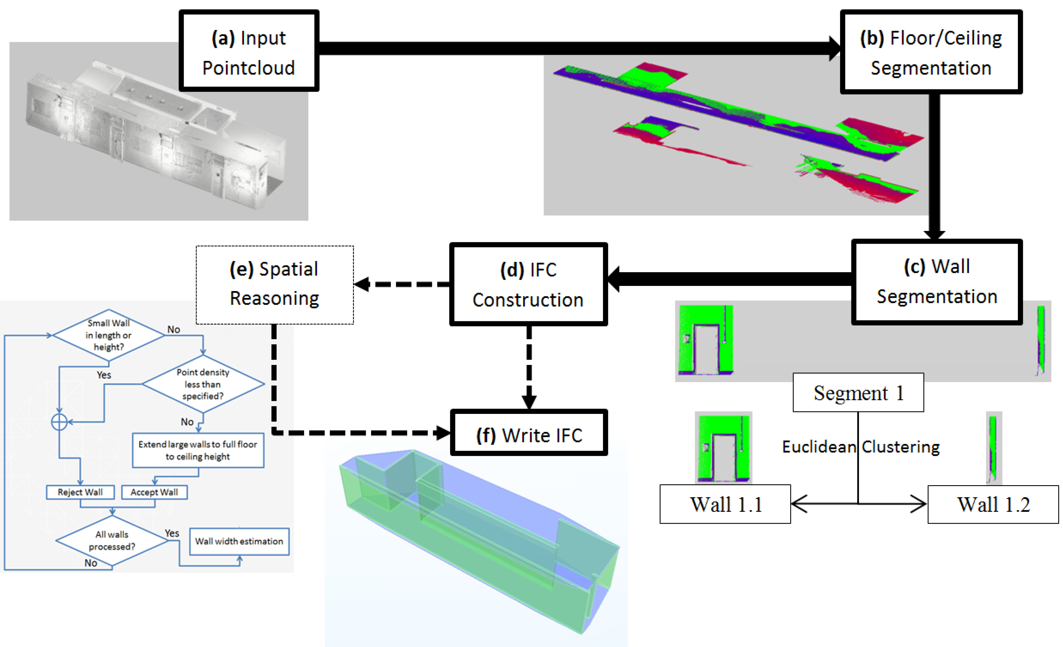
Flowchart of Point Cloud to IFC algorithm steps. (a) Load Point Cloud; (b) Segment the Floor and Ceiling Planes; (c) Segment the Walls and split them with Euclidean Clustering; (d) Build IFC Geometry from Point Cloud segments; (e) (Optional) Spatial reasoning to clean up erroneous geometry; (f) Write the IFC data to an IFC file.
Figure 1.
Flowchart of Point Cloud to IFC algorithm steps. (a) Load Point Cloud; (b) Segment the Floor and Ceiling Planes; (c) Segment the Walls and split them with Euclidean Clustering; (d) Build IFC Geometry from Point Cloud segments; (e) (Optional) Spatial reasoning to clean up erroneous geometry; (f) Write the IFC data to an IFC file.

The downside to extracting points that conform to a planar model using RANSAC alone is that the algorithm extracts all of the points within tolerance across the whole plane model, irrelevant of whether they form part of a contiguous plane. Therefore a Euclidean Clustering step [45] was introduced after the RANSAC to separate the contiguous elements out, as it could not be assumed that two building elements that shared planar coefficients but were separate in the point cloud represented the same element (Figure 1c). Euclidean Clustering separates the point data into sets based on their distance to each other up to a defined tolerance. Along with this, a constraint or condition was applied to preserve planarity, preventing points that lay on the plane but formed part of a differently oriented surface from being included. The constraint manifested as the dot product between the normal ranges of each point added to the clusters had to be close to parallel. Accepted clusters to extract are chosen based on the amount of points assigned to the cluster as a percentage of the total data set.
With the relevant points that represent dominant planes extracted, the requisite dimensions needed for IFC geometry construction could be measured. This meant extracting a boundary for the slabs and a length and height extent for the walls; the reasons for this are provided in the next section.
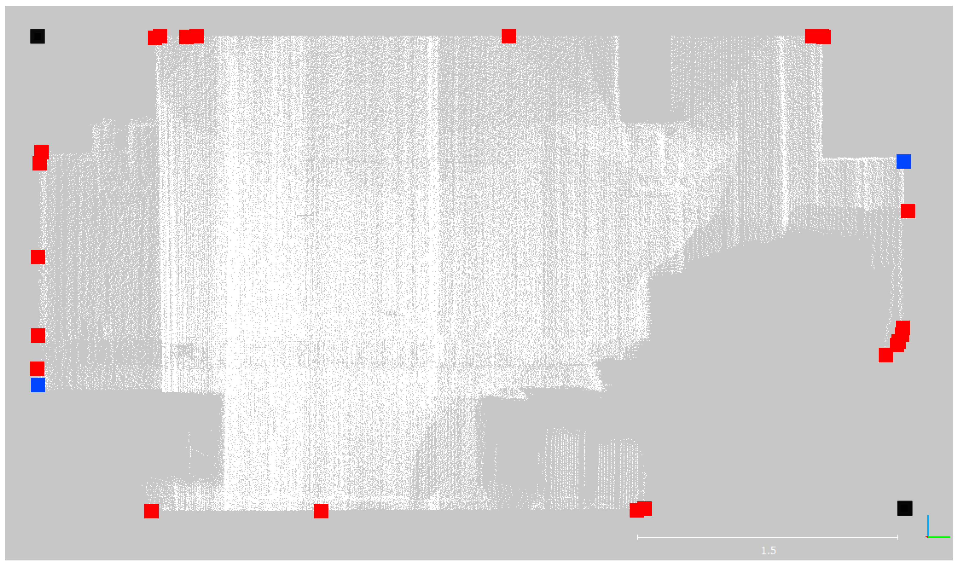
Once all clusters are extracted, further information for each is collected. For each slab’s cluster, the points are projected onto the RANSAC-derived plane. The convex hull in the planar projection is calculated to give the coordinates of the boundary. The two corner points that describe the maximum extent of the cluster are computed to describe the wall (Figure 2). This finds the extent well along the X/Y direction (blue points of Figure 2), but the height of the wall cannot be guaranteed to be found by this method. This situation is illustrated in Figure 2, because parts of the wall can extend further than the places of maximum and minimum height. To counter this, the minimum and maximum Z coordinates (height) were sought by sorting all the coordinates and returning both the lowest and the highest values. By using these Z values, an overall wall extent can be defined (black points of Figure 2).
Figure 2.
Example plot of minimum and maximum (black) and maximum segment (blue) coordinates on the points of a convex hull (red) calculated for a wall cluster point cloud (white).
Figure 2.
Example plot of minimum and maximum (black) and maximum segment (blue) coordinates on the points of a convex hull (red) calculated for a wall cluster point cloud (white).

2.2.3. IFC Generation
Each IFC object can be represented a few different ways (swept solid, brep, etc.) To create the IFC, the geometry of the elements needs to be constructing using certain dimensions. In this work the IFC object chosen for wall representation is IfcWallStandardCase, which handles all walls that are described by a vertically extruded footprint. The slab representation chosen is IfcSlab, defined similarly to the walls by extruding a 2D perimeter of coordinates vertically down by a value [46].
We start by creating an initializing an empty model into which the IFC objects can be added. Each object is created from the information extracted previously by the segmentation code detailed in the last section. First the slabs are added by providing a boundary, extrusion depth or thickness and the level in Z at which he slab is extruded from. The walls are represented by their object dimensions (length, width, height) and a placement coordinate and rotation (bearing) of that footprint in the global coordinate system. As the usefulness of BIM is as much about the semantic information alongside the geometry, mean and standard deviation information on the RANSAC plane fits is added as a set of properties to the geometry of walls and slabs.
2.2.4. Spatial Reasoning
An optional step of geometric reasoning can be added to the IFC generation process to clean up the reconstructed geometry (Figure 1e). This implements some rules or assumptions about the reconstructed elements to change or remove them from the model. The following rules have been implemented and can be customized by user-defined thresholds.
- Reject small walls: Planes that are too small in length or occupy too little of the height between floor and ceiling levels are removed from the model. For the experiments described here we chose 100mm as the minimum length and 1/3 of the floor to ceiling distance as the minimum height.
- Extend large walls: Large planes which do not extend fully from floor to ceiling are automatically extended so their lowest height is at floor level and highest is at ceiling level. For the experiments we chose walls that are greater than 1m in length or occupy 2/3 of the height between floor and ceiling levels.
- Merge close planes with similar normal: Planes that have parallel normals and within an offset distance from each other are merged into one wall of overall thickness being the distance between the planes. If a plane pair is not found a default value of 100mm thickness is used. For the experiments we chose a distance threshold of 300mm. This currently relies on user input but a database of priors that would be expected in the building would streamline this.
Once successfully created with or without geometric reasoning applied the walls and slabs can be stored to the model and saved as an IFC file. Figure 3 shows an example of the resultant geometry that is obtained through both processes. This file can then be viewed in any IFC viewer or BIM design tools such as Autodesk Revit.
2.3. IFC to Point Cloud
The process described in the previous section of generating the geometry can, in effect, be reversed and the model used to extract elements out of the point cloud within a tolerance. In so doing, these segments of the point cloud can be classified and assessed for their quality of representation in the model based on the underlying point cloud data that occupies that geometric space. This process could easily be the start of a facilitation process towards 4D change detection as a project evolves on site against a scheduled design model for that time epoch.
Figure 3.
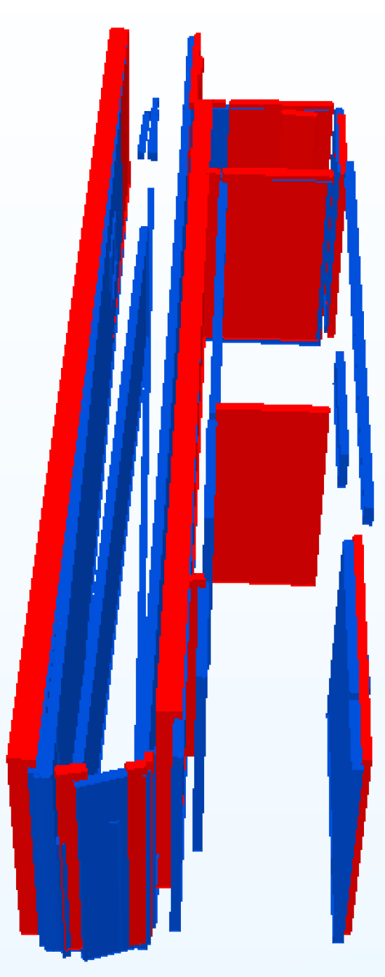
Example of corridor reconstruction without (blue) and with (red) spatial reasoning applied.
Figure 3.
Example of corridor reconstruction without (blue) and with (red) spatial reasoning applied.

2.3.1. Reading the IFC
We start by loading the IFC file into memory. Then, for each IFC object that is required, the coordinates of an object-oriented bounding box are extracted as the return geometry. A user specified tolerance can be added to take account of errors and generalisations made during modelling, thus enlarging the bounding boxes by that amount.
2.3.2. Classifying the Point Cloud
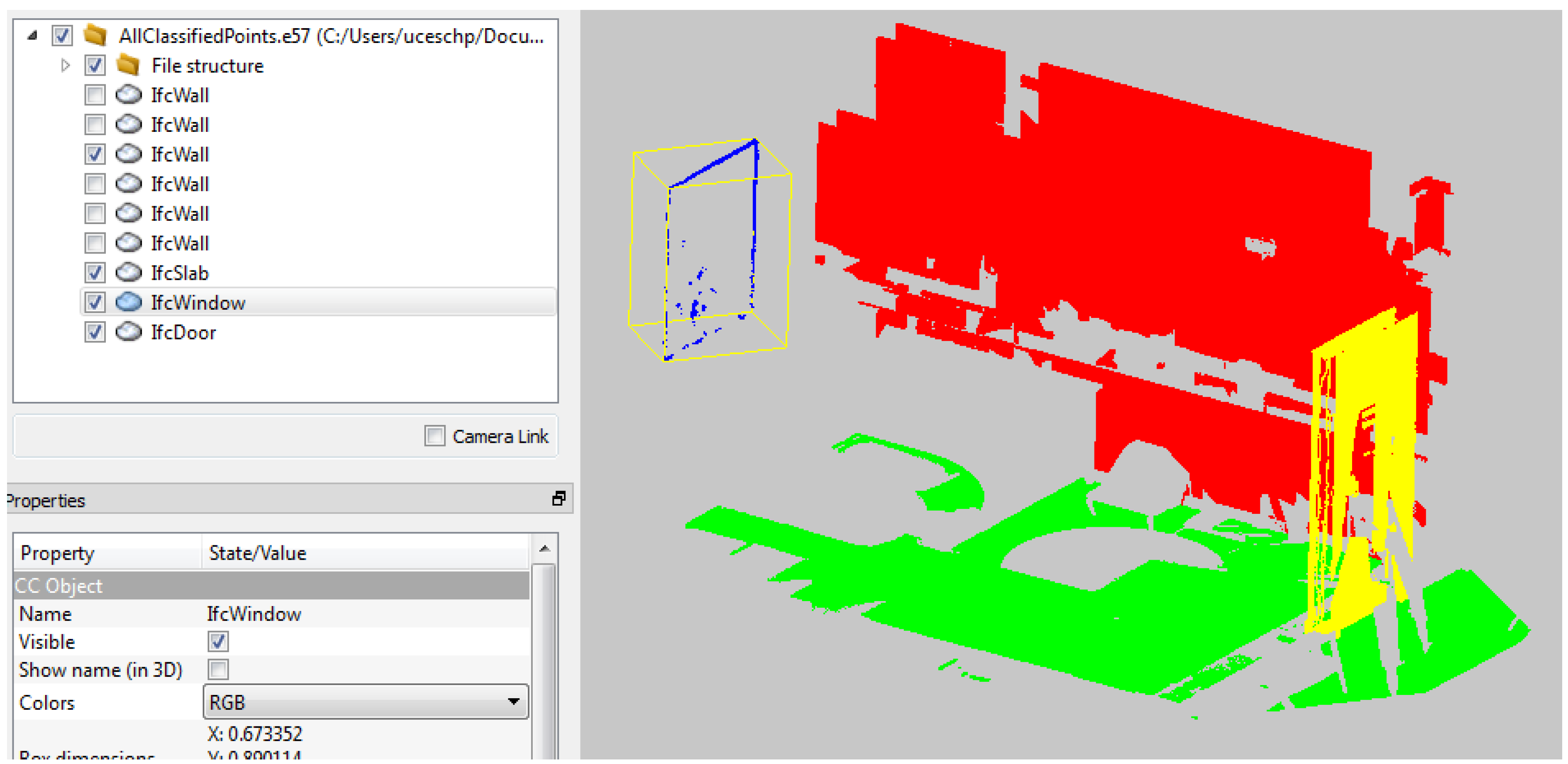
Once the bounding boxes are known, we can then extract the points within each box and colour them by type. This is performed with a 3D convex hull of the box which is then used to filter the dataset. Then, each segment can be written into the same E57 file as separate “scans” within the structure, each named after the IFC object they represent (Figure 4).
Figure 4.
E57 point cloud with each element classified by IFC type (loaded in CloudCompare with four of nine elements visible).
Figure 4.
E57 point cloud with each element classified by IFC type (loaded in CloudCompare with four of nine elements visible).

3. Findings
3.1. Data
The following is a brief outline of the data used to test the methods developed in this paper. A fuller description for the dataset that forms a benchmark for indoor modelling can be found in [47]. The dataset is freely available to download at: http://indoor-bench.github.io/indoor-bench. The datasets used are both sections of the Chadwick Building at UCL, each captured with state of the art methods of static and mobile laser scanning and accompanied by a manually created IFC model. This represents a typical historical building in London that has had several retrofits over the years to provide various spaces for the changing nature of activities within the UCL department housed inside.
3.1.1. Basic Corridor
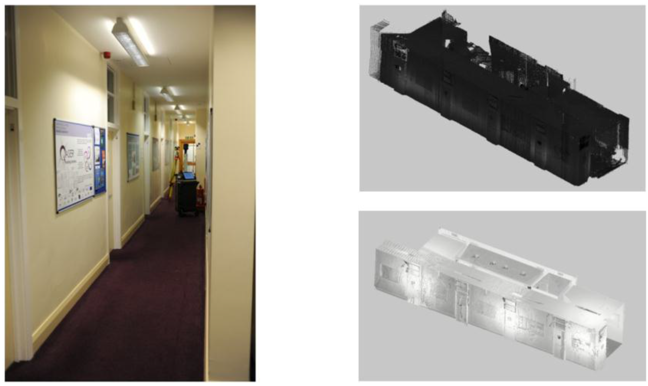
This first area is a long repetitive corridor section from the second floor of the building. It roughly measures 1.4 m wide by 13 m long with a floor to ceiling height of 3 m. The scene features doors off to offices at regular intervals and modern fluorescent strip lights standing proud of the ceiling as can be seen in Figure 5, along with the data captured with each instrument.
Figure 5.
Image of corridor (left) and resulting point cloud data collected with a Viametris Indoor Mobile Mapping System (top right) and Faro Focus 3D S (bottom right).
Figure 5.
Image of corridor (left) and resulting point cloud data collected with a Viametris Indoor Mobile Mapping System (top right) and Faro Focus 3D S (bottom right).

3.1.2. Cluttered Office
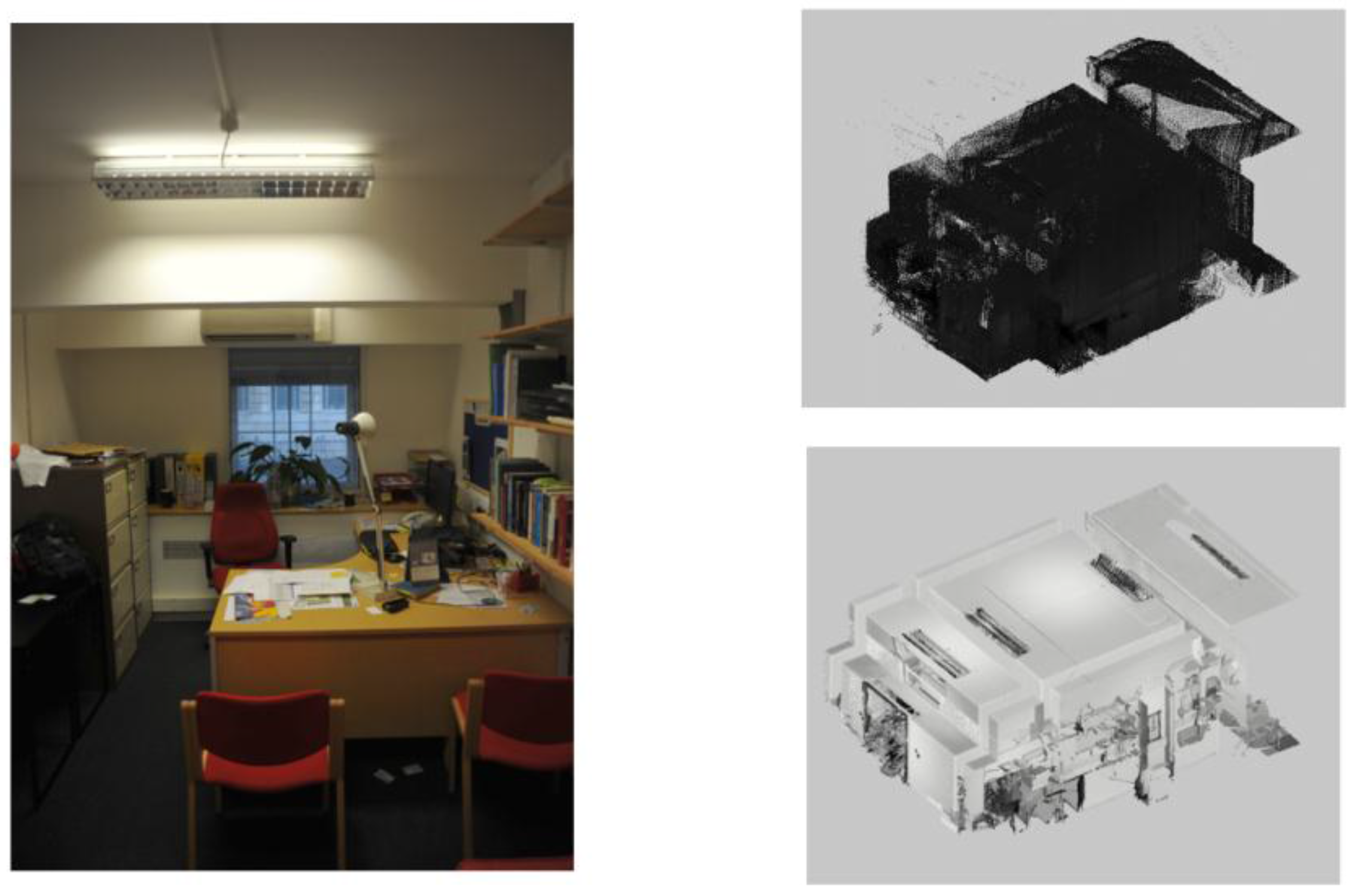
The second indoor environment is a standard office from the modern retrofitted mezzanine floor of the Chadwick Building. It roughly measures 5 m by 3 m with floor to ceiling height of 2.8 m at its highest point. The environment contains many items of clutter, which occlude the structural geometry of the room including filing cabinets, air conditioning unit, shelving, chairs and desks as illustrated in Figure 6, along with the data captured with each instrument.
Figure 6.
Image of office (left) and point cloud data collected with a Viametris Indoor Mobile Mapping System (top right) and Faro Focus 3D S (bottom right).
Figure 6.
Image of office (left) and point cloud data collected with a Viametris Indoor Mobile Mapping System (top right) and Faro Focus 3D S (bottom right).

3.2. Results
The data outlined in the previous section was fed into the point cloud to IFC algorithm described earlier in this paper and the results are presented here. The results from this process are split into those that are qualitative and can be observed in relation to the reference human-made model and more quantitative results that put figures to the deviations seen in the form of a quality metric that acts as a discrepancy measure between reference and test datasets.
3.2.1. Quality Metric
To compare the reconstructed geometry to the reference model the following is performed. For each wall in the reference model, the reconstructed test wall with the nearest centroid in 2D is transformed into the local coordinate space (as plotted in Figure 7) of the reference that then can be measured for geometric deviation in relation to this coordinate space.
This quality metric is composed of three criteria:
- the Euclidean distance offset between reference (indicated by subscript 1) and automated (indicated by subscript 2) wall centroids
- the area formed by the absolute difference in magnitude of the wall in width and length
- and the Sine of the angular difference
The distance d and the area A are normalised by dividing them by the maximum value. The quality metric is then computed by a weighted sum of the three normalised values
In other words, these values from formulas 1, 2, and 3 represent the quality of the global placement, the object construction and the angular discrepancy, respectively. All of these values indicate a better quality detection and therefore success of the fit when they tend to 0. The metric is a weighted sum where we currently choose all the weights wi to be 1/3 to keep the metric within the range 0-1. A value under 0.1 of this measure can be generally considered as very good. An alternative measure that gives similar relative results to this quality metric is the Hausdorff Distance. However, the ability to categorise the fit in our quality sum value by looking at the magnitude of the three components allows greater understanding and finer control through weighting than the measure provided by a Hausdorff Distance. The angular difference, for instance, could be more heavily weighted so that smaller angular changes have a greater impact on the final measure.
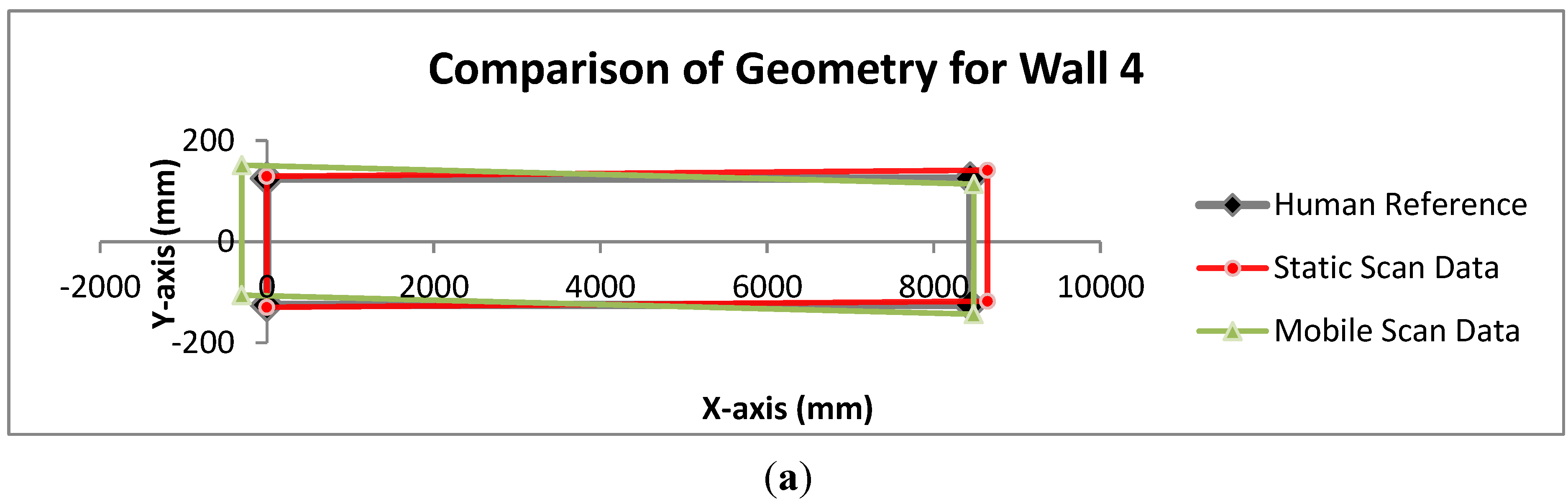
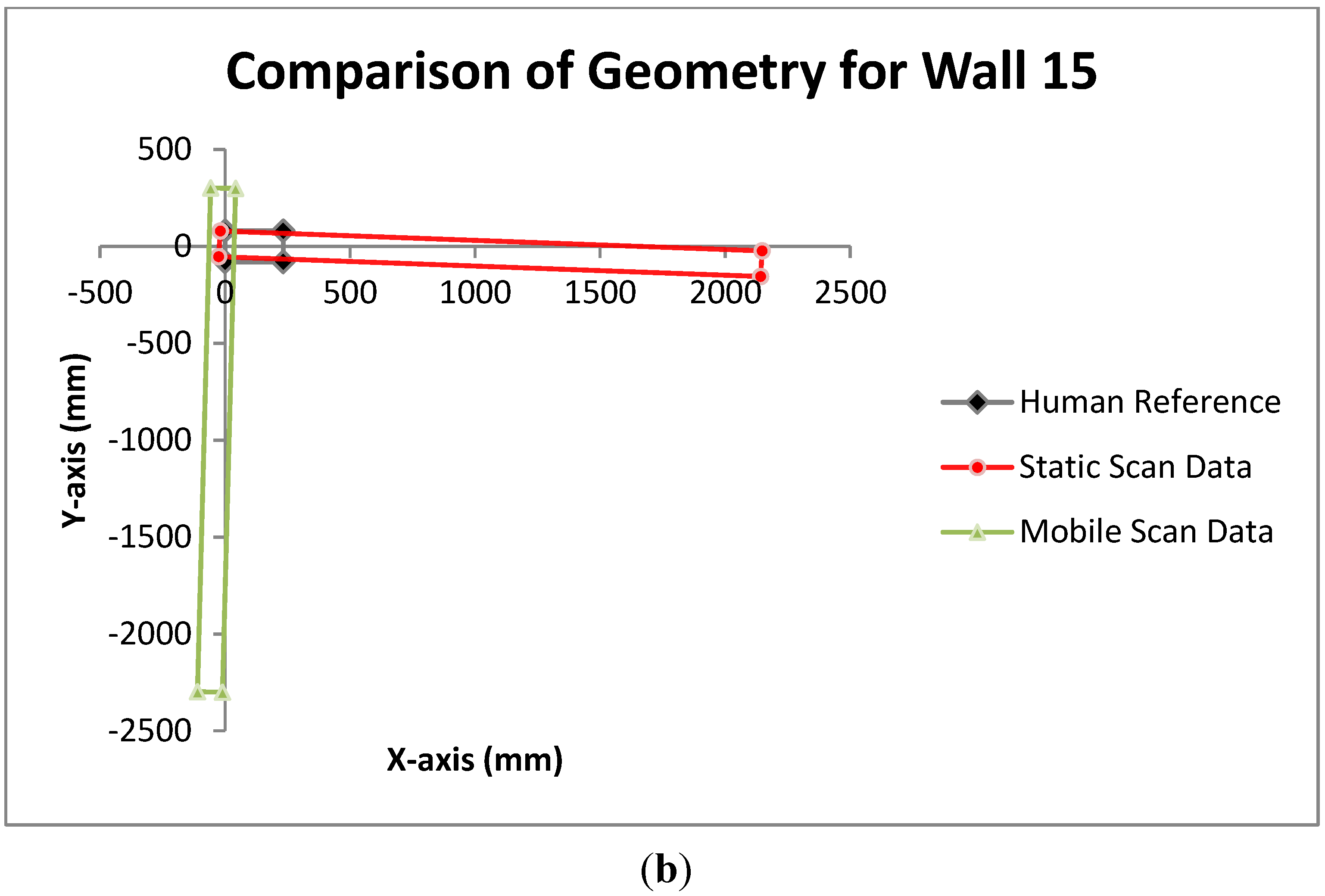
An example for the quality calculation using data comparing one of the corridor walls to the automatically extracted wall from static scan data is shown in Table 1 for a wall that is considered good by the quality metric and one that is considered almost ten times worse. To illustrate why these fits provide the quality values that they do, the wall geometries are plotted in Figure 7. The fit for wall 4, has been successfully recovered from both scan datasets looking at the plotted data, leading to good quality values, whereas wall 15 has a worse quality value by an order of magnitude as it is wrong in length by almost 2 m as illustrated in the plot. The value is low overall as its angular discrepancy is small against the reference, unlike wall 15 from the mobile data where the size and angle of the wall is wrong (Figure 7b) producing a larger quality value.

Table 1.
Example of data from a wall comparison with quality metric for a well (wall 4) and poorly (wall 15) reconstructed case of the corridor dataset against the static scan derived geometry.
| Delta Centroid X (mm) | Delta Centroid Y (mm) | Angular Difference (Deg) | Delta Wall Length (mm) | Delta Wall Width (mm) | Quality Metric | |
|---|---|---|---|---|---|---|
| Wall 4 | 102.9 | 5.8 | 179.9 | 209.6 | 249.6 | 0.029 |
| Wall 15 | 944.6 | 38.3 | 177.3 | 1935.7 | 153.8 | 0.233 |
Figure 7.
Plots of boundary placement of manual and automatically created geometry from the static scan data for (a) wall 4 and (b) wall 15 of the corridor dataset.
Figure 7.
Plots of boundary placement of manual and automatically created geometry from the static scan data for (a) wall 4 and (b) wall 15 of the corridor dataset.


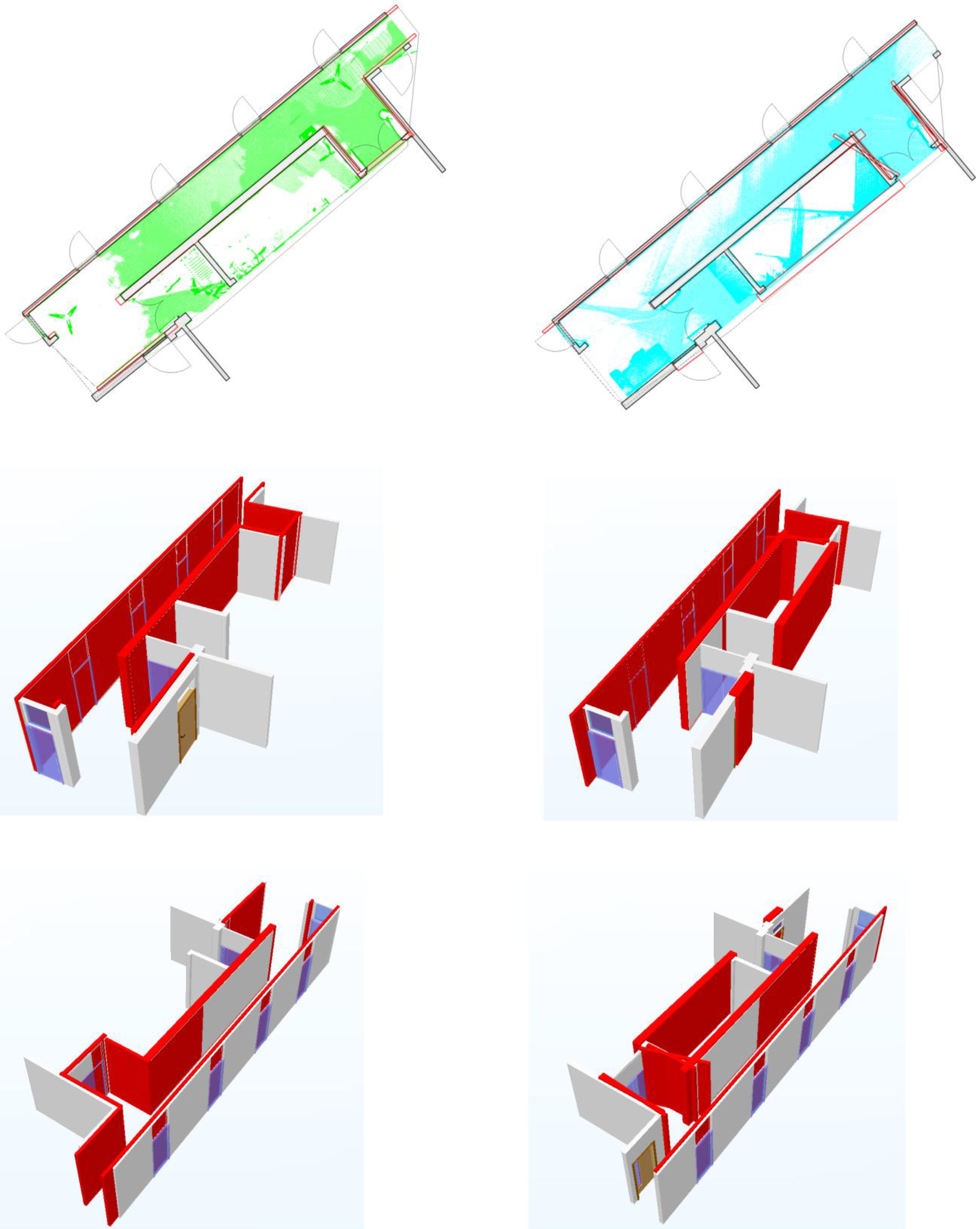
3.2.2. Point Cloud to IFC—Corridor
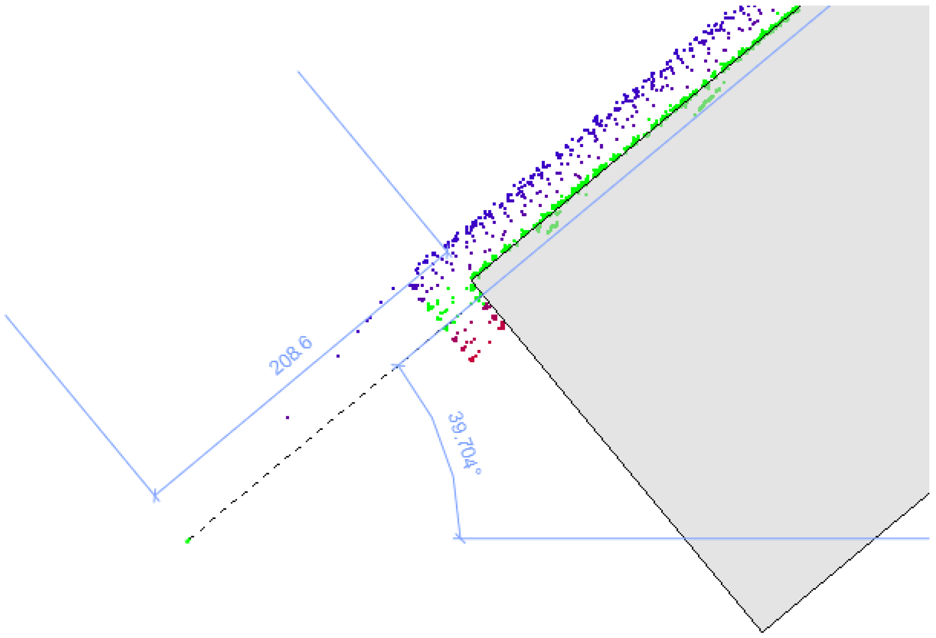
The majority of the space-bounding walls have been reconstructed as shown by Figure 8, with the central wall seeming to have the best construction from both static and mobile scan data. This is borne out by the quality measure (Figure 9) where this central wall (wall 4) scored the best. However, this wall does have a 200 mm over-extension in its reconstruction, representing an error of 2.3% of total length. This is due to extraneous noise outside the main wall affecting the maximum segment measurement for wall length extent as in Figure 10.
As edges are inferred as being the edge of the detected plane, then extraneous points from clutter or “split pixels” can affect the size of the recovered wall in the clustering stage as described above. Overall, the static scan data has allowed more walls to be recovered with greater confidence than the mobile data where the greater noise present in the data has created some ambiguity with multiple wall fits.
The spatial reasoning also appears to have been largely successful as all of the walls reconstructed from the static and a majority from the mobile data are actually walls in the reference with good approximations of width. The one wall from the mobile data that is incorrect runs along the Southeast edge of the plan view in Figure 8 and is caused by a planar façade to a long lectern that is geometrically close to a wall in planarity and point density. Figure 8 also shows that some of the walls detected from the static data have their normal pointing in the wrong direction leading to the wall lying on the wrong side of the wall surface found. This is a problem that is prevalent in almost every wall without a second side as there is no easy way to interpret the correct sidedness just from the geometry alone. This could be improved with geometric reasoning whereby the scan location is taken into account allowing ray casting to the points to attribute viewshed per location and therefore more robust normal prediction.
Figure 8.
Extracted walls (red) of the corridor from the static (green) and mobile (blue) point cloud data overlaid on the human-generated model (grey/white).
Figure 8.
Extracted walls (red) of the corridor from the static (green) and mobile (blue) point cloud data overlaid on the human-generated model (grey/white).

Table 2 provides some statistics about the walls that were well reconstructed from both sources of data. Length has generally been overestimated from both sets of data for the reasons described earlier with Figure 10. In the two components that are related to the walls’ width (delta of the centroid in Y and wall width itself) there is little difference between each dataset. This is to be hoped for, as the width/Y placement in local coordinates is dependent on the RANSAC plane found from the data. The error in wall width stems from the inability to estimate the wall width for two of the walls as only one side was scanned.
Table 2.
Statistics for the accuracy of the same reconstructed corridor walls considered good quality from both datasets (walls 3, 4 and 7) against the reference.
| Statistics for Good Quality Corridor Walls | Delta Centroid in X RMS (mm) | Delta Centroid in Y RMS (mm) | Angular Difference RMS (Deg.) | Delta Wall Length RMS (mm) | Delta Wall Width RMS (mm) |
|---|---|---|---|---|---|
| Static Scan Data | 180 | 43 | 0.20 | 371 | 186 |
| Mobile Scan Data | 256 | 45 | 0.50 | 401 | 186 |
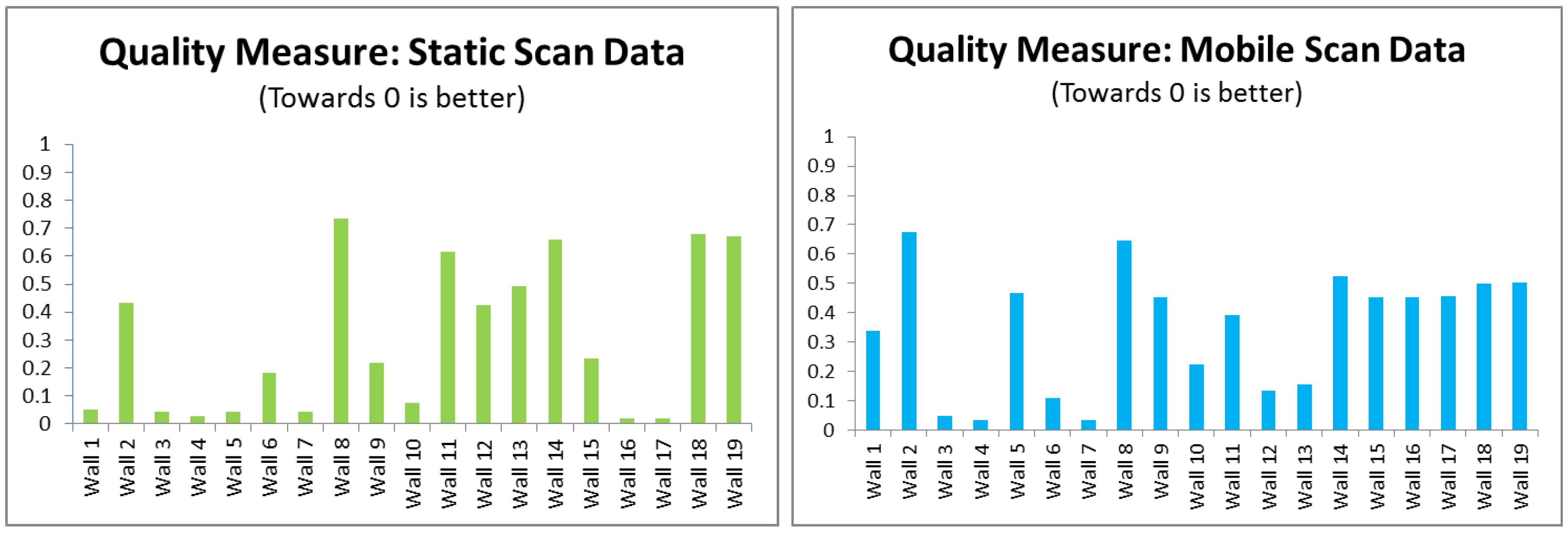
Figure 9.
Charts of calculated reconstruction quality for each wall in the reference human-created model of the corridor against the automated geometry from the two scan datasets.
Figure 9.
Charts of calculated reconstruction quality for each wall in the reference human-created model of the corridor against the automated geometry from the two scan datasets.

Figure 10.
Noise that caused over-extension from the static corridor scan data shown against reference wall.
Figure 10.
Noise that caused over-extension from the static corridor scan data shown against reference wall.

3.2.3. Point Cloud to IFC—Office
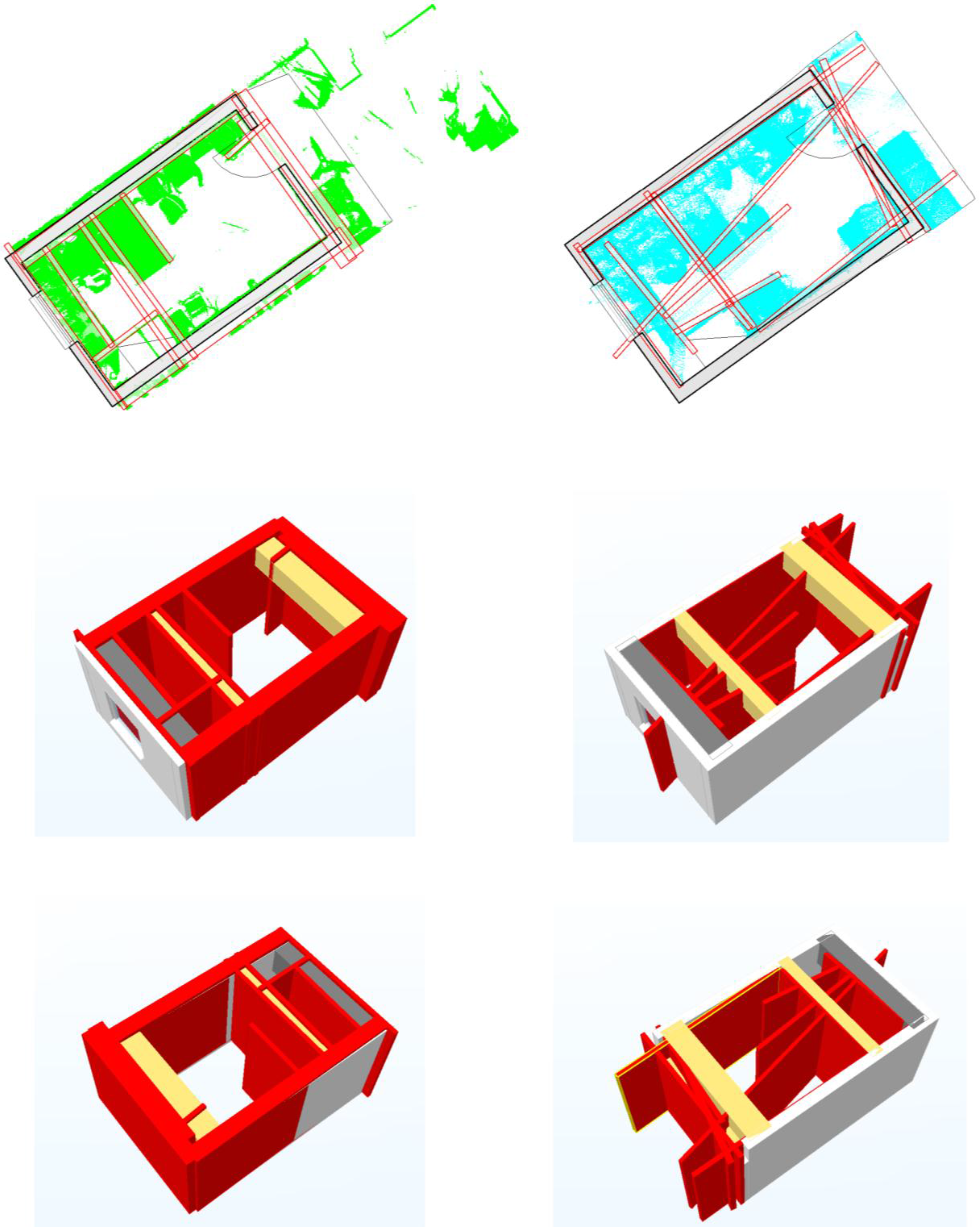
The main bounding walls of the office have been reconstructed with varying degrees of success. To aid with the description, starting at the wall with the door (Figure 11), the wall numbers going clockwise are 5, 4, 6, and 3. Walls 1 and 2 in the reference model are small height walls from the ceiling and floor respectively and can be seen at the end of the room above and below the window in Figure 6.
The geometry for walls 3 and 4, which have both sides captured in the static data, seems fairly good with an over-estimation of thickness due to the clutter present on those walls of the office. Wall 6 in the same data is well placed but with no backside scan data its width is incorrect, whereas in wall 5 the open door and chairs close to the outside face of the wall have affected the reconstruction. The extraneous walls from the clutter have survived due to their size being above the small wall limit, so the desk and filing cabinets are considered by the reasoning as partial walls, which is too simplistic, although correct for the first wall parallel to the window. A change to the algorithm to take the space of the room into account, e.g., maximum bounded area, may be a quick way to remove these surviving “walls” from clutter.
Figure 11.
Extracted walls (red) of the office from the static (green) and mobile (blue) point cloud data overlaid on the human-generated model (grey/white).
Figure 11.
Extracted walls (red) of the office from the static (green) and mobile (blue) point cloud data overlaid on the human-generated model (grey/white).

The mobile scan data does not have the second side to most of the walls in the data meaning that the thicknesses could not be estimated; the exception being wall 5 where the same problems that affected the static data reconstruction appear here. However, fewer of the elements of clutter have been turned into extraneous walls, probably due to the lower resolution of the objects and higher noise level of the mobile point cloud. The fact that the door has led to a plane being successfully fitted through the whole office would suggest that the threshold values for the Euclidean Clustering were too high for data from this sensor.
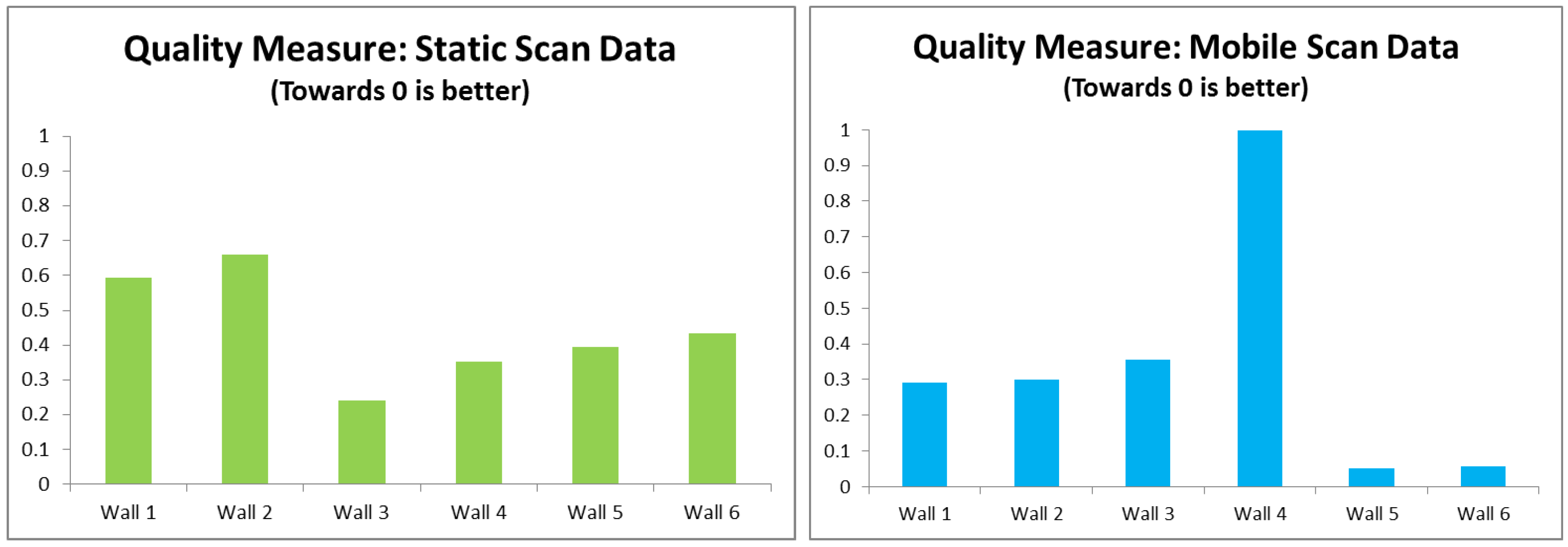
The chart of the static quality scores shows a fairly even level of quality with wall 3 being “best”; Figure 11 shows it as the wall with the least incorrect estimation in both width and length so seems valid. By looking at the results of the quality metric in Figure 12, the patchiness of the reconstruction can be seen. The figure for the mobile data shows a gross error for wall 4, which has depressed the quality values for walls 5 and 6 more than their visual placement would imply would be acceptable as such a good quality fit.
Looking at the statistical data for the reconstruction of bounding walls that were not failed reconstructions as shown in Table 3, the trend is much the same as the data from the corridor test. The wall width RMS values are similar between datasets with the length having quite large RMS values from the mobile scan data. The width is for similar reasons highlighted in the same section for the corridor data, namely the inability to guess a wall thickness given one wall side captured. The length errors in this set appear mainly down to clutter and manifest more on one side of the wall from the mobile reconstruction as the centroid mean X coordinate is much larger. In addition, the higher noise from the mobile scanners tied with the greater clutter in the scene has increased the ambiguity in the detection leading to increased errors.
Figure 12.
Charts of calculated reconstruction quality for each wall in the reference human-created model of the office against the automated geometry from the two scan datasets.
Figure 12.
Charts of calculated reconstruction quality for each wall in the reference human-created model of the office against the automated geometry from the two scan datasets.

Table 3.
Statistics for the accuracy of three of the main four bounding office walls from both datasets (walls 3, 5 and 6) against the reference model; wall 4 is ignored for the gross error from the mobile data detection as seen in Figure 12.
| Statistics for Good Quality Office Walls | Delta Centroid in X RMS (mm) | Delta Centroid in Y RMS (mm) | Angular Difference RMS (Deg.) | Delta Wall Length RMS (mm) | Delta Wall Width RMS (mm) |
|---|---|---|---|---|---|
| Static Scan Data | 159 | 101 | 0.47 | 539 | 204 |
| Mobile Scan Data | 378 | 100 | 0.45 | 602 | 206 |
4. Conclusions
The work presented in this paper has shown the applicability and limits to full automated reconstruction of object-based “intelligent” BIM geometry from point clouds in a format agnostic way. There has been partial success towards the aim of fully automatic reconstruction, especially where the environment is simple and not cluttered. Where both sides of a wall are present, the reconstruction has tended to be more reliable from both data sources. However, clutter, as is usual in the indoor environment, does have an effect. This was shown by the planar model presented here being supported by dense wall hosted or connected elements such as shelving or filing cabinets. A way to detect this data through more involved scene understanding would help. A method of doing this may be to take the intensity return or colour data present in the scans into account.
Clutter in the environment also has another effect and that is to hide or shadow the building features that need to be constructed. This is mitigated to a degree in the field by good survey design, but point clouds generated by imaging systems will, by their nature, suffer from occlusions somewhere in the dataset. This is something the routine presented here is affected by and unable to overcome in its current state e.g. if an alcove is hidden by an open door.
Computing power is an inherent problem when handling point cloud datasets and the approach presented here exacerbates it by relying on RAM for fast access to the whole dataset for processing. Downsampling is usually performed to keep the data manageable and could be applied in this case for very large datasets, however cloud computing presents a tangible opportunity to reduce the effect of this limitation by providing a scalable amount of computing power per process.
The data capture method does not seem to have a large bearing on the success of reconstruction except in the cluttered scene where the reduced resolution and more even sampling of the clutter objects in the mobile scan seems to prevent as many extraneous planes surviving the spatial reasoning step and affecting the geometry construction.
The question of what represents a good and bad reconstruction is crucial for comparisons and benchmarking. To provide a way of quantifying this, a quality measure has been developed based on the placement, size and angular discrepancies in relation to a reference model. This is not only useful for scoring automatically reconstructed geometry but could also prove useful when comparing an as-built model from scans against a base design model for verification throughout the construction phase of a project.
The logic required to make decisions about whether a certain geometry configuration is feasible already exists in commercial packages for design model verification (e.g. Solibri Model Checker [48]). It could easily be envisaged that this set of existing rules could be applied to automated models, as they are currently used to assess human-generated ones for building regulation infringements.
In terms of the scan-to-BIM workflow this work could be seen as a supplement to the semi-automatic construction of the bounding structural features of a building. For survey purposes the attribution of fit data is useful for quality assurance. Other stakeholders may require other semantic information that can be added to the IFC geometry created by this process or swapped out with more specific elements if required. Irregular and complex shapes require a more involved process and it will depend on fitness for purpose as to whether the recovery of an exact geometric description is worthwhile. Heritage and construction cases would tend to require this whereas simulation and operational management phases of BIM would accept a geometric generalisation.
Overall, the quality measure works well but the normalisation against a maximum value from the data means that the results from two different comparisons are not directly comparable, something that could be changed by setting the maximum limit to a threshold value after which values are set to 1.
Point clouds are now the basis for a large amount of 3D modelling of existing conditions and their importance has never been greater. However the complexity of effort to generate information for the BIM process is significant. Pure automation is currently not at a stage to be viable as the varied, cluttered nature of the indoor environment means that, currently, human intuition still triumphs over computerised methods alone. Ultimately the work presented in this paper is still best practically seen as an aid to a human user who can edit, accept or reject the geometry recovered by the algorithm in a semi-automated process.
Further Work
To continue this work, it would be beneficial to test the routine on larger datasets, such as one floor or many floors of a building as that would be a truer test of the algorithms main application. Further development of the process to take an IFC and classify a point cloud from it would help reverse the idea of a point cloud as being geometrically rich but information poor, bringing more value to the point cloud as a dataset.
Certain steps of the algorithm can also be refined. Generally refining the algorithm so that it is not so influenced by clutter would be beneficial. Linked to that is adding topological links so that walls that are close together can be joined, then logical building rules could be better applied (e.g., about bounded room volumes) and it would help to mitigate any incorrect determination of length from noise. The quality measure could also be refined by investigating weighting the three components differently or thresholding the normalisation so that a quality value from one comparison is equal to the same value from another set of data.
Acknowledgments
The authors would like to thank the reviewers and copy editors, whose helpful comments led to a better paper overall.
Author Contributions
Charles Thomson designed, executed and performed the analysis of the work presented in this paper as well as wrote the article with the guidance of Jan Boehm throughout the process.
Conflicts of Interest
The authors declare no conflict of interest.
References
- Pottmann, H. Geometry of architectural freeform structures. Proceedings of the 2008 ACM Symposium on Solid and Physical Modeling—SPM ’08; ACM Press: New York, NY, USA, 2008; Volume 209, p. 9. Available online: http://portal.acm.org/citation.cfm?doid=1364901.1364903 (accessed on 2 July 2015).
- Cabinet Office. Government Construction Strategy; London, UK, 2011. Available online: https://www.gov.uk/government/uploads/system/uploads/attachment_data/file/61152/Government-Construction-Strategy_0.pdf (accessed on 10 April 2012).
- UK Green Building Council. Retrofit. Available online: http://www.ukgbc.org/content/retrofit (accessed on 20 April 2013).
- U.S. General Services Administration. GSA BIM Guide for 3D Imaging; Washington, DC, USA, 2009. Available online: http://www.gsa.gov/graphics/pbs/GSA_BIM_Guide_Series_03.pdf (accessed on 10 April 2012).
- BIM Task Group. Work-streams and Work-packages. Available online: http://www.bimtaskgroup.org/work-streams-wps/ (accessed on 25 October 2012).
- Li, S.; Isele, J.; Bretthauer, G. Proposed methodology for generation of building information model with laserscanning. Tsinghua Sci. Technol. 2008, 13, 138–144. [Google Scholar] [CrossRef]
- Runne, H.; Niemeier, W.; Kern, F. Application of laser scanners to determine the geometry of buildings. In Optical 3D Measurement Techniques V; Grün, A., Kahmen, H., Eds.; Department of Applied and Engineering Geodesy, Institute of Geodesy and Geophysics, Vienna University of Technology: Vienna, Austria, 2001; pp. 41–48. [Google Scholar]
- Haala, N.; Anders, K. Fusion Of 2D-GIS and image data for 3D building reconstruction. Int. Arch. Photogram. Remote Sens. 1996, 31, 285–290. [Google Scholar]
- Suveg, I.; Vosselman, G. Reconstruction of 3D building models from aerial images and maps. ISPRS J. Photogramm. Remote Sens. 2004, 58, 202–224. [Google Scholar] [CrossRef]
- Chapman, D.P.; Deacon, A.T. D.; Hamid, A. HAZMAP: A remote digital measurement system for work in hazardous environments. Photogramm. Rec. 1994, 14, 747–758. [Google Scholar] [CrossRef]
- Rajala, M.; Penttilä, H. Testing 3D building modelling framework in building renovation. Communicating space(s), Proceedings of the 24th Education and Research in Computer Aided Architectural Design in Europe Conference; Bourdakis, V., Charitos, D., Eds.; University of Thessaly: Volos, Greece, 2006; pp. 268–275. Available online: http://www.mittaviiva.fi/hannu/studies/2006_rajal_penttila.pdf (accessed on 3 June 2013).
- Royal Institution of Chartered Surveyors. Scale; London, UK, 2010. Available online: http://www.rics.org/uk/knowledge/more-services/guides-advice/rics-geomatics-client-guide-series/ (accessed on 24 April 2014).
- Royal Institution of Chartered Surveyors. Measured Surveys of Land, Buildings and Utilities; London, UK, 2014, 3rd ed. Available online: http://www.rics.org/uk/knowledge/professional-guidance/guidance-notes/measured-surveys-of-land-buildings-and-utilities-3rd-edition/ (accessed on 24 April 2014).
- Plowman Craven Limited. PCL BIM Survey Specification v2.0.3; Harpenden, UK, 2012. Available online: http://www.plowmancraven.co.uk/bim-survey-specification/ (accessed on 26 April 2014).
- Larsen, K.E.; Lattke, F.; Ott, S.; Winter, S. Surveying and digital workflow in energy performance retrofit projects using prefabricated elements. Autom. Constr. 2011, 20, 999–1011. [Google Scholar] [CrossRef]
- Day, M. Scan-to-BIM: A reality check. Available online: http://aecmag.com/index.php?option=content&task=view&id=498 (accessed on 25 May 2013).
- Eastman, C.M.; Teicholz, P.; Sacks, R.; Liston, K. BIM Handbook: A Guide to Building Information Modeling for Owners, Managers, Designers, Engineers and Contractors, 2nd ed.; John Wiley and Sons: Hoboken, NJ, USA, 2011. [Google Scholar]
- Tang, P.; Huber, D.; Akinci, B.; Lipman, R.; Lytle, A. Automatic reconstruction of as-built building information models from laser-scanned point clouds: A review of related techniques. Autom. Constr. 2010, 19, 829–843. [Google Scholar] [CrossRef]
- Pu, S.; Vosselman, G. Automatic extraction of building features from terrestrial laser scanning. Int. Arch. Photogramm. Remote Sens. Spat. Inf. Sci. 2006, 36, 25–27. [Google Scholar]
- Tao, C.V. 3D data acquision and object reconstruction for AEC/CAD. In Large-scale 3D Data Integration: Challenges and Opportunities; Zlatanova, S., Prosperi, D., Eds.; CRC Press: Boca Raton, FL, USA, 2005; pp. 39–56. [Google Scholar]
- Hichri, N.; Stefani, C.; De Luca, L.; Veron, P. Review of the « As-Built BIM » approaches. Int. Arch. Photogramm. Remote Sens. Spat. Inf. Sci. 2013, XL-5/W1, 107–112. [Google Scholar] [CrossRef]
- Müller, P.; Wonka, P.; Haegler, S.; Ulmer, A.; Van Gool, L. Procedural Modeling of Buildings; ACM Press: New York, NY, USA, 2006. [Google Scholar] [CrossRef]
- Kelly, G.; McCabe, H. A survey of procedural techniques for city generation. ITB J. 2006, 14, 87–130. [Google Scholar]
- Khoshelham, K.; Díaz-Vilariño, L. 3D Modelling of interior spaces: Learning the language of indoor architecture. ISPRS Int. Arch. Photogramm. Remote Sens. Spat. Inf. Sci. 2014, XL-5, 321–326. [Google Scholar] [CrossRef]
- Besl, P.J.; Jain, R.C. Three-dimensional object recognition. ACM Comput. Surv. 1985, 17, 75–145. [Google Scholar] [CrossRef]
- Barnea, S.; Filin, S. Segmentation of terrestrial laser scanning data using geometry and image information. ISPRS J. Photogramm. Remote Sens. 2013, 76, 33–48. [Google Scholar] [CrossRef]
- Budroni, A.; Boehm, J. Automated 3D reconstruction of interiors from point clouds. Int. J. Archit. Comput. 2010, 8, 55–73. [Google Scholar] [CrossRef]
- Adan, A.; Huber, D. 3D reconstruction of interior wall surfaces under occlusion and clutter. In Proceedings of the IEEE International Conference on 3D Imaging, Modeling, Processing, Visualization and Transmission (3DIMPVT), Hangzhou, China, 16–19 May 2011; pp. 275–281.
- Hoover, A.; Jean-Baptiste, G.; Jiang, X.; Flynn, P.J.; Bunke, H.; Goldgof, D.B.; Bowyer, K.; Eggert, D.W.; Fitzgibbon, A.; Fisher, R.B. An experimental comparison of range image segmentation algorithms. IEEE Trans. Pattern Anal. Mach. Intell. 1996, 18, 673–689. [Google Scholar] [CrossRef]
- Xiong, X.; Adan, A.; Akinci, B.; Huber, D. Automatic creation of semantically rich 3D building models from laser scanner data. Autom. Constr. 2013, 31, 325–337. [Google Scholar] [CrossRef]
- Jung, J.; Hong, S.; Jeong, S.; Kim, S.; Cho, H.; Hong, S.; Heo, J. Productive modeling for development of as-built BIM of existing indoor structures. Autom. Constr. 2014, 42, 68–77. [Google Scholar] [CrossRef]
- Volk, R.; Stengel, J.; Schultmann, F. Building Information Modeling (BIM) for existing buildings—Literature review and future needs. Autom. Constr. 2014, 38, 109–127. [Google Scholar] [CrossRef]
- Nagel, C.; Stadler, A.; Kolbe, T.H. Conceptual requirements for the automatic reconstruction of building information from uninterpreted 3D models. In GeoWeb 2009 Academic Track - Cityscapes; Kolbe, T.H., Zhang, H., Zlatanova, S., Eds.; ISPRS: Vancouver, BC, Canada, 2009; Volume 38, pp. 46–53. [Google Scholar]
- ClearEdge3D. Edgewise Building. Available online: http://www.clearedge3d.com/products/edgewise-building/ (accessed on 9 June 2015).
- IMAGINiT Technologies. Scan to BIM. Available online: http://www.imaginit.com/software/imaginit-utilities-other-products/scan-to-bim (accessed on 19 June 2015).
- Faro 3D Software GmBH. Software for Surveying and As-Built Documentation. Available online: http://faro-3d-software.com/index.php (accessed on 9 June 2015).
- Pointcab. Point Cloud Processing Software. Available online: http://www.pointcab-software.com/en/ (accessed on 9 June 2015).
- BuildingSMART International. IFC Overview Summary. Available online: http://www.buildingsmart-tech.org/specifications/ifc-overview/ifc-overview-summary (accessed on 4 December 2012).
- Bonsma, P.P. Basic IFC knowledge. Available online: http://www.buildingsmart-tech.org/implementation/ifc4-implementation/basic-ifc-knowledge (accessed on 7 Feburary 2013).
- Rusu, R.B.; Cousins, S. 3D is here: Point Cloud Library (PCL). In Proceedings of the IEEE International Conference on Robotics and Automation, Shanghai, China, 9–13 May 2011; pp. 1–4.
- Ward, A.; Benghi, C.; Ee, S.; Lockley, S. The eXtensible Building Information Modelling (xBIM) Toolkit. Available online: http://nrl.northumbria.ac.uk/13123/ (accessed on 20 Feburary 2015).
- E57.04 3D Imaging System File Format Committee. libE57: Software Tools for Managing E57 files (ASTM E2807 standard). Available online: http://www.libe57.org/ (accessed on 20 Feburary 2015).
- Fischler, M.A.; Bolles, R.C. Random sample consensus: A paradigm for model fitting with applications to image analysis and automated cartography. Commun. ACM 1981, 24, 381–395. [Google Scholar] [CrossRef]
- Monszpart, A.; Mellado, N.; Brostow, G.J.; Mitra, N.J. RAPTER: Rebuilding Man-made Scenes with regular arrangements of planes: SIGGRAPH 2015. Available online: http://geometry.cs.ucl.ac.uk/projects/2015/regular-arrangements-of-planes/ (accessed on 18 June 2015).
- Rusu, R.B. Semantic 3D Object Maps for everyday manipulation in human living environments. KI—Künstliche Intell. 2010, 24, 345–348. [Google Scholar] [CrossRef]
- Liebich, T.; Adachi, Y.; Forester, J.; Hyvarinen, J.; Karstila, K.; Reed, K.; Richter, S.; Wix, J. IFC2x Edition 3 Technical Corrigendum 1. 2007. Available online: http://www.buildingsmart-tech.org/ifc/IFC2x3/TC1/html/index.htm (accessed on 2 March 2015).
- Thomson, C.; Boehm, J. Indoor modelling benchmark for 3D geometry extraction. ISPRS Int. Arch. Photogramm. Remote Sens. Spat. Inf. Sci. 2014, XL-5, 581–587. [Google Scholar] [CrossRef]
- Solibri. Model Checker. Available online: http://www.solibri.com/products/solibri-model-checker/ (accessed on 20 June 2015).
© 2015 by the authors; licensee MDPI, Basel, Switzerland. This article is an open access article distributed under the terms and conditions of the Creative Commons Attribution license (http://creativecommons.org/licenses/by/4.0/).
Share and Cite
MDPI and ACS Style
Thomson, C.; Boehm, J. Automatic Geometry Generation from Point Clouds for BIM. Remote Sens. 2015, 7, 11753-11775. https://doi.org/10.3390/rs70911753
AMA Style
Thomson C, Boehm J. Automatic Geometry Generation from Point Clouds for BIM. Remote Sensing. 2015; 7(9):11753-11775. https://doi.org/10.3390/rs70911753
Chicago/Turabian StyleThomson, Charles, and Jan Boehm. 2015. "Automatic Geometry Generation from Point Clouds for BIM" Remote Sensing 7, no. 9: 11753-11775. https://doi.org/10.3390/rs70911753