Identification of Village Building via Google Earth Images and Supervised Machine Learning Methods

Abstract

In this study, a method based on supervised machine learning is proposed to identify village buildings from open high-resolution remote sensing images. We select Google Earth (GE) RGB images to perform the classification in order to examine its suitability for village mapping, and investigate the feasibility of using machine learning methods to provide automatic classification in such fields. By analyzing the characteristics of GE images, we design different features on the basis of two kinds of supervised machine learning methods for classification: adaptive boosting (AdaBoost) and convolutional neural networks (CNN). To recognize village buildings via their color and texture information, the RGB color features and a large number of Haar-like features in a local window are utilized in the AdaBoost method; with multilayer trained networks based on gradient descent algorithms and back propagation, CNN perform the identification by mining deeper information from buildings and their neighborhood. Experimental results from the testing area at Savannakhet province in Laos show that our proposed AdaBoost method achieves an overall accuracy of 96.22% and the CNN method is also competitive with an overall accuracy of 96.30%.

1. Introduction

With the rapid development of urbanization processes, maps used to illustrate buildings and their distribution are significant and are required in a wide range of fields. Important applications include environmental monitoring, resource management, disaster response, and homeland security [1]. In urban areas, accurate maps are often available; however, this is not always the case for villages and there may be no digital version available, which has several negative consequences. For instance, during catastrophic events such as the Wenchuan earthquake in 2008, disaster relief could not be conveniently provided due to inadequate rural information and because the location of residential buildings was uncertain, which resulted in serious loss of life and property [2]. A swift update of building information is very important and essential during catastrophes [3] because secondary disasters such as tsunamis, avalanches, and landslides may follow [4], causing swift changes to land conditions. In rural planning, which aims to benefit the inhabitants, public facilities need to be developed on the basis of the residential buildings’ distribution information [5]. To solve such complicated problems, the tools used to identify buildings must provide rapid, accurate, efficient, and time-sequenced results.

With the help of remote sensing satellite images [6,7,8], earth-observation activities on regional to global scales can be implemented owing to advantages such as wide spatial coverage and high temporal resolution [9,10]. Most previous studies that focus on village mapping commonly use low- and medium-spatial resolution images such as Landsat Thematic Mapper (TM), The Enhanced Thematic Mapper Plus (ETM+), and National Oceanic and Atmospheric Administration (NOAA)/ Advanced Very High Resolution Radiometer (AVHRR) [11,12,13], whereas in recent years, high-resolution images such as QuickBird, Ikonos, and RapidEye facilitate high-accuracy identification. Unfortunately, considering the high cost of data acquisition, these high-resolution images are generally utilized in a specific small region and are rarely applied in large ones [14].

A promising alternative solution is offered by Google Earth (GE), which provides open, highly spatially resolved images suitable for village mapping [15,16,17,18]. However, GE images have rarely been used as the main data source in village mapping. GE images are limited to a three-band color code (R, G, and B), which is expected to lower the classification performance due to its poor spectral signature [19]. Actually, the potential for the classification of spatial characteristics by Google Maps has been underestimated [20]. By analyzing the tone, texture, and geometric features in a GE image [18,21], experts can recognize village buildings with high confidence. Consequently, we believe that GE images can provide a good data source for village mapping.

In terms of classification technique, many methods have been studied by consulting published literature. With the help of image processing and feature extraction techniques, various machine learning algorithms [22] in remote sensing have been implemented. The AdaBoost method [23] is widely used in remote sensing pattern recognition. For instance, Zhang et al. [24] combine the K-means method with AdaBoost to classify buildings, and the overall accuracy is about 90%. Zongur et al. [25] utilize satellite images to detect an airport runway using AdaBoost with a circular-Mellin feature. Using an improved Normalized Difference Build-up Index (NDBI) and remote sensing images, Li et al. [26] dynamically extract urban land. Cetin et al. [27] use textural features such as the mean and standard deviation of image intensity and gradient for building detection. In the field of remote sensing detection, using the convolutional neural networks (CNN) method [28], Chen et al. [29] address vehicle detection, Li et al. [30] focus on building pattern classifiers, and Yue et al. [31] use both spectral and spatial features for hyperspectral image classification. To predict geoinformative attributes from large-scale images, Lee et al. [32] also choose CNN, and Sermanet et al. [33] utilize the CNN method to identify house numbers. In high-resolution image processing, Hu et al. [34] solved scene classification tasks using CNN and achieved an overall accuracy of approximately 98%. Other machine learning methods such as support vector machines (SVM) [35], which maximizes the margin in high-dimensional feature spaces using kernel methods for the samples, are introduced for classification. For the identification of forested landslides, Dou et al. [36] utilize a case-based reasoning approach and Li et al. [37] adopt two machine learning algorithms: random forest (RF) and SVM. When dealing with classifying complex mountainous forests via remote sensing images, Attarchi et al. [38] verify the performances of three machine learning methods: SVM, neural networks (NN), and RF. For mapping urban areas of DMSP/OLS nighttime light and MODIS data, Jing et al. [39] also utilize SVM.

To investigate the accuracy and efficiency of identification considering the characteristics of GE images, we herein explore the feasibility of supervised machine learning approaches for building identification using AdaBoost and CNN, respectively. Both methods adopt different feature extraction schemes, enabling full exploitation of the texture, spectral, geometry, and other characteristics in the images. The AdaBoost algorithm focuses on the color and textural information of the buildings and their surrounding areas; hence, it utilizes both color information and a large number of Haar-like features.

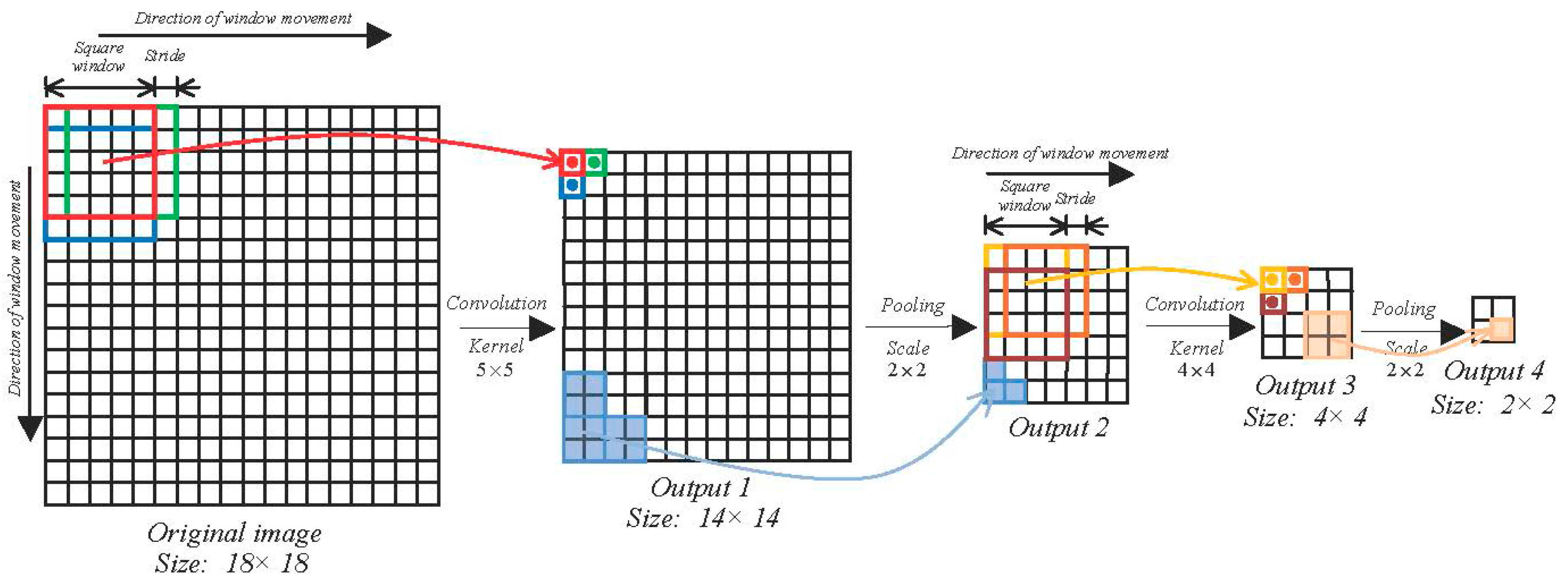
The performance of the AdaBoost method largely depends on the quality of the feature selection, which is itself quite challenging. In contrast, the CNN method achieves more robust and stronger performance than AdaBoost because it mines the deeper representative information from low-level inputs [28]. With multilayer networks trained by a gradient descent algorithm, CNN can learn complex and nonlinear mapping from a high- to low-dimensional feature space. Here, we constructed a four layer CNN network to describe the characteristics inside an 18 × 18-pixel window and applied it to the classification.

The remainder of our paper is organized as follows. In Section 2, we describe the study area and the experimental data. In Section 3, we briefly introduce the principles of the AdaBoost and CNN methods. We compare and analyze the experimental results of each algorithm in Section 4. The performance of our proposed method and suggestions for future work are presented in Section 5.

2. Study Area and Data

2.1. Study Area

In contrast to densely packed urban buildings, village buildings tend to be sparsely scattered. In this study, we define “village buildings” as any settlement with size less than 2 km. The study area, Kaysone (Figure 1a), is located at the Savannakhet province (Figure 1b) in Laos. The remote top-view RGB image of Kaysone has a size of 3600 × 4500 pixels with a resolution of 1 m, which was captured from Google’s satellite map in February 2015. Its longitude and latitude range from E104°47′22″ to E104°49′54″ and from N16°34′28″ to N16°36′26″, respectively, showing an area of approximately 19.44 km². The projection is in the UTM Zone 48N system and Datum WGS 84. The study area is a complex and rural region with many different types of landscape, including natural components such as mountains, rivers, and vegetation cover as well as artificial areas such as villages, roads, and cultivated land, which are typical in rural areas.

2.2. Data

As the training dataset, we selected four typical village/non-village areas (see Figure 1) from the original image. Each image was sized 600 × 900 pixels. Figure 1c,d in rich in village information, showing features such as buildings, roads, rivers, and cultivated lands. Figure 1f contains forests and mountains, whereas Figure 1e features crop and vegetation cover. The test data are contained within the entire area of Figure 1a. Within this area, the ground truth map of the village buildings was manually drawn beforehand using a polygon-based interaction tool. This ground truth map contains accurate information of the land categories and is chiefly used in sampling and result detection.

3. Machine Learning Approaches

Machine learning approaches can be divided into two broad categories: supervised and unsupervised. In general, unsupervised learning methods cannot learn the characteristics of GE images to a satisfactory level because of their limited distinguishability and lack of prior knowledge. Supported by training data, supervised learning methods usually deliver better classification results. In this study, AdaBoost and CNN were employed as classifiers and the feature extraction step was designed accordingly. Another popular alternative is SVM, which effectively solves nonlinear and higher dimensional problems [40]. However, in preliminary tests , SVM delivered similar performance to AdaBoost and required much longer computational time. Therefore, we exclude the SVM method in the present analysis.

3.1. AdaBoost Algorithm

The AdaBoost classification method [23,41] has gained great popularity due to its high accuracy, low complexity, and ability to recognize salient features. Based on the sample data, this algorithm iteratively adjusts the weights of many weak classifiers and builds these weak classifiers into a strong classifier. The samples are defined as:

$$(x_1,y_1),\mathrm{...},(x_m,y_m)$$

(1)

where $m$ refers to the number of samples, and $x_i\in X,y_i\in Y=\{-1,+1\}$. Note the inclusion of both positive and negative input samples. Initially, all samples are equally weighted as follows:

$$W_1(x_i)=1/m$$

(2)

The weight is adjusted after checking the performance of the weak classifier. If a sample cannot be correctly classified, its weight is increased. The details of the AdaBoost algorithm are shown below:

For $t=1,\mathrm{...},T$:

Train weak learner using distribution $W_t$.

• Get weak hypothesis $h_t:X\to \{-1,+1\}$, with error:

  $${\epsilon }_t=\text{Pr}\left[h_t(x_i)\ne y_i\right]$$

  (3)
• Choose:

  $${\alpha }_t=\frac{1}{2}ln\left(\frac{1-{\epsilon }_t}{{\epsilon }_t}\right)$$

  (4)
• Update:

  $$\begin{array}{c}{W}_{t+1}\left(x_i\right)=\frac{W_t(x_i)}{Z_t}\times \{\begin{array}{ll}{e}^{-{\alpha }_t}& \text{if }{h}_t(x_i)=y_i\\ e^{{\alpha }_t}& \text{if }{h}_t(x_i)\ne y_i\end{array}\\ =\frac{W_t(x_i)\text{exp}\left(-{\alpha }_t{y}_i{h}_t(x_i)\right)}{Z_t}\end{array}$$

  (5)

  where T is the total number of weak classifiers and $Z_t$ is a normalization factor, which is chosen such that $W_{t+1}$ is a distribution.

Output the final hypothesis:

$$H\left(x\right)=sign\left({\displaystyle \sum _{t=1}^T{\alpha }_t{h}_t(x)}\right)$$

(6)

where ${\alpha }_t$ indicates the weight of a weak classifier $h_t$. If ${\alpha }_t$ is large, the corresponding weak classifier plays an important role in the final combination, indicating a relatively the important feature.

Manually extracting the relevant features of village buildings is a challenging task. To improve the classification accuracy, the AdaBoost algorithm instead constructs the weak classifiers from a large number of simple features. Meanwhile, although the input dimension is quite high, the AdaBoost algorithm is robust to over-fitting problems [42]. In our experiment, we automatically generated 500 weak classifiers by applying the sample data to a three-layer decision tree.

3.1.1. Color Feature

To optimize the classifier for detecting the characteristics of color-coded GE images, we utilized four kinds of input samples from the images in Figure 1, varying the window size from 1 × 1 to 7 × 7 pixels to show the color information of specific blocks. Given an m × n sized color image patch, AdaBoost organizes the color feature by reshaping the color of each pixel in the patch into an m × n × 3 vector.

3.1.2. Haar-Like Feature

Haar-like features are proven to be efficient tools for detecting textural and structural information of buildings [23]. In this study, a large number of Haar-like features are generated for classification. By considering not only the target pixel but also the pixels inside its neighborhood window, the texture and structural characteristics of buildings can be well recognized.

The Haar-like features were generated by adopting several basic Haar filters and shifting and scaling them inside the neighborhood window. Figure 2 demonstrates the application of a 2 × 1 Haar filter. Here, w and h denote the width and height of the filter, respectively. The original filter is presented in Figure 2a. Shifting this filter inside the window, we obtain the various features shown in Figure 2b. Similarly, some results of shifting and scaling operations are presented in Figure 2c,d. In these panels, the original filter was enlarged to 4 × 2 and 6 × 3, respectively.

3.2. Convolutional Neural Networks (CNN)

CNN was inspired by biological entities. When multilayer networks are trained with gradient descent algorithms, they can learn complex nonlinear mappings from a high- to a low-dimensional feature space, where classification is evident [43]. Importantly, the simplified low-dimensional space can largely restore the information of the high-dimensional features, and it mines deeper information of the input high-dimensional features. CNN vertically concatenates an m × n RGB image patch into a 3m × n matrix. Here, we briefly introduce the framework of CNN; the details are provided in [28,43]. In implementing CNN, we utilized the DeepLearnToolbox library developed by [44].

To simplify the high-dimensional feature, the approach utilizes a multilayer system, including convolution and subsampling layers, as shown in Figure 3. Convolution can enhance the raw signal while decreasing the noise signal; the subsampling layer can utilize the correlation of the contiguous pixels, pooling the feature into lower dimensions without losing meaningful information. With the increase of layers, the dimension decreases but the number of features increases.

To restore the information of high-dimensional features to the greatest extent, the key point is back propagation. Similar to neural networks, to connect layers $i$ and $j$, one important parameter is the propagation weight $W_{ij}$, and another is the bias $b_i$. At the beginning, $W_{ij}$ and $b_i$ are randomly decided as 0. Then, we perform step-forward propagation

$$z^{(l+1)}=W^{(l)}{a}^{(l)}+b^{(l)}$$

(7)

$$a^{(l+1)}=f\left(z^{\left(l+1\right)}\right)$$

(8)

where $z^l$ denotes the total weighted sum of inputs to all the units in layer $l$, $f(x)$ is the activation function, such as a sigmoid, $a^l$ denotes the activation (meaning output value) of all the units in layer $l$. After the iteration, output $h_{W,b}(x)$ is produced. Due to the primitive definition of $W_{ij}^{}$ and $b_i$, there must be some error between the result and the true value. Two kinds of error are important, which can measure the accuracy of the network.

$${\delta }_i^{\left(l\right)}=\left({\displaystyle \sum _{j=1}^{s_{l+1\_}}{W}_{ji}^{(l)}}-{\delta }_j^{(l+1)}\right)f’\left(z_i^{(l)}\right)$$

(9)

$${\delta }_i^{\left(n_l\right)}=\frac{\partial }{\partial z_i^{\left(n_t\right)}}\frac{1}{2}{\Vert y-h_{W,b}(x)\Vert }^2=-\left(y_i-a_i^{(n_l)}\right)\cdot f’\left(z_i^{(n_t)}\right)$$

(10)

where ${\delta }_i^{\left(l\right)}$ refers to the error in each output unit $i$ in each layer $l$; it measures how far the corresponding node is responsible for any error in the output. ${\delta }_i^{\left(n_l\right)}$ denotes the error for each output unit $i$ in the output layer $n_l$. In addition to the error to get the optimum solution of $W_{ij}$ and $b_i$, we utilize an efficient iteration algorithm called a gradient descent,

$$W_{ij}^{\left(l\right)}=W_{ij}^{\left(l\right)}-\alpha \frac{\partial }{\partial W_{ij}^{(l)}}J\left(W,b\right)$$

(11)

$$b_i^{(l)}=b_i^{(l)}-\alpha \frac{\partial }{\partial b_i^{(l)}}J\left(W,b\right)$$

(12)

where $\alpha$ is the learning rate and the definition of $J(W,b)$ is an average sum-of-squares error term. We can efficiently compute the solution of the partial derivatives using back propagation. Incorporating ${\delta }_i^{\left(n_l\right)}$ and ${\delta }_i^{\left(l\right)}$, we can get

$$\frac{\partial }{\partial W_{ij}^{(l)}}J\left(W,b\right)=a_j^{(l)}{\delta }_i^{(l+1)}$$

(13)

$$\frac{\partial }{\partial b_i^{(l)}}J\left(W,b\right)={\delta }_i^{(l+1)}$$

(14)

After the iteration, $W_{ij}$ and $b_i$ are updated into the optimum solution; then we can calculate the optimum classification $h_{W,b}(x)$.

Based on the multilayer networks, the parameters of convolution subsampling cores are significant. In our experiment, the sequence of middle layers contains four layers $C_1$, $S_1$, $C_2$, and $S_2$. The data of each layer set is shown in

Table 1. Input data of middle layers.

Core	Output Maps	Kernel Size	Pooling Scale
Convolution 1	6	5	-
Subsampling 2	-	-	2
Convolution 3	12	4	-
Subsampling 4	-	-	2

, and the concrete process is shown in Figure 3.

Both the kernel size and pooling scale can turn the sample from a high- to low-dimensional feature space. As set initially, the size of the sample window is 18 × 18 in 3D; after going through the convolution for the first time, the size changes to 14 × 14, which becomes 7 × 7 after the first pooling; in the following procedure, convolution 3 and subsampling 4 are similar to the previous ones, whereby the size becomes 4 × 4 and 2 × 2, respectively. As observed from the result, size can be scaled to low dimensions after the corresponding process. Output maps decide the number of kernel core, influencing the number and category of the training data.

4. Result and Discussion

During the experiment, we first trained the classification model using the sample data and then applied the model to the test dataset. The classification performance was evaluated by three widely used parameters.

(1)

Confusion Matrix (see

Table 2. Confusion Matrix.

True Positives (TP)	False Positives (FP)
False Negatives (FN)	True Negatives (TN)

True Positives: actual buildings that were correctly classified as buildings, False Positives: non-buildings were incorrectly labeled as buildings, False Negatives: buildings that were incorrectly marked as non-buildings, True Negatives: all the things correctly classified as non-buildings.

): This parameter comprehensively describes the performance of a binary classification result.

(2)

Overall Accuracy: Measures the overall performance of the classifier.

$$OverallAccuracy=\frac{TP+TN}{n}$$

(15)

where $n$ is the total number of pixels.

(3)

Kappa: This parameter comprehensively describes the classification accuracy by measuring the inter-rater agreement among qualitative items [45]. Kappa is defined as follows:

$$Kappa=\frac{2\times (TP\times TN-FP\times FN)}{TP\left(2TN+FP+FN\right)+TN\left(FP+FN\right)+F{P}^2+F{N}^2}$$

(16)

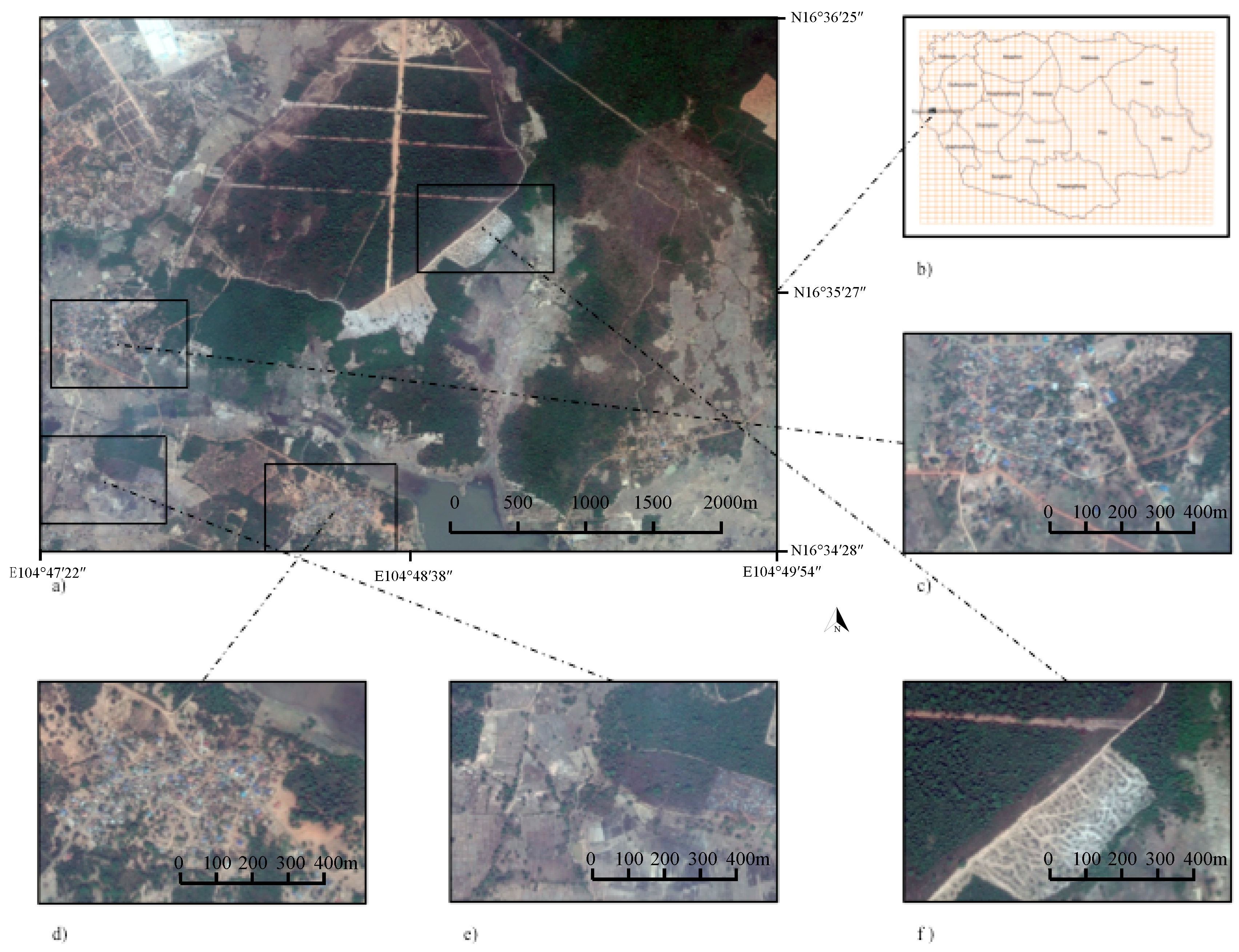
The performances of AdaBoost and CNN are evaluated in Section 4.1 and Section 4.2, respectively. All input training data are contained in the 900 × 600 pixel RGB image shown in Figure 1d. The same image is used for the test data. The test results of the two algorithms are compared and discussed in Section 4.3. In Section 4.4, we test the entire image (Figure 1a, with a size of 3600 × 4500 pixels) by CNN. To enhance the performance, we also alter the input training data. The accuracy of the experiment is evaluated by comparing the result with the ground truth, which contains the tree labels (building areas, non-building areas, and unknown areas such as cloud cover).

4.1. Result of AdaBoost

In the training section, the positive samples contain information of the recognized target, which herein refers to building information; conversely, negative samples are without information of a recognized target such as trees, roads, and unknown areas.

$$H\left(x\right)=sign\left({\displaystyle \sum _{t=1}^T{\alpha }_t{h}_t(x)-Terra}\right)$$

(17)

The confidence obtained by AdaBoost is thresholded by a parameter called Terra. However, when Terra was set to 0 (as in traditional AdaBoost methods), the performance was greatly degraded by the large number of false positives in the classification results. After observing the results for different values of Terra, we selected the optimal Terra based on the Kappa criterion. The following result indicates the progress from using color features to add Haar-like features.

4.1.1. Color Feature

As previously mentioned, the classifier was optimized by trialing four kinds of input samples from Figure 1d. All the testing samples were also prepared from Figure 1d. There must be a one-to-one size correspondence between the testing and training samples, as shown in

Table 3. Training data of color features.

Classifier	Sample Size	Training Samples		Weak Classifiers
		Positive Samples	Negative Samples
AdaBoost_A	1 × 1	48,951	124,803	500
AdaBoost_B	3 × 3	40,071	102,163	500
AdaBoost_C	5 × 5	32,079	81,787	500
AdaBoost_D	7 × 7	24,975	63,675	500

. Since the edges are ignored, the number of testing samples differs among the tests.

After the training procedure, four kinds of stronger classifier emerged: AdaBoost_A–D.

To test the accuracy of classifiers generated in the training part, we utilize the classifiers obtained to detect the testing samples, respectively, and the results are as follows (

Table 4. Comparison of accuracy based on color features.

Classifier	Testing Samples	Terra	Kappa	Overall Accuracy
AdaBoost_A	540,000	1.7	0.306	95.64%
AdaBoost_B	537,004	3.5	0.306	96.04%
AdaBoost_C	534,016	5.0	0.294	96.16%
AdaBoost_D	534,016	8.5	0.283	96.65%

).

As we can infer from the result table, classifier B has the optimum solution, with a Kappa of 0.306 and overall accuracy of 96.04%.

4.1.2. Haar-Like Features + Color Features

To enhance the accuracy of the classifier, we incorporate Haar-like features and color features to mine deeper texture information of the target. Based on the feature value theory, by calculating the entire feature value via an integral image algorithm, the AdaBoost method can be achieved.

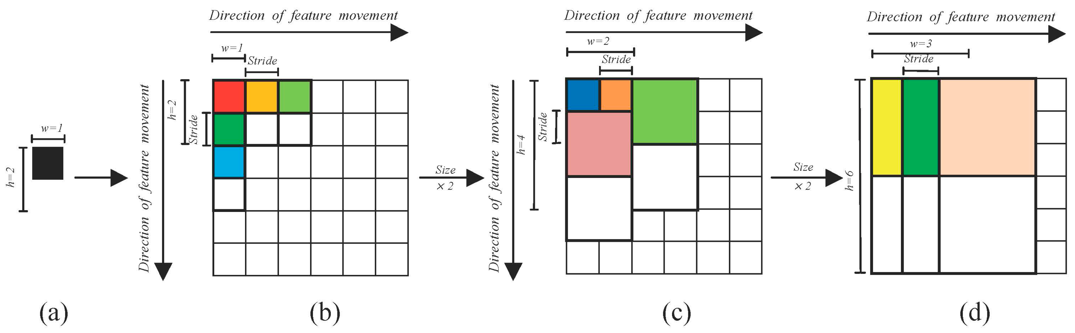
The training samples are captured from Figure 1d, with 111 pieces of positive sample and 283 negative samples, all sized at 25 × 25 pixels in gray-scale. The positive and negative samples are the gray-scale images of buildings and non-buildings, respectively. The input training data is a matrix of Haar-like feature values. The size of the Haar-like features can be stretched or reduced, and they can move within the entire image. The dimension of a two-rectangle feature would reach 3328; therefore, considering that the dimension of the input training data is extremely large, only four kinds of common Haar-like feature have been used. Based on the principle of Figure 2, the total dimension of the input features is 3328 × 2 + 2600 + 2276 = 11532. The testing data is also shown in Figure 1d. After combining with the color features, the result of the identification is enhanced to Kappa of 0.312 and the overall accuracy is enhanced to 96.22%. Compared with the result of using color features only, this result is somewhat improved.

4.2. Result of CNN

In the CNN algorithm training process, placing the training samples and their relevant labels together is necessary. To test the influence of the input parameters on the final classifier, we utilize a control variate method as follows (

Table 5. Training data of CNN.

Classifier	Sample Size	Positive Samples	Negative Samples	Iteration
CNN_A	18 × 18	13,300	50,000	50
CNN_B	18 × 18	13,300	50,000	300
CNN_C	18 × 18	26,150	50,000	300

).

After the training part of CNN, three different classifiers are generated from CNN_A to CNN_C. After utilizing the classifiers to test the given figure, the result and the corresponding figure will be produced (

Table 6. Comparison of accuracy based on CNN.

Classifier	Kappa	Overall Accuracy
CNN_A	0.408	93.96%
CNN_B	0.433	94.13%
CNN_C	0.564	96.30%

).

Compared with the respective results, the obtained classifier CNN_C performs well in detecting the buildings from the given figure. Kappa is enhanced to 0.564 and the overall accuracy reaches 96.30%. In such cases, the confusion matrix and the outcome figures are as follows (

Table 7. Confusion matrix based on CNN in pixel.

True Positives: 12,540	False Positives: 17,366
False Negatives: 799	True Negatives: 459,034

).

As we mentioned in the definition of the confusion matrix, in the method based on CNN, actual buildings that were correctly classified as buildings is 12,540, non-buildings incorrectly labeled as buildings is 17,366, buildings that were incorrectly marked as non-buildings is 799, and number of correctly classified non-buildings is 459,034. Although the number of non-buildings that were incorrectly labeled as buildings is a little bit high, impacting the performance of the result, other parts of the matrix perform well.

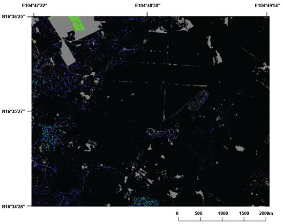
In the outcome figure of CNN_C, gray refers to the unknown part, green means the actual buildings that were correctly classified as buildings, blue indicates the non-buildings that were incorrectly labeled as buildings, red shows the buildings that were incorrectly marked as non-buildings, and black denotes the correctly classified non-buildings. As shown in the result, the CNN_C classifier has high performance in detecting buildings. In Figure 4b, it can be seen that the classification error decreases stably as the iteration increases.

4.3. Comparison and Discussion

We utilized machine learning methods including AdaBoost and CNN to identify buildings from remote sensing images and generated the relative testing results, as mentioned in Section 4.1 and Section 4.2, respectively. Inferring from the comparisons in accuracy, the best result of Kappa and overall accuracy are 0.312% and 96.20% in the AdaBoost algorithm, respectively, whereas in CNN, the result is enhanced to 0.564% and 96.30%, respectively. According to the comparison, in the corresponding testing area, the Kappa of our CNN method is approximately 25% higher than that of AdaBoost. For overall accuracy, CNN also outperforms AdaBoost.

Note that the traditional visual interpretation of remote sensing images is a complex and time-consuming process. Although it has very high accuracy, it is not suited to large-scale automation projects. The effect of AdaBoost methods is highly dependent on the training feature. The color and Haar-like features chosen in our experiment cannot express all the helpful and useful features of the buildings, which impacts the accuracy of the result. In contrast, CNN can mine and extract deeper information on the input features of building, which can be helpful in identification.

4.4. Practical Application

In this section, we demonstrate how the CNN method works via the entire image in Figure 1a, which is 30 times bigger than that in Figure 1d. We compare two kinds of input training data and separately obtain the identification results as follows (

Table 8. Different training data using CNN.

Training Type	Input Training Area	Positive Samples	Negative Samples
Train_A	Figure 1c,d	26,150	50,000
Train_B	Figure 1c–f	26,150	150,000

).

The training data in type Train_B contains more diverse negative sample information than that in Train_A, with 150,000 samples including information of mountains and other types of land. The identification results are as follows (

Table 9. Comparison of accuracy based on CNN.

Training Type	TP	FP	FN	TN	Kappa	Overall Accuracy
Train_A	82,578	265,923	12,306	15,009,525	0.366	98.19%
Train_B	83,351	175,495	11,533	15,099,953	0.466	98.78%

).

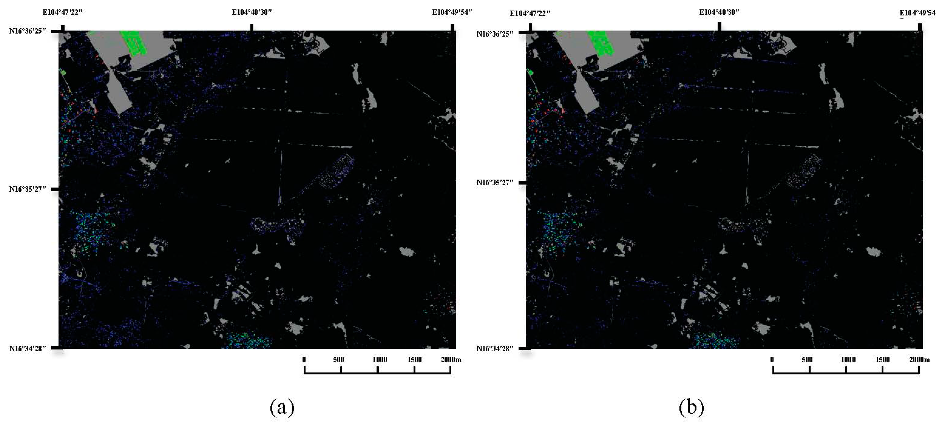
As observed from the testing result, the Kappa and overall accuracy increase when the negative training samples are expanded. In Figure 4, most of the village buildings can be identified, but the inaccuracy points are mainly distributed in the village boundary and some building-like areas. From Figure 5b, areas such as mountains can be identified as non-buildings areas, whereas they could not be detected in Figure 5a.

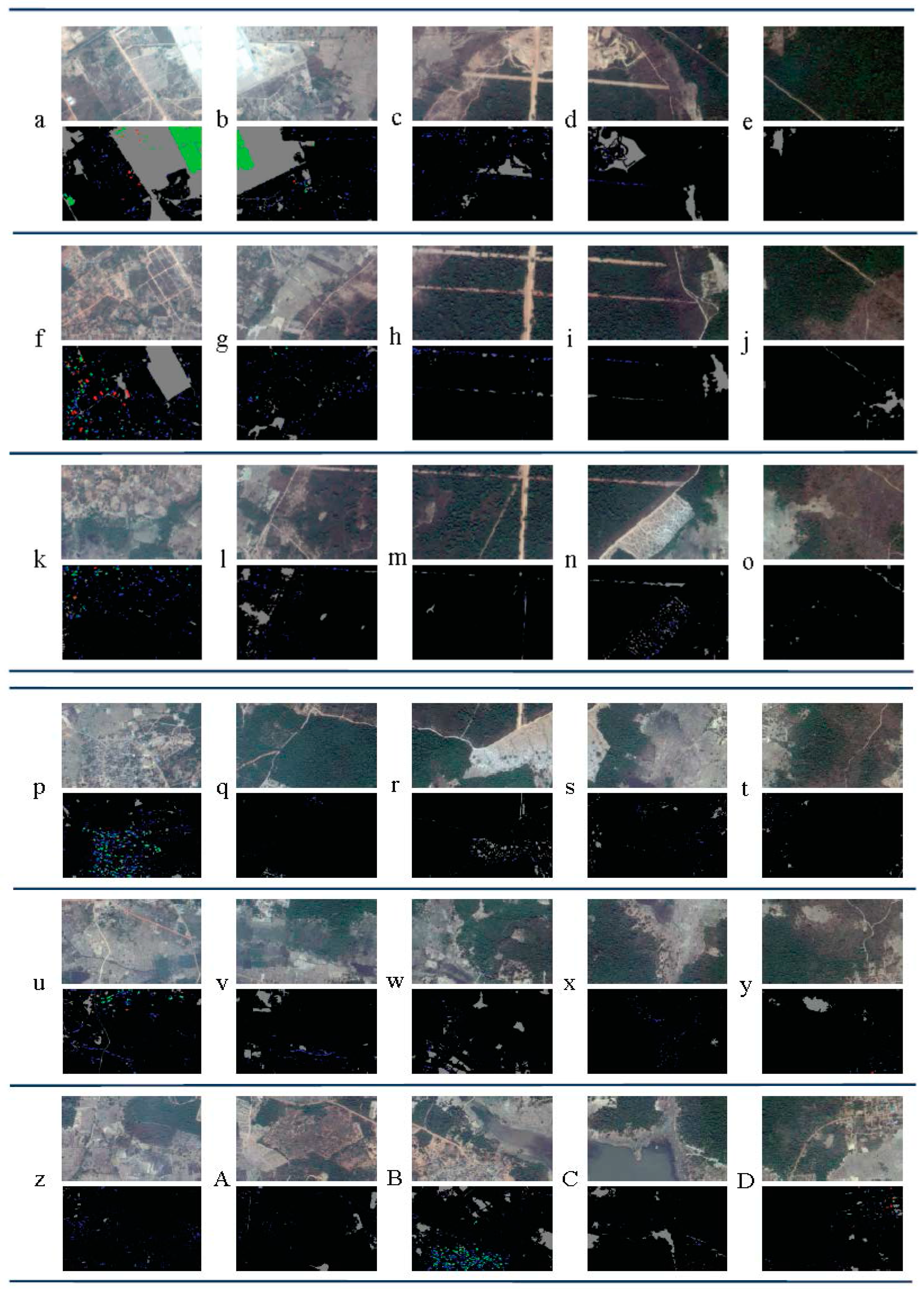
To detect the details of the performance of Train_B, we split the image into 30 small images of size 900 × 600 pixels as follows (Figure 6).

The performance of each part is different and the accuracy comparison is as follows.

For different study areas, the overall accuracy of the CNN method can be up to 99.00%. We only show part of the results in

Table 10. Accuracy assessment of all the testing data in Figure 4 based on CNN.

Study Area	Number of Positive Pixels	Number of Negative Pixels	Kappa	Overall Accuracy
a	41,262	307,805	0.888	97.54%
b	14,392	398,102	0.761	98.00%
B	9075	495,639	0.470	96.47%

, especially those containing information of buildings (positive pixels) where Kappa can be up to 0.888, which indicates high performance. We can also infer that the overall accuracy of the proposed method is considerably stable in different areas. As Kappa is relatively low in some areas, identification accuracy can be improved by expanding the training data, as shown in previous processes.

In general, the experimental results indicate that our proposed method based on machine learning, especially on CNN, has high performance in remote sensing identification of buildings.

5. Conclusions and Future Work

In this paper, we propose two kinds of supervised machine learning methods for building identification based on GE images. The corresponding machine learning methods AdaBoost and CNN help us obtain building identification classifiers by training the designed samples. Applying the obtained AdaBoost and CNN classifiers to automatically extract information of buildings from the remote sensing images generates the identification maps of buildings.

The proposed method shows the ability of supervised machine learning in village mapping, which is experimentally demonstrated by including several kinds of areas in Kaysone. The obtained classifier can be used for all cases and no manual interaction is needed. Our method of CNN achieves a Kappa of 0.564 and an overall accuracy of 96.30%, which is comparable to those of AdaBoost and other methods.

Furthermore, the proposed method can be efficiently utilized in remote sensing recognition of not merely buildings. By training the prior knowledge of the corresponding identification samples, the proposed method can generate a classifier that has the ability to classify relative targets and leads to promising classification results. Therefore, based on the result of this experiment, our proposed method is a promising approach that might be applied to many potential applications in the near future.

Although this study indicates that the proposed method could be efficiently used in building identification, further and more detailed exploration on the method is required in the future. First, to test the method’s stability, more extended and sophisticated areas need to be tested. Second, to alleviate the labor-intensive task of training the data, we will apply the learned model of one area to other areas with similar landscapes. Unfortunately, the spectral characteristics of remote sensing images respond to the varying conditions of image capture. To improve the performance in such cases, we will consider a transfer learning technique. Third, we will apply the proposed method to other feature identifications in high-resolution remote sensing images, such as roads and agricultural land. We are also interested in extending this method to classifications of multi-class landscapes. We believe that the proposed method has great practical value for solving diverse classification problems.

References

1. Younan, N.H.; Aksoy, S.; King, R.L. Foreword to the special issue on pattern recognition in remote sensing. IEEE J. Sel. Topics Appl. Earth Obs. Remote Sens. 2012, 5, 1331–1334. [Google Scholar] [CrossRef] [Green Version]
2. Xu, X.; Xing, H. M8.0 Wenchuan Earthquake; Springer: Heidelberg, Germany; London, UK, 2011. [Google Scholar]
3. Davics, J.J.; Beresford, A.R.; Hopper, A. Scalable, distributed, real-time map generation. IEEE Pervasive Comput. 2006, 5, 47–54. [Google Scholar]
4. Fan, J.; Chen, J.X.; Tian, B.; Yan, D.; Cheng, G.; Cui, P.; Zhang, W. Rapid assessment of secondary disasters induced by the Wenchuan earthquake. Comput. Sci. Eng. 2010, 12, 10–19. [Google Scholar] [CrossRef]
5. Gallent, N. Introduction to Rural Planning; Routledge: London, UK; New York, NY, USA, 2008. [Google Scholar]
6. Kiefer, R.W.; Lillesand, T.M.; Chipman, J.W. Remote Sensing and Image Interpretation; John Wiley & Sons: Hoboken, NJ, USA, 2008. [Google Scholar]
7. Richards, J.A.; Jia, X. Remote sensing Digital Image Analysis: An Introduction; Springer: Berlin, Germany, 2006. [Google Scholar]
8. Schowengerdt, R.A. Remote Sensing: Models and Methods for Image Processing; Elsevier Academic Press: Amsterdam, The Netherlands; Tokyo, Japan, 2007. [Google Scholar]
9. Bégué, A.; Vintrou, E.; Ruelland, D.; Claden, M.; Dessay, N. Can a 25-year trend in Soudano-Sahelian vegetation dynamics be interpreted in terms of land use change? A remote sensing approach. Glob. Environ. Chang. 2011, 21, 413–420. [Google Scholar] [CrossRef]
10. Wu, W.; Shibasaki, R.; Yang, P.; Zhou, Q.; Tang, H. Remotely sensed estimation of cropland in China: A comparison of the maps derived from four global land cover datasets. Can. J. Remote Sens. 2008, 34, 467–479. [Google Scholar] [CrossRef]
11. Yu, X.; Zhang, A.; Hou, X.; Li, M.; Xia, Y. Multi-temporal remote sensing of land cover change and urban sprawl in the coastal city of Yantai, China. Int. J. Digit. Earth 2012, 6, 1–18. [Google Scholar] [CrossRef]
12. Zhou, H.; Aizen, E.; Aizen, V. Deriving long term snow cover extent dataset from AVHRR and MODIS data: Central Asia case study. Remote Sens. Environ. 2013, 136, 146–162. [Google Scholar] [CrossRef]
13. Long, J.B.; Giri, C. Mapping the Philippines’ mangrove forests using Landsat imagery. Sensors 2011, 11, 2972–2981. [Google Scholar] [CrossRef] [PubMed]
14. Laliberte, A.S.; Browning, D.M.; Rango, A. A comparison of three feature selection methods for object-based classification of sub-decimeter resolution Ultracam-L imagery. Int. J. Appl. Earth Obs. 2012, 15, 70–78. [Google Scholar] [CrossRef]
15. Duro, D.C.; Franklin, S.E.; Dubé, M.G. A comparison of pixel-based and object-based image analysis with selected machine learning algorithms for the classification of agricultural landscapes using SPOT-5 HRG imagery. Remote Sens. Environ. 2012, 118, 259–272. [Google Scholar] [CrossRef]
16. Guo, J.; Liang, L.; Gong, P. Removing shadows from Google Earth images. Int. J. Remote Sens. 2010, 31, 1379–1389. [Google Scholar] [CrossRef]
17. Potere, D. Horizontal positional accuracy of Google Earth’s high-resolution imagery archive. Sensors 2008, 8, 7973–7981. [Google Scholar] [CrossRef]
18. Hu, Q.; Wu, W.; Xia, T.; Yu, Q.; Yang, P.; Li, Z.; Song, Q. Exploring the use of Google Earth imagery and object-based methods in land use/cover mapping. Remote Sens. 2013, 5, 6026–6042. [Google Scholar] [CrossRef]
19. Yu, L.; Gong, P. Google Earth as a virtual globe tool for earth science applications at the global scale: Progress and perspectives. Int. J. Remote Sens. 2011, 33, 3966–3986. [Google Scholar] [CrossRef]
20. Drǎguţ, L.; Tiede, D.; Levick, S.R. ESP: A tool to estimate scale parameter for multiresolution image segmentation of remotely sensed data. Int. J. Geogr. Inf. Sci. 2010, 24, 859–871. [Google Scholar] [CrossRef]
21. Yu, Q.; Gong, P.; Clinton, N.; Biging, G.; Kelly, M.; Schirokauer, D. Object-based detailed vegetation classification with airborne high spatial resolution remote sensing imagery. Photogramm. Eng. Remote Sens. 2006, 7, 799–811. [Google Scholar] [CrossRef]
22. Pal, A.; Pal, S.K. Pattern Recognition: From Classical to Modern Approaches; World Scientific: Singapore, 2001. [Google Scholar]
23. Viola, P.; Jones, M. Rapid object detection using a boosted cascade of simple features. In Proceedings of the 2001 IEEE Computer Society Conference on Computer Vision and Pattern Recognition (CVPR 2001), Kauai, HI, USA, 8–14 December 2011.
24. Zheng, J.; Cui, Z.; Liu, A.; Jia, Y. A k-means remote sensing image classification method based on Adaboost. In Proceedings of the Fourth International Conference on Natural Computation (ICNC ‘08), Jinan, China, 18–20 October 2008; pp. 27–32.
25. Zongur, U.; Halici, U.; Aytekin, O.; Ulusoy, I. Airport runway detection in satellite images by Adaboost learning. Proc. SPIE 2009, 7477. [Google Scholar] [CrossRef]
26. Li, R.; Sun, J.; Wang, J.; Zhu, L.; Liu, R. The study on dynamic extraction of urban land use cover with remote sensing image based on Adaboost algorithm. Proc. SPIE 2009, 7498. [Google Scholar] [CrossRef]
27. Cetin, M.; Halici, U.; Aytekin, O. Building detection in satellite images by textural features and Adaboost. In Proceedings of the 2010 IAPR Workshop on Pattern Recognition in Remote Sensing (PRRS), Istanbul, Turkey, 22 August 2010; pp. 1–4.
28. Bouvrie, J. Notes on Convolutional Neural Networks. Available online: https://www.google.com/url?sa=t&rct=j&q=&esrc=s&source=web&cd=1&ved=0ahUKEwjNuZXSzsnLAhWHspQKHcY-CBwQFgghMAA&url=http%3A%2F%2Fcogprints.org%2F5869%2F1%2Fcnn_tutorial.pdf&usg=AFQjCNGqmw7vLOJXSwyHyS6SPTDD5VOiGg&bvm=bv.117218890,d.dGo&cad=rja (accessed on 10 November 2015).
29. Chen, X.; Xiang, S.; Liu, C.-L.; Pan, C.-H. Vehicle detection in satellite images by parallel deep convolutional neural networks. In Proceedings of the 2013 2nd IAPR Asian Conference on Pattern Recognition (ACPR), Naha, Japan, 5–8 November 2013; pp. 181–185.
30. Li, B.-Q.; Li, B. Building pattern classifiers using convolutional neural networks. In Proceedings of the International Joint Conference on Neural Networks (IJCNN ‘99), Washington, DC, USA, 10–16 July 1999; pp. 3081–3085.
31. Yue, J.; Zhao, W.Z.; Mao, S.J.; Liu, H. Spectral-spatial classification of hyperspectral images using deep convolutional neural networks. Remote Sens. Lett. 2015, 6, 468–477. [Google Scholar] [CrossRef]
32. Lee, S.; Zhang, H.; Crandall, D.J. Predicting geo-informative attributes in large-scale image collections using convolutional neural networks. IEEE Comput. Soc. 2015, 550–557. [Google Scholar]
33. Sermanet, P.; Chintala, S.; LeCun, Y. Convolutional neural networks applied to house numbers digit classification. In Proceedings of the 2012 21st International Conference on Pattern Recognition, Tsukuba, Japan, 11–15 November 2012; pp. 3288–3291.
34. Hu, F.; Xia, G.; Hu, J.; Zhang, L. Transferring deep convolutional neural networks for the scene classification of high-resolution remote sensing imagery. Remote Sens. 2015, 7, 14680–14707. [Google Scholar] [CrossRef]
35. Mammone, A.; Turchi, M.; Cristianini, N. Support vector machines. Comput. Stat. 2009, 1, 283–289. [Google Scholar] [CrossRef]
36. Dou, J.; Chang, K.T.; Chen, S.S.; Yunus, A.P.; Liu, J.K.; Xia, H.; Zhu, Z.F. Automatic case-based reasoning approach for landslide detection: Integration of object-oriented image analysis and a genetic algorithm. Remote Sens. 2015, 7, 4318–4342. [Google Scholar] [CrossRef]
37. Li, X.J.; Cheng, X.W.; Chen, W.T.; Chen, G.; Liu, S.W. Identification of forested landslides using Lidar data, object-based image analysis, and machine learning algorithms. Remote Sens. 2015, 7, 9705–9726. [Google Scholar] [CrossRef]
38. Attarchi, S.; Gloaguen, R. Classifying complex mountainous forests with l-band SAR and Landsat data integration: A comparison among different machine learning methods in the hyrcanian forest. Remote Sens. 2014, 6, 3624–3647. [Google Scholar] [CrossRef]
39. Jing, W.; Yang, Y.; Yue, X.; Zhao, X. Mapping urban areas with integration of DMSP/OLS nighttime light and MODIS data using machine learning techniques. Remote Sens. 2015, 7, 12419–12439. [Google Scholar] [CrossRef]
40. Bishop, C.M. Pattern Recognition and Machine Learning; Springer: New York, NY, USA, 2006. [Google Scholar]
41. Mozos, O.M.; Stachniss, C.; Burgard, W. Supervised learning of places from range data using AdaBoost. In Proceedings of the 2005 IEEE International Conference on Robotics and Automation (ICRA 2005), Barcelona, Spain, 18–22 April 2005; pp. 1730–1735.
42. Yoav, F.; Schapire, R. A decision-theoretic generalization of on-line learning and an application to boosting. J. Comput. Syst. Sci. 1997, 55, 119–139. [Google Scholar]
43. Ng, A.; Ngiam, J.; Foo, C.Y.; Mai, Y.; Suen, C. Unsupervised Feature Learning and Deep Learning (UFLDL). Available online: http://ufldl.stanford.edu/wiki/index.php/UFLDL_Tutorial (accessed on 2 November 2015).
44. Palm, R.B. Prediction as a Candidate for Learning Deep Hierarchical Models of Data. Master’s Thesis, Technical University of Denmark, DTU Informatics, Lyngby, Denmark, 2012. [Google Scholar]
45. Carletta, J. Assessing agreement on classification tasks: The kappa statistic. Comput. Linguist. 1996, 22, 249–254. [Google Scholar]
Figure 1. Kaysone area (a); located in Savannakhet Province, Laos (b). Panels (c) and (d) are enlarged views of typical village areas; and (e) and (f) show mountain and vegetation areas with similar tones to buildings. The resolution of all images (except (b)) is 1 m.
Remotesensing 08 00271 g001
Figure 2. Haar-like feature’s size change and movement: (a) Original 2 × 1 feature; (b) movement of original feature; (c) 4 × 2 feature; and (d) 6 × 3 feature.
Remotesensing 08 00271 g002
Figure 3. Convolution and pooling process.
Remotesensing 08 00271 g003
Figure 4. (a) Classification result of CNN_C; and (b) classification error.
Remotesensing 08 00271 g004
Figure 5. Classification results of CNN: (a) Train_A; and (b) Train_B.
Remotesensing 08 00271 g005
Figure 6. Classification results (a-D) of test areas using CNN_C.
Remotesensing 08 00271 g006