Use of High-Quality and Common Commercial Mirrors for Scanning Close-Range Surfaces Using 3D Laser Scanners: A Laboratory Experiment


1
Department of Civil Engineering, University of Alicante, 03690 San Vicente del Raspeig, Alicante, Spain
2
Department of Optics, Pharmacology and Anatomy, University of Alicante, 03690 San Vicente del Raspeig, Alicante, Spain
*
Author to whom correspondence should be addressed.
Remote Sens. 2017, 9(11), 1152; https://doi.org/10.3390/rs9111152
Submission received: 22 September 2017
/
Revised: 3 November 2017
/
Accepted: 7 November 2017
/
Published: 10 November 2017
(This article belongs to the Special Issue Uncertainty in Remote Sensing Image Analysis)
Abstract
:Three Dimension (3D) laser scanners enable the acquisition of millions of points of a visible object. Terrestrial laser scanners (TLS) are ground-based scanners, and nowadays the available instruments have the ability of rotating their sensor in two axes, capturing almost any point. Since many sensors can only operate in a vertical position, they cannot capture points located beneath themselves. Consequently, these instruments are generally unable to capture data in a vertical descending direction. Moreover, since the device positioning has certain requirements of space and terrain stability, it is possible that specific regions of interest are outside the reach of the laser. A possible solution is to address the laser beam towards the desired direction by means of a mirror. Common mirrors are very cheap; therefore, they are easy to manipulate and to substitute in case they get broken. However, due to their careless fabrication process, it seems reasonable to think that they are unprecise. In contrast, front-end mirrors are more expensive and delicate, and consequently, deflecting angles are more precise. In this research, we designed a laboratory test to analyze the arising noise when standard and high-quality mirrors are used during the TLS scanning process. The results show that the noise introduced when scanning through a standard mirror is higher than that produced when using a high-quality mirror. However, both cases show that this introduced error is lower than the instrumental error. As a result, this study concludes that it is reasonable to use standard mirrors when scanning in similar conditions to this laboratory test.

1. Introduction
Remote sensing techniques enable the acquisition of 3D information of objects or surfaces with high accuracy and high spatial resolution [1]. 3D laser scanners (3DLS) are light detection and ranging (LiDAR)-based instruments that consist basically of a transmitter/receiver of a laser beam and a scanning device [2]. These instruments employ a laser that produces or emits a light beam. They are used to determine ranges in two methods: phase (phase-based) and pulse (time-of-flight). Phase-based devices generally allow better accuracy but lower range, while time-of-flight devices allow greater range [3]. Both sensors send laser pulses to objects. The signal returns to the sensor and it is recorded. Some instruments orient the laser through a set of mirrors that enable it to know the orientation of the laser in a local reference system. Time-of-flight instruments measure the time (Δt) employed by the signal to return, and as the speed of signal is known (the speed of light c), the distance (d) can be calculated (1). Phase-based instruments measure the number of phases (N), which along with the wavelength (λ) allow the calculation of the distance [4]. As the orientation is known, the coordinates relative to the scanning point of the reflective surface can be calculated (2).
3DLS devices have been widely analyzed and researchers have tested the quality of measurements [5], the luminance of the laser radiation for the classification of materials [6], the effect of the angle of incidence to the target surface [7,8,9] or the color of the scanned surface [9]. 3DLS devices are classified according to the position of the sensor, such as aerial laser scanners (ALS) referred to as airborne-based scanners [10,11]; mobile laser scanners that are installed on vehicles (MLS) [12]; personal laser scanners that are carried in a backpack [13,14]; offshore laser scanners used for boats (OLS) [15,16], and terrestrial laser scanners (TLS), which are ground-based scanners [3,17]. Nowadays these techniques are widely used for a number of applications, such as agriculture [18], archaeology [19], autonomous vehicles [20], robotics [21], geology [22], mining [23], rock mechanics [3], etc.
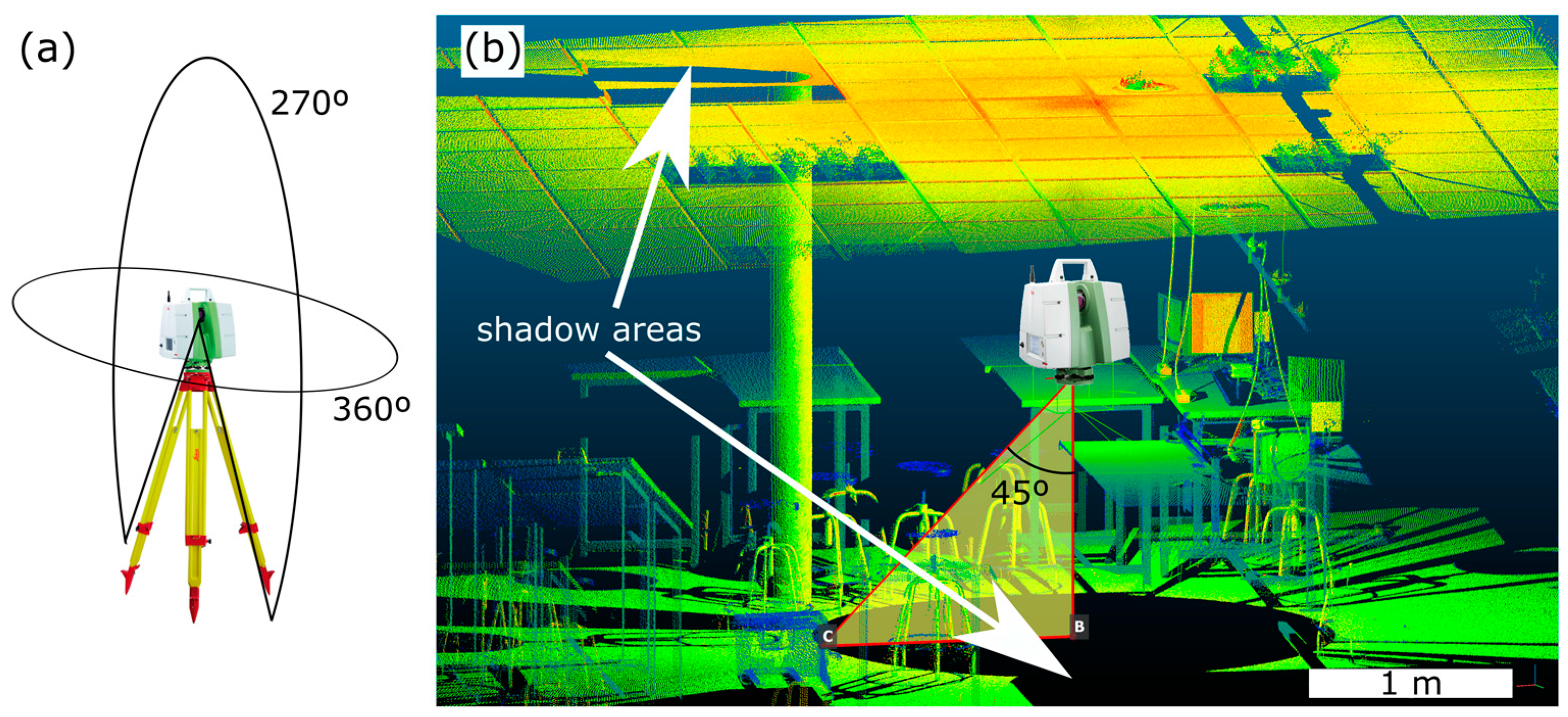
When using ground-based instruments, the laser can only register points that are along its line-of-sight. The areas behind visible objects are shadow areas (occlusions) [24]. This issue is usually solved combining different scanning stations or even combining different techniques [3]. Some models of 3D laser scanners are fixed devices, so they can only scan a portion of the space while other can rotate around a vertical axis, so its maximum horizontal field of view is 360°. However, as TLS are usually fixed on a tripod, their maximum vertical field-of-view is limited by the system’s physical support. For instance, Figure 1a shows a 3D laser scanner model Leica C10 with a maximum vertical field-of-view of 270° when the sensor is horizontally leveled. This means that there is a shadow area beneath the device due to its framework and the supporting system. This problem could be solved by changing the orientation of the device; that is, anchoring the device in a wall (for example) in order to have a90° shadow on the wall. Unfortunately, the TLS manufacturer recommends that the base of the sensor only be horizontal in order for good functioning. Figure 1b shows the scanning of a laboratory. It can be observed that there is a circular shadowed area under the device, and others behind the piles or other objects.
The shadowing problem is not limited to the region under the scanner. Notice that in some applications there is no possibility to trace a straight line between the sensor and the region of interest. This is the case when one is scanning into a vertical tube, such as the bottom of open-ended piles or when there are occluded areas that shadow part of the space [24]. In all these cases, a possible solution is to use external mirrors to address the beam in the desired direction.
The use or presence of mirrors in the scanning process has been already analyzed in the literature. Actually, it is a popular topic in simultaneous localization and mapping (SLAM) [25]. Efforts have been made to automate the detection of mirror frames and to correct mirror reflection when using a laser sensor in robotics [25]. Additionally, mirrors have also been used for enhancing the 3D scanning of objects (i.e., cultural heritage) [26]. Some works have used small front-surface mirrors (250 × 100 mm and 400 × 400 mm) [26], which are more accurate than common commercial mirrors but they are delicate to handle, have limited sizes and are not very cost-effective. However, to the best of our knowledge, the accuracy obtained using common mirrors has not been analyzed until now, despite their availability and low cost.
The objective of this work is to determine whether common and front-end mirrors can be employed to address the laser beam and how their use affects to the dataset with respect to a direct scan. To answer this question, we analyze the accuracy of a close-range (~300 m) TLS when the beam is deflected by a planar mirror. We also analyze the influence of the mirror surface quality in the results. To this end we designed an experiment in which a planar surface was scanned using a TLS model Leica ScanStation C10 at 10 m. The direct measurements were compared with those obtained after having the beam reflected in two different planar mirrors: one common mirror and one front-end mirror.
2. Materials and Methods
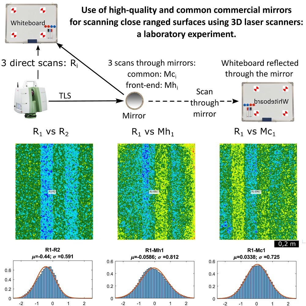
To evaluate how the scanning process through a mirror affects the accuracy, a laboratory experiment was designed. Basically, the test consisted of the scanning of a whiteboard in three ways: (1) direct scanning, (2) through a high-quality front-surface mirror and (3) through a common commercial mirror. The comparison of the measurements done directly with those obtained through the mirror provides the error obtained when the measurement is taken through an intermediate reflection.
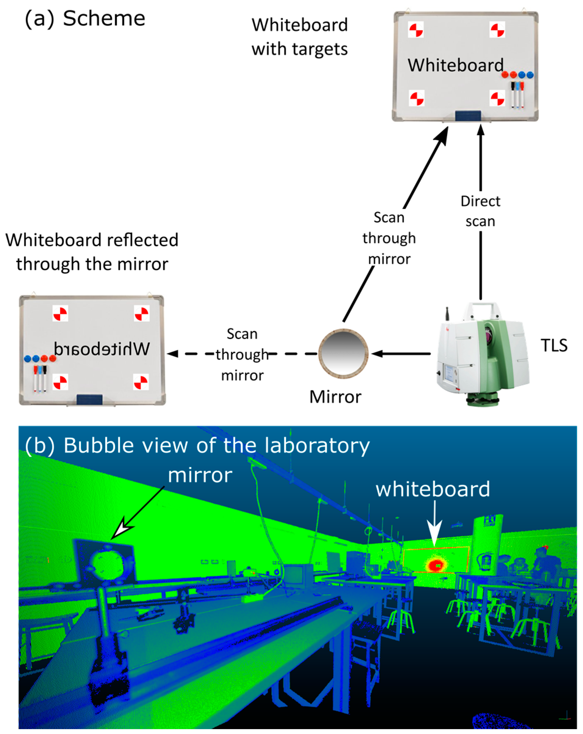
The test was conducted in a laboratory under controlled illumination conditions. Figure 2a shows a scheme of the laboratory with the location of the TLS, the mirror and the whiteboard. A 3D laser scanner model Leica C10 was used. Its angular accuracy is 12′′, the distance accuracy is 4 mm and the noise is 2 mm at 50 m [27].
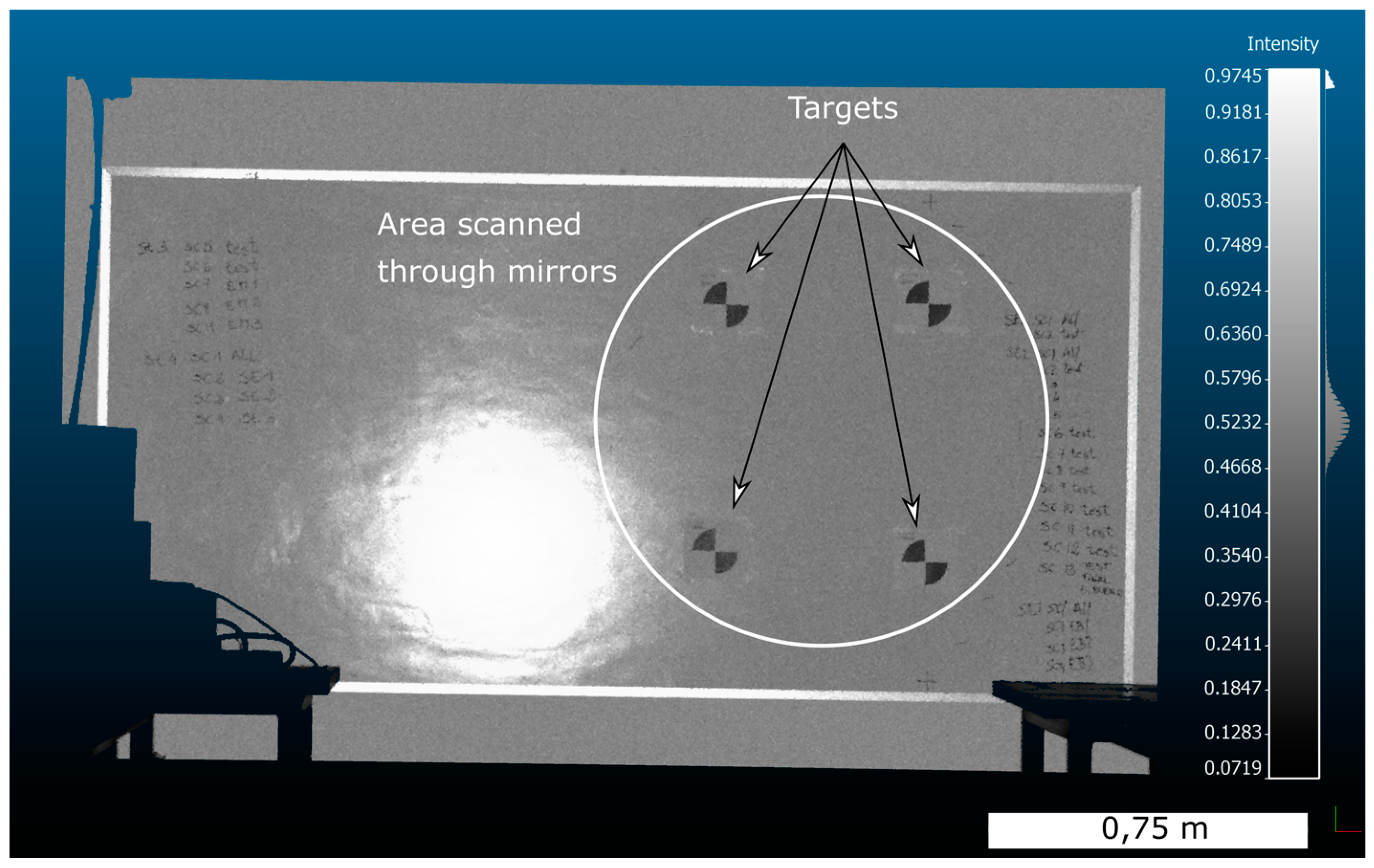
The scan station was located at 7.5 m from the whiteboard. The distance from the station and the mirror was 1 m (Figure 2b). The mirrors were mounted on an adjustable plate so they could be accurately oriented. Finally, the direct scanning ray reached the test surface almost in the normal direction. For the indirect configuration, the angle between the laser beam and the normal to the mirror surface was 45°, while the reflected beam arrived to the surface test at an incidence angle of around 8°. In order to enable a success scanning process, all existing objects between all elements involved (the whiteboard, the TLS and the mirror) were removed. The scanned surface was a portion of a common whiteboard placed on a wall. Four black and white HDS targets were distributed, delimiting the area of interest (Figure 3). The scan was conducted both directly and through two different mirrors. The first mirror was a planar front-surface silica mirror of 50.8 mm of diameter and 15.9 mm of thickness, with a surface accuracy of λ/20 for a λ (wavelength) of 633 nm. This means that the maximum deviation from a planar surface that can be found in this mirror is 31.65 nm. The second mirror was a standard old planar second front mirror with some scratches in the surface.
The methodology is shown in the chart depicted in Figure 4 and is described as follows. Stage one consists of the scanning of the whiteboard. Firstly, the area of interest was scanned in a single scan station and three different steps. The scanning resolution was set to the highest (i.e., separation between points of 2.5 cm at 100 m). In the first step of scanning, the whiteboard was scanned three times directly, without the use of any mirror. As a result, three point clouds were obtained: R1, R2 and R3. In the second step, a high-quality mirror was installed at 1 m from the TLS and it was oriented so that the laser beam reached the points of the area of interest. The area of interest was scanned three times, obtaining the point clouds Mh1, Mh2 and Mh3. In the last step, the previous mirror was substituted by a common mirror, oriented as before. Then, the area of interest was again scanned three times obtaining the point clouds Mc1, Mc2 and Mc3. During the full process, the TLS was not moved from its original location.
Stage two consists of a basic transformation of the 3D point clouds acquired through the mirrors. Due to the specular reflection, the law of reflection states that the obtained image is symmetrical to the original. Due to this, a transformation is required [28] in order to enable the comparison of the different point clouds. As it is a planar transformation, it is addressed by changing the sign of one coordinates; in our particular case the coordinate changed was x. As the result of this transformation, the point clouds Mh1′, Mh2′, Mh3′, Mc1′, Mc2′ and Mc3′ were obtained.
Stage three consists of the alignment of all the clouds to enable the comparison within the same reference system. Firstly, all the coordinates of the targets of the point clouds R1, Mh1′ and Mc1′ were extracted. Targets consist of four circular sectors (Figure 3) with two different colors. By means of edge detection, the line between sectors was detected. This enabled the calculation of the coordinates of the center of the targets. More details about this procedure can be found in [29]. Then, using those coordinates the transformation of Mh1′ and Mc1′ to R1 was calculated, obtaining the rigid transformation matrices Kh and Kc, respectively, through the least square method. The rigid transformation matrices are defined by a translation vector (Tx, Ty, Tz) and the Euler angles. The transformation Kh was applied to the group of point clouds Mh1′, Mh2′ and Mh3′, obtaining the point clouds Mh1′′, Mh2′′ and Mh3′′. The same procedure was performed with Mc1′, Mc2′ and Mc3′, applying the transformation Kc and obtaining the point clouds Mc1′′, Mc2′′ and Mc3′′. As the transformation matrices were obtained in order to minimize the error for the first measurement (for both mirrors), using these matrices in the rest of measurements will provide information about the errors obtained through different scans from the same station, which is a common practice.
Finally, stage four consists of the comparison of the point clouds scanned directly (R1, R2 and R3) with those scanned through the mirrors (Mh1′′, Mh2′′, Mh3′′, Mc1′′, Mc2′′ and Mc3′′) (Figure 4). First, a rectangular area (0.66 × 0.78 m) was cropped to all the point clouds simultaneously. Prior to further analysis, each point cloud was fitted to a planar surface in order to confirm that all of them were statistically equivalent. These calculations showed that all the clouds fit to the same plane within 95% of confidence bounds, with equivalent mean squared errors. After this preliminary analysis, all the clouds where compared in pairs.
The compared point clouds are shown in Figure 4 (Stage 4) The comparison was performed calculating the normal distance between the point clouds through the method multiscale model to model cloud comparison (M3C2, [30]). The M3C2 method computes the signed distances directly between two point clouds, unlike other methods that compute the nearest neighbor distance (cloud-to-cloud distance) or the normal distance of a meshed surface to a point cloud (cloud-to-mesh distance). In this work, the computed distance is an estimation of the noise and the deformation introduced by the conventional scanning process using different kinds of mirrors. The result of each comparison is a cloud, which is the reference cloud (i.e., R1, R2 or R3), with the estimated error assigned to each point. For each set of points, the mean and standard deviation was calculated.
3. Results
3.1. Comparison of Direct Scans
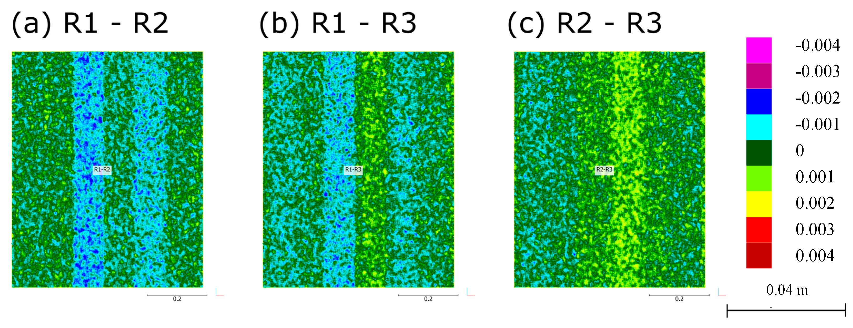
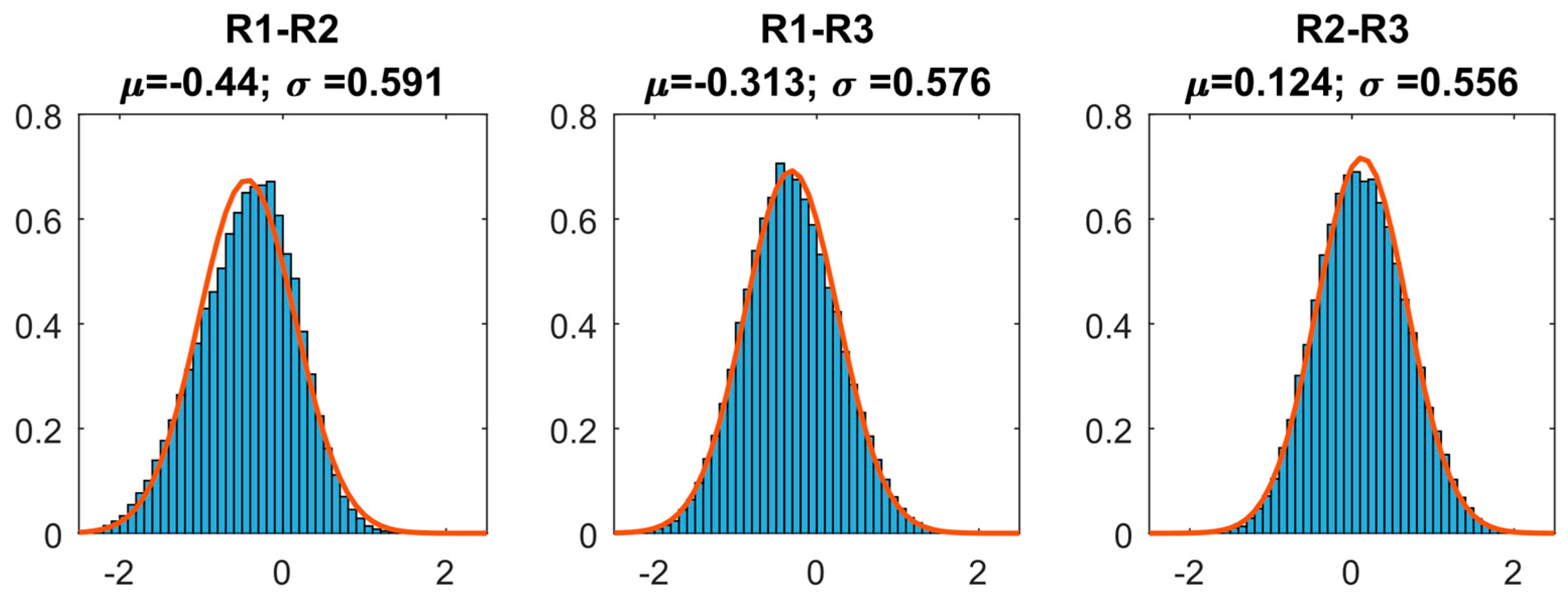
Figure 5 shows the point cloud scanned directly (R1, R2 and R3). For each point, the color shows the M3C2 distance. The observation of Figure 5 indicates that there is a common error pattern in the vertical bands. Figure 6 shows the histograms of those sets with their calculated mean and standard deviation in mm. The absolute mean values of these distributions range from 0.12 to 0.44 mm, which provide an idea of the instrumental error. Additionally, the standard deviation of the error is around 0.58 mm for all the three cases.
3.2. Errors Found When Scanning through a High-Quality Mirror
The transformation matrix Kh for this case is shown in (3). The obtained root mean square (RMS) of the least square method was 0.00111955 m.
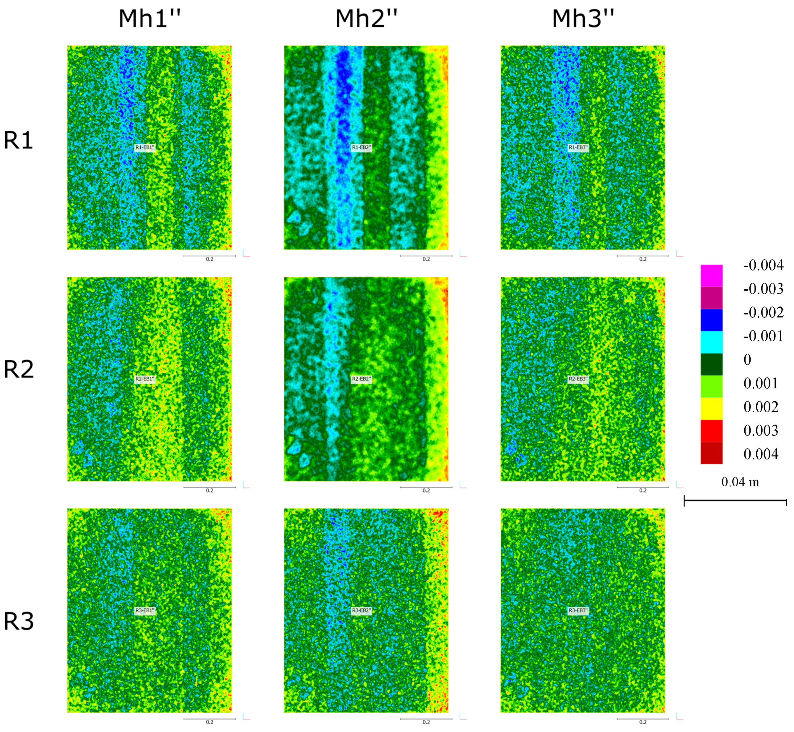
Figure 7 shows the point cloud scanned directly (R1, R2 and R3) compared to the data acquired through the high-quality mirror. For each point, the color shows the M3C2 distance. Figure 8 shows the histograms of those sets with their calculated mean and standard deviation in mm.
The vertical band errors presented in the previous section appear again in the case R1-Mh1′′. This effect is attenuated in the rest of the comparisons. Mean and standard deviations are shown in Figure 8. The absolute minimum mean value is found in the case R1-Mh1′′ (0.06 mm), as was expected, because the Mh1′′ cloud was registered to the R1 cloud using the least square method. The rest of the absolute mean values range from 0.11 to 0.36 mm. The standard deviation remains stable, ranging from 0.62 to 0.81 mm, which is a slightly higher result than in the previous case with the direct scanning. It is noteworthy that the registration matrix applies a rigid transformation, so the clouds are only translated and rotated, and no deformation is applied. Therefore, the standard deviation should not be affected.
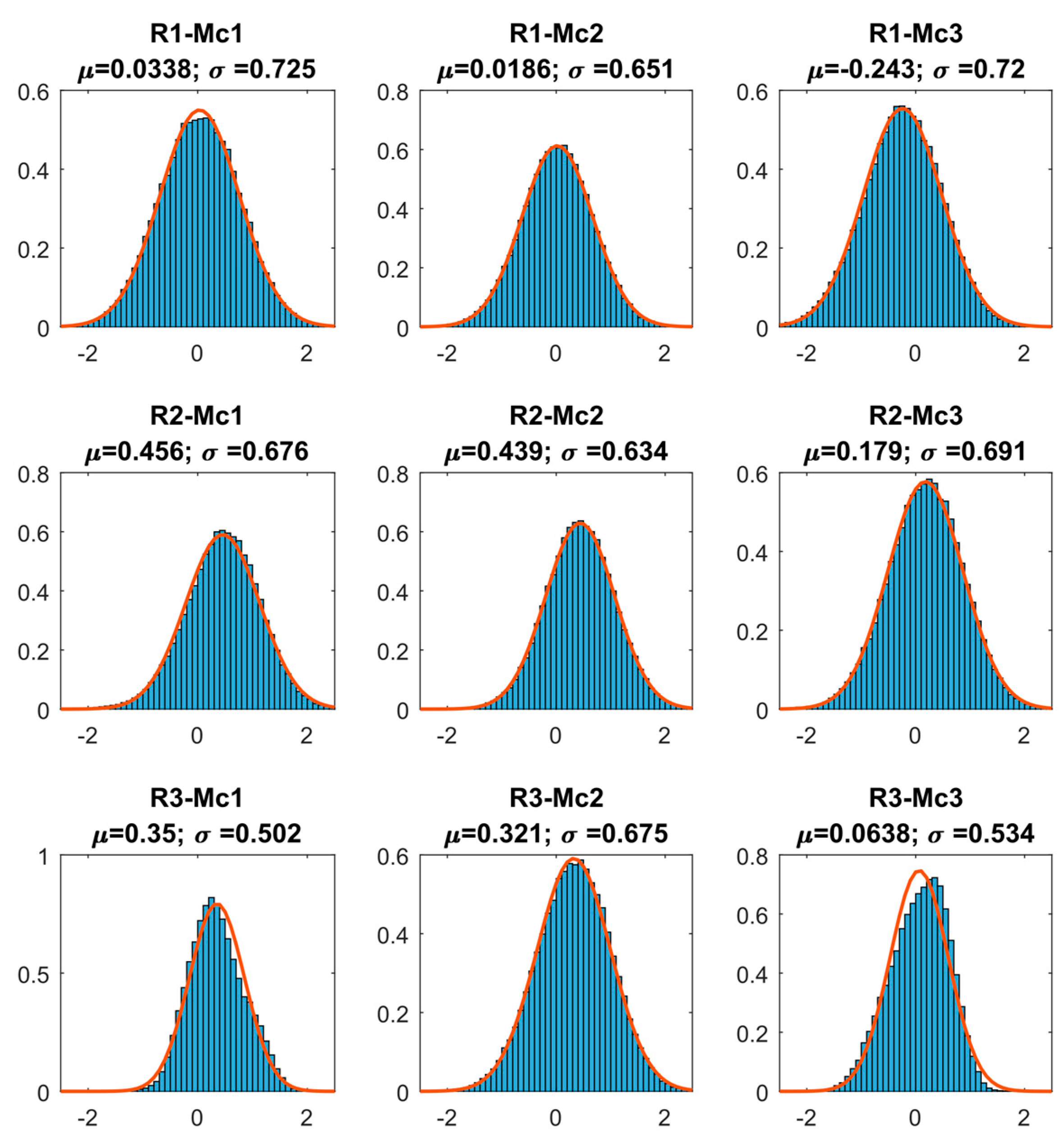
3.3. Errors Found When Scanning through a Common Mirror
The transformation matrix Kc is shown in (4). The root mean square (RMS) of the least square method was 0.00201807 m.
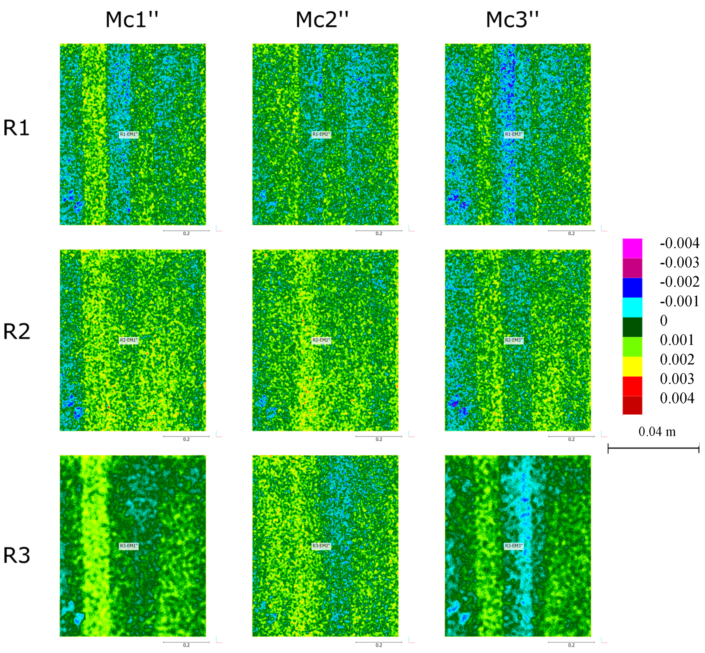
In Figure 9, the presence of the vertical band errors can be observed. Despite the use of the common mirror when scanning the reference surface, a visual inspection of the errors does not show apparently dramatic deformations compared to the previous results. Mean and standard deviations are shown in Figure 10 with the histograms of the errors. As in the previous section, the absolute minimum mean value is found in the R1-Mc1′′ case (0.03 mm). The explanation of this fact is due to the least-square adjustment of the Mc1′′ cloud to R1, which minimizes the mean. The rest of the absolute means range from 0.02 to 0.46 mm. This interval is slightly higher than the one found when using the high-quality mirrors (i.e., 0.11 to 0.36 mm). However, it is noteworthy that the order of magnitude of this error is 0.1 mm and the absolute mean error found when comparing direct scans ranged from 0.12 to 0.44 mm. This means that the absolute mean errors are under the instrumental error. The standard deviations ranged from 0.5 to 0.72 mm, which are again higher than those obtained with the direct scan but of the same order as those calculated with the high-quality mirror.
Table 1 summarizes the means and standard deviations calculated for the M3C2 distances between the compared models.
4. Discussion
4.1. Indentification of Error Sources
Different errors are expected to be found in different stages. In stage one, the point clouds R1, R2 and R3 would present only instrumental errors. Table 1 shows that the absolute mean instrumental error, when scanning an object situated closer than 10 m, ranged from 0.1 to 0.45 mm. In our case, we found that the standard deviation ranged from 0.56 to 0.59 mm. This noise is smaller than that presented in the instrument specifications, which is 2 mm at a distance of 50 m [27]. However, other studies have shown that similar instruments (Leica ScanStation P20) have an error minor than 1 mm at 50 m [9].
Additionally, this stage would also introduce deformations due to scanning through the mirrors in the analysis of points clouds Mh and Mc. Not only the deformation introduced by the mirror will appear, but other secondary issues like scratches could have an effect. Notice also that uneven mirror thickness may affect the laser time-of-flight, thus inducing errors in the measurements.
In stage two, truncation errors could be found due to the import–export process. However, this error is expected to be insignificant.
In stage three, another error could appear due to the use of the same transformation matrix for different measurements. Transformation matrices were calculated in order to minimize the error between measurement R1 with respect to Mh1′ and Mc1′; therefore, all other comparisons should have higher errors because they are not ‘optimized’. Accordingly, the absolute mean errors found in R1-Mh1′′ and R1-Mc1′′ are 0.06 and 0.03 mm. The rest of the clouds show absolute mean values from 0.02 to 0.46 mm. However, the standard deviation in all cases range between 0.5 and 0.81 and no significant differences were found between measurement number one and the rest. This means that the error for different measurements using the same transformation matrices, usually done, is not significant.
4.2. Errors Due to the Scanning through Mirrors
The scan through a high-quality mirror presented an absolute mean error that ranged from 0.06 to 0.36 mm, and its standard deviation ranged from 0.62 to 0.81 mm. However, when scanning through a common mirror, the absolute mean ranged from 0.02 to 0.46 mm, and the standard deviation ranged from 0.5 to 0.72 mm. It is observed that when using a common mirror, the absolute mean value was slightly superior to those values obtained when using a high-quality mirror most times. Surprisingly, the contrary effect was found when the standard deviation was analyzed. In this case, the standard deviation was reduced approximately by 0.1 mm.
Nevertheless, the errors obtained by comparing measurements without mirrors (R1, R2 and R3 between them) do not have significant differences to those obtained using mirrors, both in absolute value and in standard deviation. Therefore, it must be considered that the order of magnitude of the errors obtained using mirrors is under the accuracy of the instrument. As a result of this, no objective conclusion about the convenience of using one or another kind of mirror can be stated. Therefore, our results show that the use of a common mirror does not worsen the quality of the scanning with respect to the standard process under the considered conditions. Therefore, configurations introducing beam deflections are feasible and may provide accurate results without adding much complexity and cost to the system.
5. Conclusions
In this work, we presented an experimental test analyzing the feasibility of scanning a surface through a mirror in order to allow scans with truncated beams using TLS instruments. The interest of this test lies in the fact that TLS instruments cannot scan in a descending vertical direction or behind an object because of its geometry and its working principles. The test was performed in a laboratory and a whiteboard was scanned in three phases, three times per phase: direct scanning, through a high-quality mirror and through a common mirror. All scans were properly transformed and compared with the direct scanning point clouds. This analysis showed that the use of mirrors, regardless their quality, affect the noise less than the instrument error.
This work shows the possibility of scanning through a mirror with confidence when the requirements do not exceed the accuracy specifications. Future works of scanning the inside of vertical tubes will be enabled thanks to the findings presented in this work.
Acknowledgments
This work was partially funded by the University of Alicante (vigrob-157 Project, GRE14-04 Project and GRE15-19 Project), the Spanish Ministry of Economy and Competitiveness (MINECO) and EU FEDER, under Project TIN2014-55413-C2-2-P.
Author Contributions
Adrián J. Riquelme, Belén Ferrer and David Mas conceived, designed and performed the experiment; Adrián J. Riquelme analyzed the data, Adrián J. Riquelme, Belén Ferrer and David Mas wrote the paper.
Conflicts of Interest
The authors declare no conflict of interest. The founding sponsors had no role in the design of the study; in the collection, analyses, or interpretation of data; in the writing of the manuscript, and in the decision to publish the results.
References
- Slob, S. Automated Rock Mass Characterisation Using 3-D Terrestrial Laser Scannin; Delft University of Technology: Delft, The Netherlands, 2010. [Google Scholar]
- Shan, J.; Toth, C.K. Topographic Laser Ranging and Scanning: Principles and Processing; CRC Press: Boca Raton, FL, USA, 2008. [Google Scholar]
- Jaboyedoff, M.; Oppikofer, T.; Abellán, A.; Derron, M.-H.; Loye, A.; Metzger, R.; Pedrazzini, A. Use of LiDAR in landslide investigations: A review. Nat. Hazards 2012, 61, 5–28. [Google Scholar] [CrossRef]
- Thiel, K.H.; Wehr, A. Performance capabilities of laser scanners—An overview and measurement principle analysis. In Proceedings of the International Archives of Photogrammetry, Remote Sensing and Spatial Information Sciences, Istanbul, Turkey, 12–23 July 2004; Volume 36, pp. 14–18. [Google Scholar]
- Boehler, W.; Vicent, M.B.; Marbs, A. Investigating laser scanner accuracy. In Proceedings of the International Archives of Photogrammetry, Remote Sensing and Spatial Information Sciences, Dresden, Germany, 8–10 October 2003; Volume 34, pp. 696–701. [Google Scholar]
- Costantino, D.; Angelini, M.G. Qualitative and quantitative evaluation of the luminance of laser scanner radiation for the classification of materials. In Proceedings of the ISPRS-International Archives of the Photogrammetry, Remote Sensing and Spatial Information Sciences, Strasbourg, France, 2–6 September 2013; Volume 1, pp. 207–212. [Google Scholar]
- Kukko, A.; Kaasalainen, S.; Litkey, P. Effect of incidence angle on laser scanner intensity and surface data. Appl. Opt. 2008, 47, 986–992. [Google Scholar] [CrossRef] [PubMed]
- Carrea, D.; Abellán, A.; Humair, F.; Matasci, B.; Derron, M.-H.; Jaboyedoff, M. Correction of terrestrial LiDAR intensity channel using Oren–Nayar reflectance model: An application to lithological differentiation. ISPRS J. Photogramm. Remote Sens. 2016, 113, 17–29. [Google Scholar] [CrossRef]
- Wunderlich, T.; Wasmeier, P.; Ohlmann-Lauber, J.; Schäfer, T.; Reidl, F. Objective Specifications of Terrestrial Laserscanners—A Contribution of the Geodetic Laboratory at the Technische Universität München; Lehrstuhl für Geodäsie, TUM: München, Germany, 2013; ISBN 978-3-943683-21-9. [Google Scholar]
- Baltsavias, E. Airborne laser scanning: Basic relations and formulas. ISPRS J. Photogramm. Remote Sens. 1999, 54, 199–214. [Google Scholar] [CrossRef]
- Wehr, A.; Lohr, U. Airborne laser scanning—An introduction and overview. ISPRS J. Photogramm. Remote Sens. 1999, 54, 68–82. [Google Scholar] [CrossRef]
- Pu, S.; Rutzinger, M.; Vosselman, G.; Oude Elberink, S. Recognizing basic structures from mobile laser scanning data for road inventory studies. ISPRS J. Photogramm. Remote Sens. 2011, 66, S28–S39. [Google Scholar] [CrossRef]
- Liang, X.; Kukko, A.; Kaartinen, H.; Hyyppä, J.; Yu, X.; Jaakkola, A.; Wang, Y. Possibilities of a Personal Laser Scanning System for Forest Mapping and Ecosystem Services. Sensors 2014, 14, 1228–1248. [Google Scholar] [CrossRef] [PubMed]
- Liang, X.; Kankare, V.; Hyyppä, J.; Wang, Y.; Kukko, A.; Haggrén, H.; Yu, X.; Kaartinen, H.; Jaakkola, A.; Guan, F.; et al. Terrestrial laser scanning in forest inventories. ISPRS J. Photogramm. Remote Sens. 2016, 115, 63–77. [Google Scholar] [CrossRef]
- Kukko, A.; Kaartinen, H.; Hyyppä, J.; Chen, Y. Multiplatform Mobile Laser Scanning: Usability and Performance. Sensors 2012, 12, 11712–11733. [Google Scholar] [CrossRef]
- Alho, P.; Kukko, A.; Hyyppä, H.; Kaartinen, H.; Hyyppä, J.; Jaakkola, A. Application of boat-based laser scanning for river survey. Earth Surf. Process. Landf. 2009, 34, 1831–1838. [Google Scholar] [CrossRef]
- Abellán, A.; Derron, M.-H.; Jaboyedoff, M. ‘Use of 3D Point Clouds in Geohazards’ Special Issue: Current Challenges and Future Trends. Remote Sens. 2016, 8, 130. [Google Scholar] [CrossRef]
- McKinion, J.M.; Willers, J.L.; Jenkins, J.N. Comparing high density LIDAR and medium resolution GPS generated elevation data for predicting yield stability. Comput. Electron. Agric. 2010, 74, 244–249. [Google Scholar] [CrossRef]
- Johnson, K.M.; Ouimet, W.B. Rediscovering the lost archaeological landscape of southern New England using airborne light detection and ranging (LiDAR). J. Archaeol. Sci. 2014, 43, 9–20. [Google Scholar] [CrossRef]
- Levinson, J.; Askeland, J.; Becker, J.; Dolson, J.; Held, D.; Kammel, S.; Kolter, J.Z.; Langer, D.; Pink, O.; Pratt, V.; et al. Towards fully autonomous driving: Systems and algorithms. In Proceedings of the 2011 IEEE Intelligent Vehicles Symposium (IV), Baden-Baden, Germany, 5–9 June 2011; IEEE: Piscataway, NJ, USA, 2011; pp. 163–168. [Google Scholar]
- Amzajerdian, F.; Pierrottet, D.; Petway, L.; Hines, G.; Roback, V. Lidar systems for precision navigation and safe landing on planetary bodies. In Proceedings of the 2011-International Symposium on Photoelectronic Detection and Imaging, Beijing, China, 24–26 May 2011; Volume 8192, p. 819202. [Google Scholar]
- Matasci, B.; Carrea, D.; Abellán, A.; Derron, M.H.; Humair, F.; Jaboyedoff, M.; Metzger, R. Geological mapping and fold modeling using terrestrial laser scanning point clouds: Application to the Dents-du-Midi limestone massif (Switzerland). Eur. J. Remote Sens. 2015, 48, 569–591. [Google Scholar] [CrossRef]
- Lato, M.J.; Diederichs, M.S. Mapping shotcrete thickness using LiDAR and photogrammetry data: Correcting for over-calculation due to rockmass convergence. Tunn. Undergr. Space Technol. 2014, 41, 234–240. [Google Scholar] [CrossRef]
- Abellán, A.; Oppikofer, T.; Jaboyedoff, M.; Rosser, N.J.; Lim, M.; Lato, M.J. Terrestrial laser scanning of rock slope instabilities. Earth Surf. Process. Landf. 2014, 39, 80–97. [Google Scholar] [CrossRef]
- Yang, S.-W.; Wang, C.-C. On Solving Mirror Reflection in LIDAR Sensing. IEEE/ASME Trans. Mechatron. 2011, 16, 255–265. [Google Scholar] [CrossRef]
- Fasano, A.; Callieri, M.; Cignoni, P.; Scopigno, R. Exploiting mirrors for laser stripe 3D scanning. In Proceedings of the International Conference on 3-D Digital Imaging and Modeling, 3DIM, Banff, AB, Canada, 6–10 October 2003; IEEE: Piscataway, NJ, USA, 2003; pp. 243–250. [Google Scholar]
- Leica Geosystems AG. Leica ScanStation C10 Data Sheet; Leica Geosystems AG: Heerbrugg, Switzerland, 2011. [Google Scholar]
- Reshetouski, I.; Ihrke, I. Mirrors in computer graphics, computer vision and time-of-flight imaging. In Time-of-Flight and Depth Imaging. Sensors, Algorithms, and Applications; Springer: Berlin, Germany, 2013; pp. 77–104. [Google Scholar]
- Leica Cyclone v9.1 2016. Available online: http://hds.leica-geosystems.com/en/Support-Downloads-Cyclone-Downloads_27054.htm (accessed on 9 November 2017).
- Lague, D.; Brodu, N.; Leroux, J.J. Accurate 3D comparison of complex topography with terrestrial laser scanner: Application to the Rangitikei canyon (NZ). ISPRS J. Photogramm. Remote Sens. 2013, 82, 10–26. [Google Scholar] [CrossRef]
Figure 1.
(a) Horizontal and vertical field-of-view of a 3D laser scanner (3DLS) model Leica C10; (b) example of a full scan using that scanner, where the area under the scanner cannot be captured. Images of the 3DLS modified from www.leica-geosystems.com.
Figure 1.
(a) Horizontal and vertical field-of-view of a 3D laser scanner (3DLS) model Leica C10; (b) example of a full scan using that scanner, where the area under the scanner cannot be captured. Images of the 3DLS modified from www.leica-geosystems.com.

Figure 2.
Laboratory where the test is conducted. (a) Scheme of the laboratory and location of the TLS, the mirror and the scanned whiteboard; (b) bubble view of the 3D point cloud centered in the TLS scan station.
Figure 2.
Laboratory where the test is conducted. (a) Scheme of the laboratory and location of the TLS, the mirror and the scanned whiteboard; (b) bubble view of the 3D point cloud centered in the TLS scan station.

Figure 3.
Scanned whiteboard, with four black and white targets. The area of interest is between the four targets, and the albedo is approximately 50%.
Figure 3.
Scanned whiteboard, with four black and white targets. The area of interest is between the four targets, and the albedo is approximately 50%.

Figure 4.
Flowchart of the methodology.

Figure 5.
Multiscale Model to Model Cloud Comparison (M3C2) distance of the self-compared point clouds for direct scanning (R1, R2 and R3). (a) Distances between clouds R1 and R2; (b) distances between clouds R1 and R3 and (c) distances between clouds R2 and R3.
Figure 5.
Multiscale Model to Model Cloud Comparison (M3C2) distance of the self-compared point clouds for direct scanning (R1, R2 and R3). (a) Distances between clouds R1 and R2; (b) distances between clouds R1 and R3 and (c) distances between clouds R2 and R3.

Figure 6.
Histograms and fit of the normal probability distribution to the calculated errors in Figure 5. Units are shown in mm.
Figure 6.
Histograms and fit of the normal probability distribution to the calculated errors in Figure 5. Units are shown in mm.

Figure 7.
M3C2 distance of the compared point clouds: direct scanning (R1, R2 and R3) with scanning through a high-quality mirror (Mh1′′, Mh2′′ and Mh3′′).
Figure 7.
M3C2 distance of the compared point clouds: direct scanning (R1, R2 and R3) with scanning through a high-quality mirror (Mh1′′, Mh2′′ and Mh3′′).

Figure 8.
Histograms and fit of the normal probability distribution to the calculated errors of Figure 7. Units are shown in mm.
Figure 8.
Histograms and fit of the normal probability distribution to the calculated errors of Figure 7. Units are shown in mm.

Figure 9.
M3C2 distance of the compared point clouds: direct scanning (R1, R2 and R3) with scanning through a common mirror (Mc1′′, Mc2′′ and Mc3′′).
Figure 9.
M3C2 distance of the compared point clouds: direct scanning (R1, R2 and R3) with scanning through a common mirror (Mc1′′, Mc2′′ and Mc3′′).

Figure 10.
Histograms and fit of the normal probability distribution to the calculated errors of Figure 9.
Figure 10.
Histograms and fit of the normal probability distribution to the calculated errors of Figure 9.


Table 1.
Mean and standard deviation of the comparison between point clouds in mm.
| Compared to | R1 | R2 | R3 |
|---|---|---|---|
| Mh1′′ | −0.06/0.81 | 0.36/0.76 | 0.25/0.67 |
| Mh2′′ | −0.2/0.8 | 0.23/0.67 | 0.11/0.79 |
| Mh3′′ | −0.16/0.74 | 0.26/0.68 | 0.11/0.62 |
| Mc1′′ | 0.03/0.72 | 0.46/0.68 | 0.35/0.5 |
| Mc2′′ | 0.02/0.65 | 0.44/0.63 | 0.32/0.68 |
| Mc3′′ | −0.24/0.72 | 0.18/0.69 | 0.06/0.53 |
| R1 | - | −0.44/0.59 | −0.31/0.58 |
| R2 | −0.44/0.59 | - | 0.12/0.56 |
| R3 | −0.31/0.58 | 0.12/0.56 | - |
© 2017 by the authors. Licensee MDPI, Basel, Switzerland. This article is an open access article distributed under the terms and conditions of the Creative Commons Attribution (CC BY) license (http://creativecommons.org/licenses/by/4.0/).
Share and Cite
MDPI and ACS Style
Riquelme, A.J.; Ferrer, B.; Mas, D. Use of High-Quality and Common Commercial Mirrors for Scanning Close-Range Surfaces Using 3D Laser Scanners: A Laboratory Experiment. Remote Sens. 2017, 9, 1152. https://doi.org/10.3390/rs9111152
AMA Style
Riquelme AJ, Ferrer B, Mas D. Use of High-Quality and Common Commercial Mirrors for Scanning Close-Range Surfaces Using 3D Laser Scanners: A Laboratory Experiment. Remote Sensing. 2017; 9(11):1152. https://doi.org/10.3390/rs9111152
Chicago/Turabian StyleRiquelme, Adrián J., Belén Ferrer, and David Mas. 2017. "Use of High-Quality and Common Commercial Mirrors for Scanning Close-Range Surfaces Using 3D Laser Scanners: A Laboratory Experiment" Remote Sensing 9, no. 11: 1152. https://doi.org/10.3390/rs9111152
Note that from the first issue of 2016, this journal uses article numbers instead of page numbers. See further details here.