
Development of Kinematic 3D Laser Scanning System for Indoor Mapping and As-Built BIM Using Constrained SLAM

Abstract
:1. Introduction
2. Methods
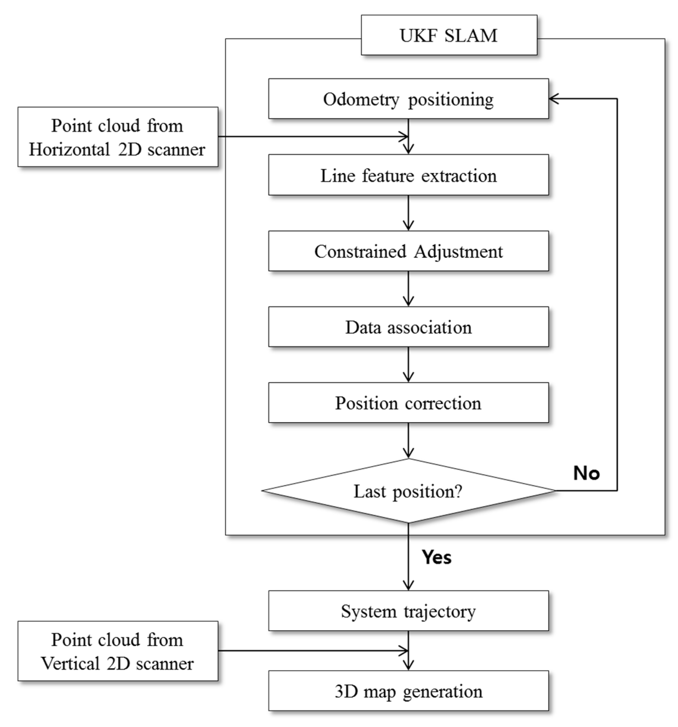
2.1. Overview

2.2. Odometry Positioning
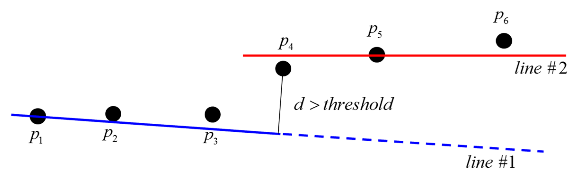
2.3. Line-Feature Extraction

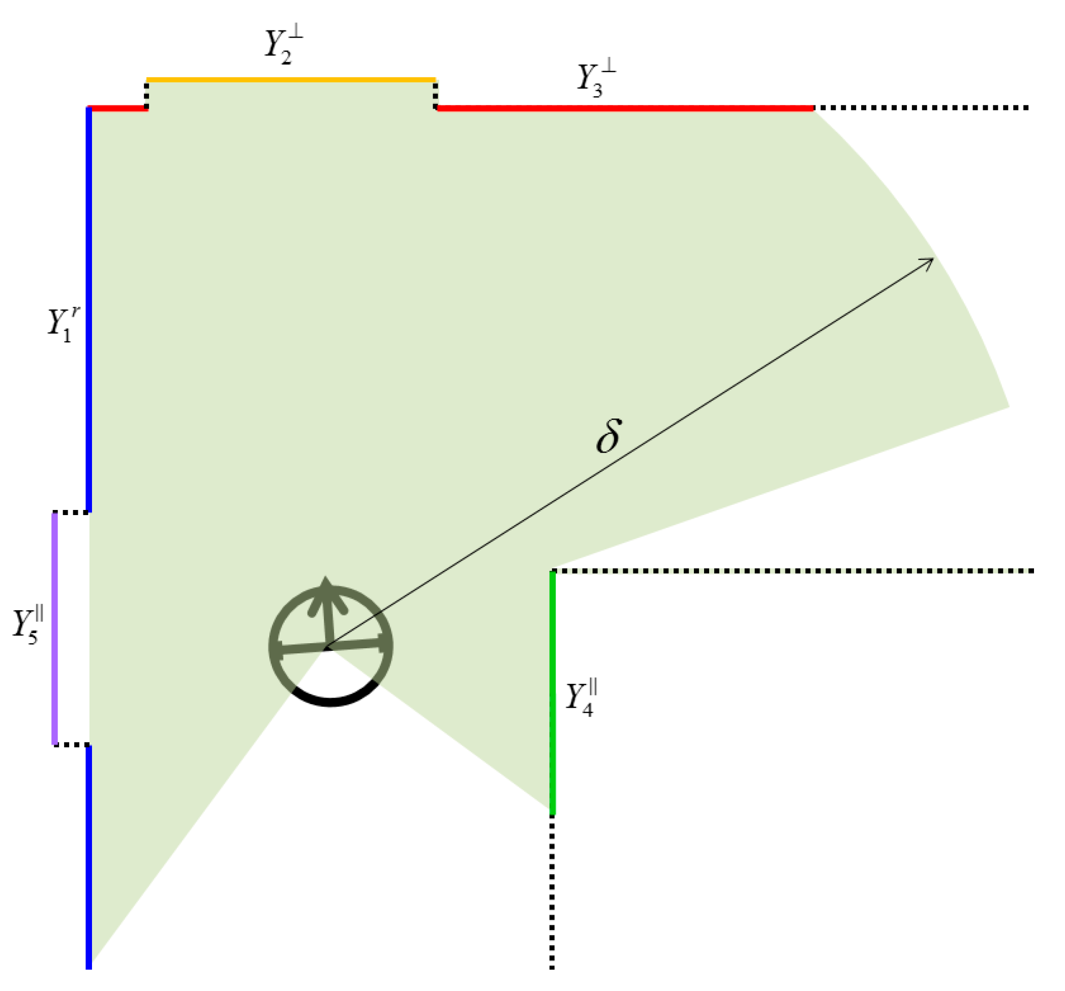
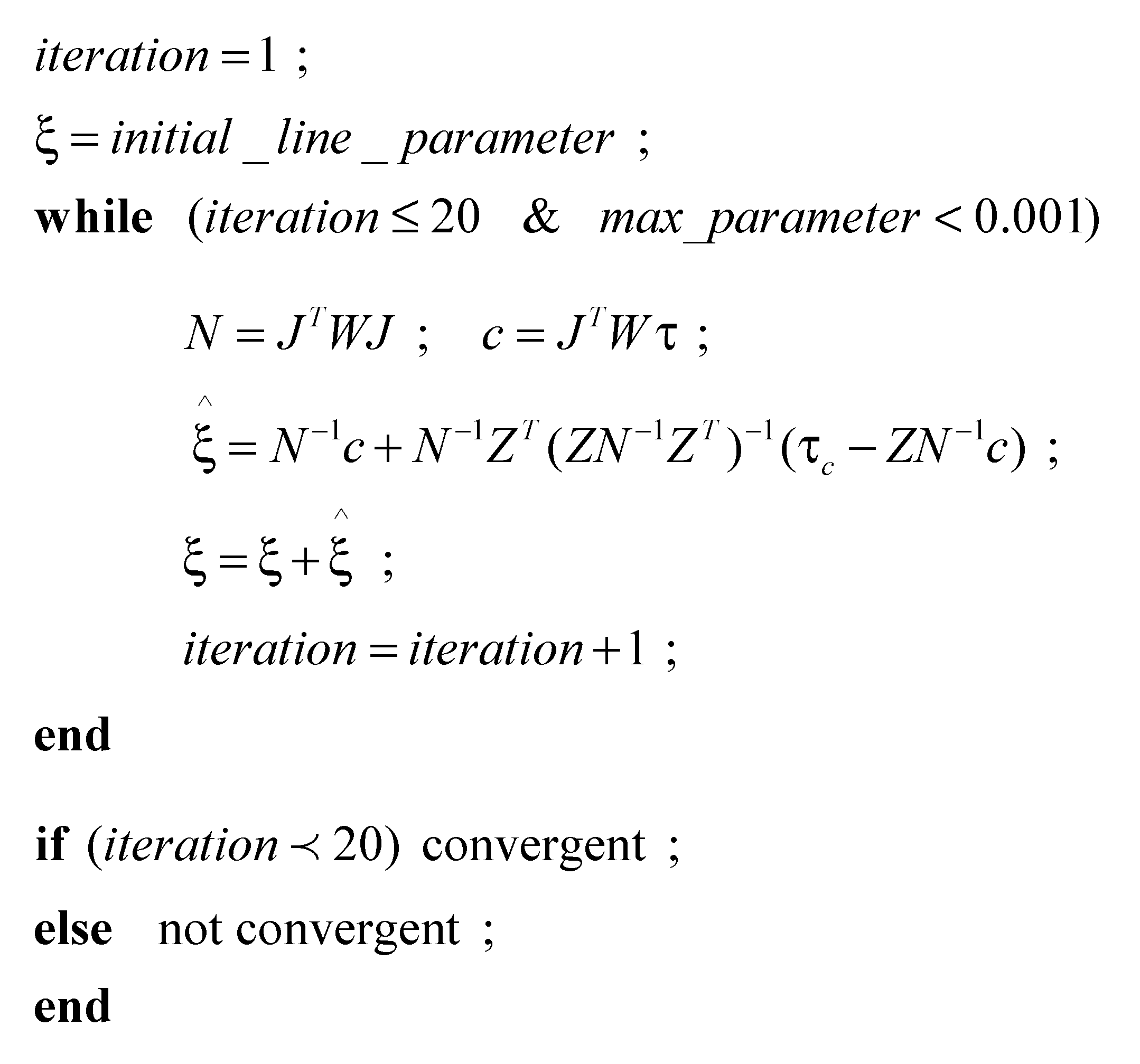
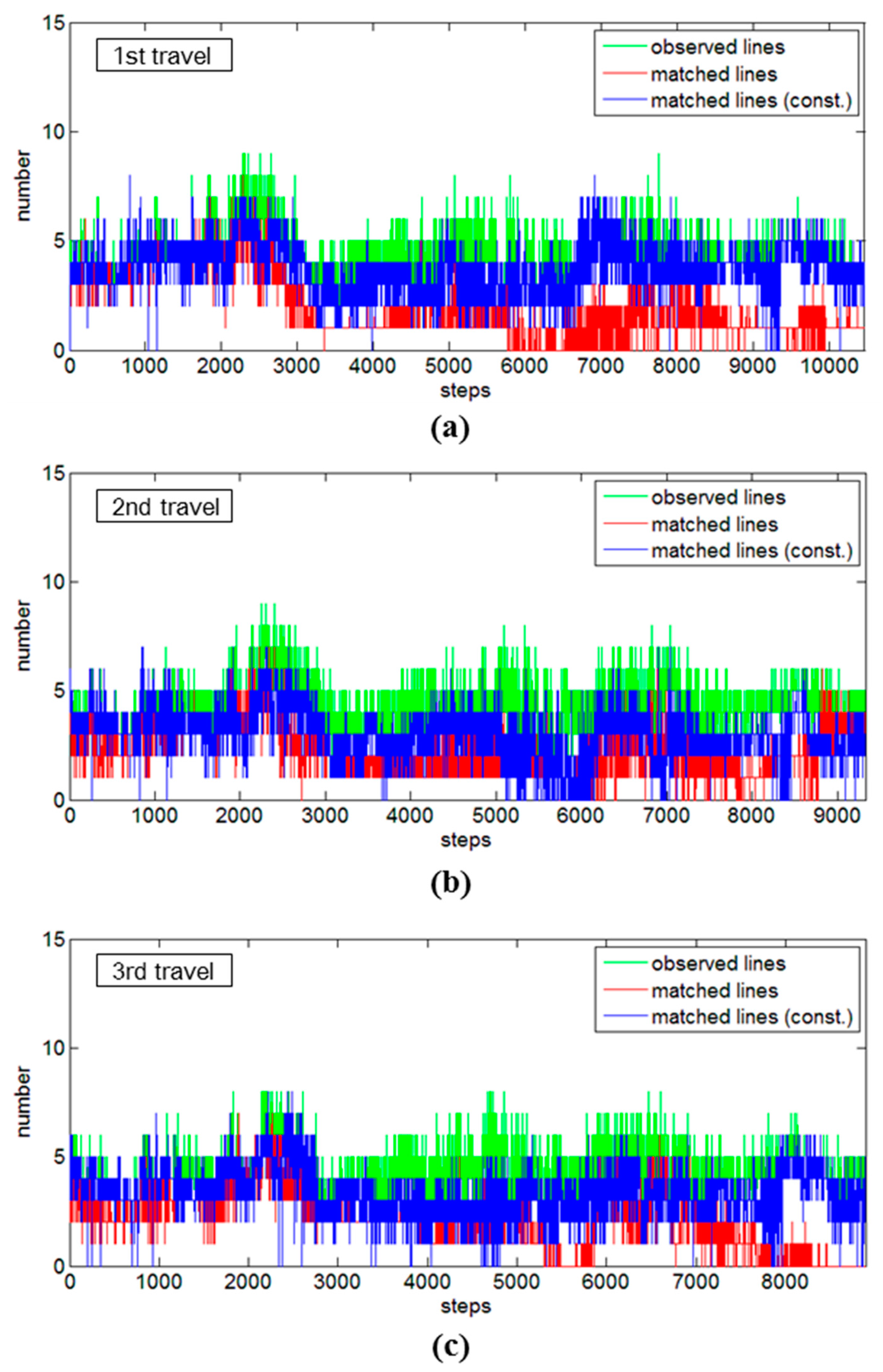
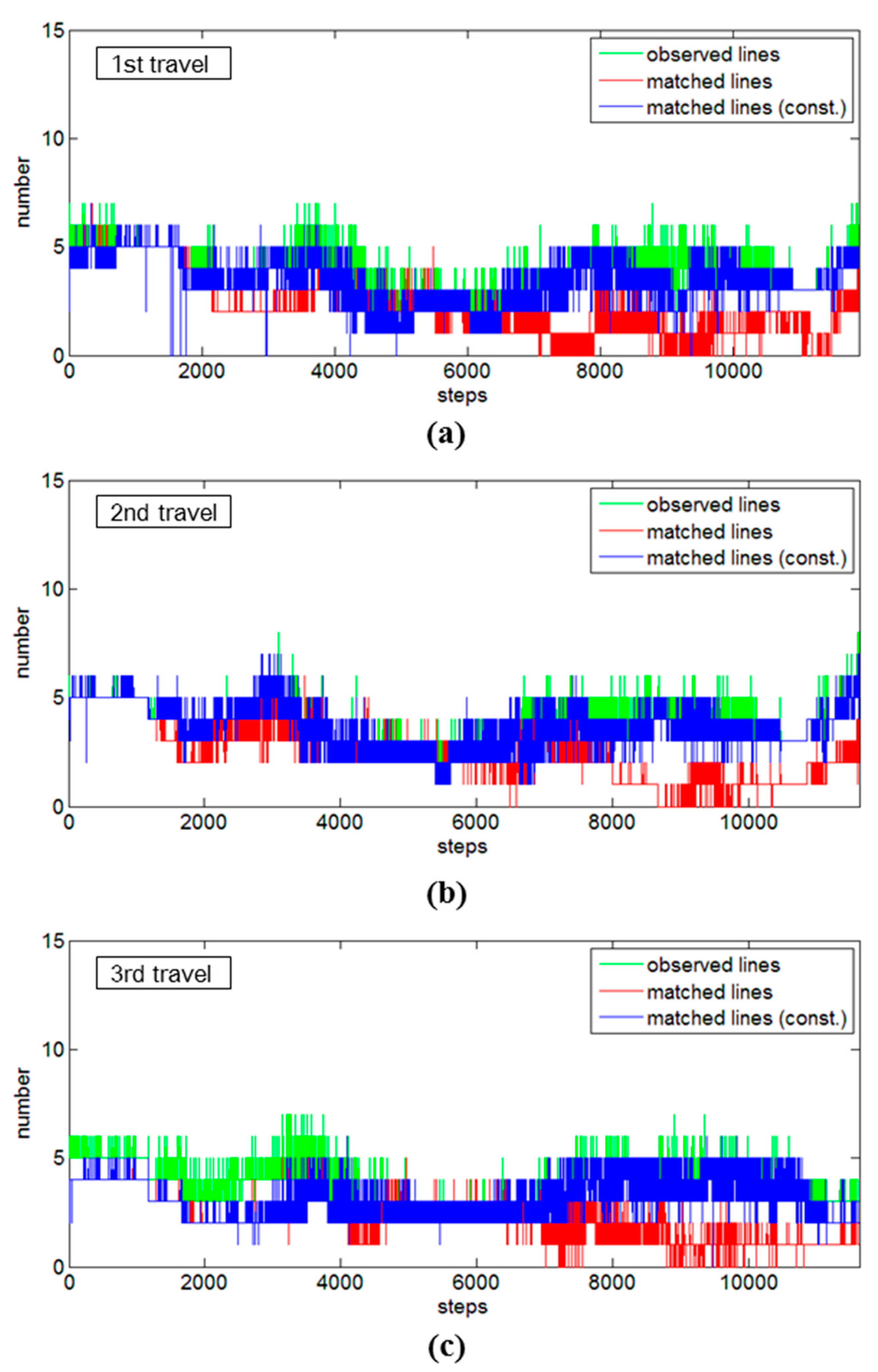
2.4. Constrained Adjustment


2.5. Data Association
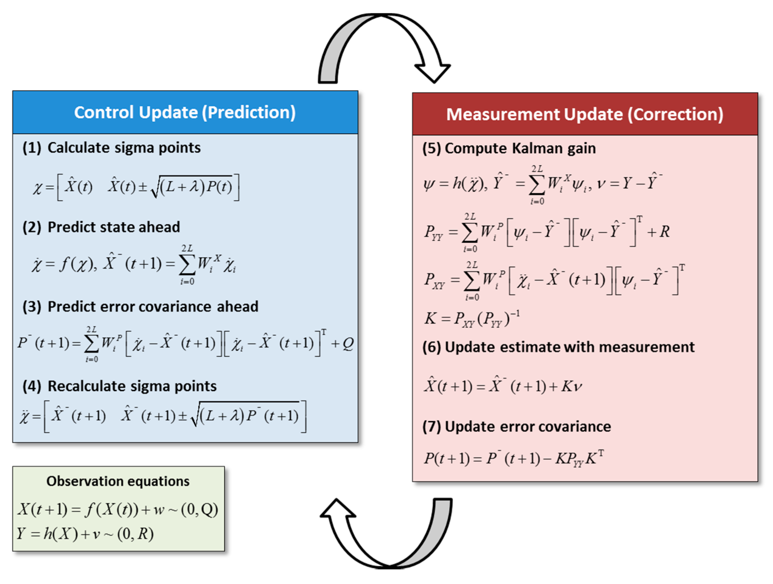
2.6. Unscented Kalman Filter

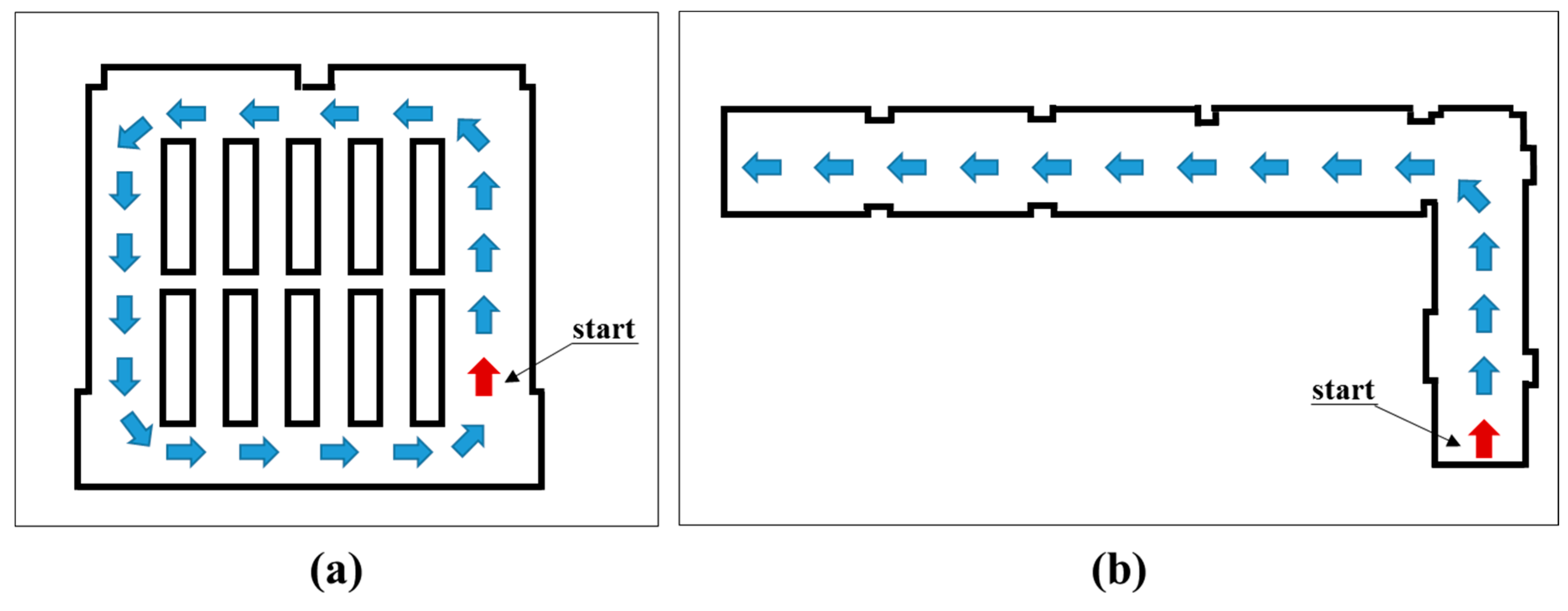
3. Experimental Results
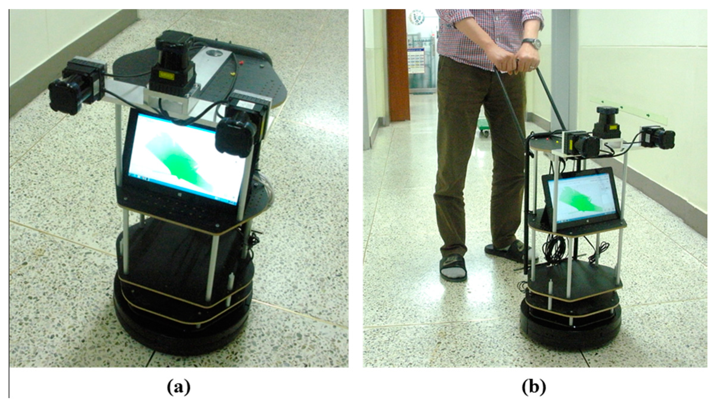
3.1. Implementation of Kinematic Scanning System


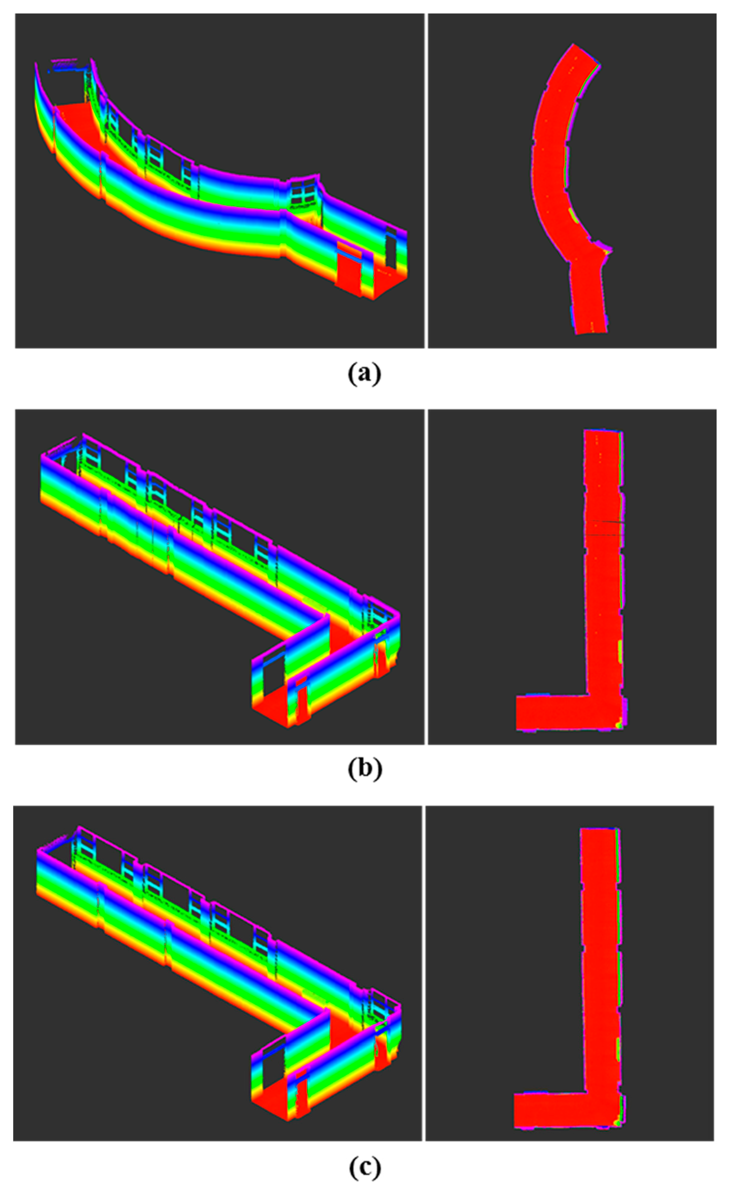
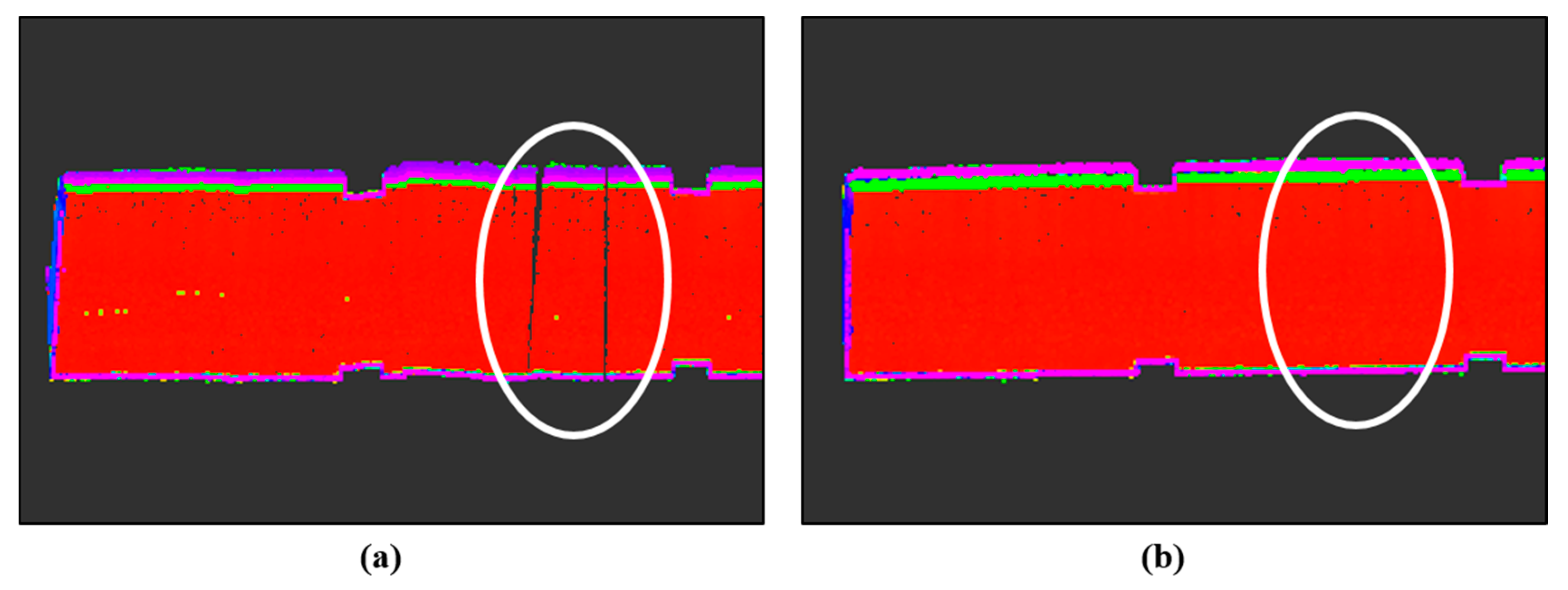
3.2. Visualization of Point-Cloud Data


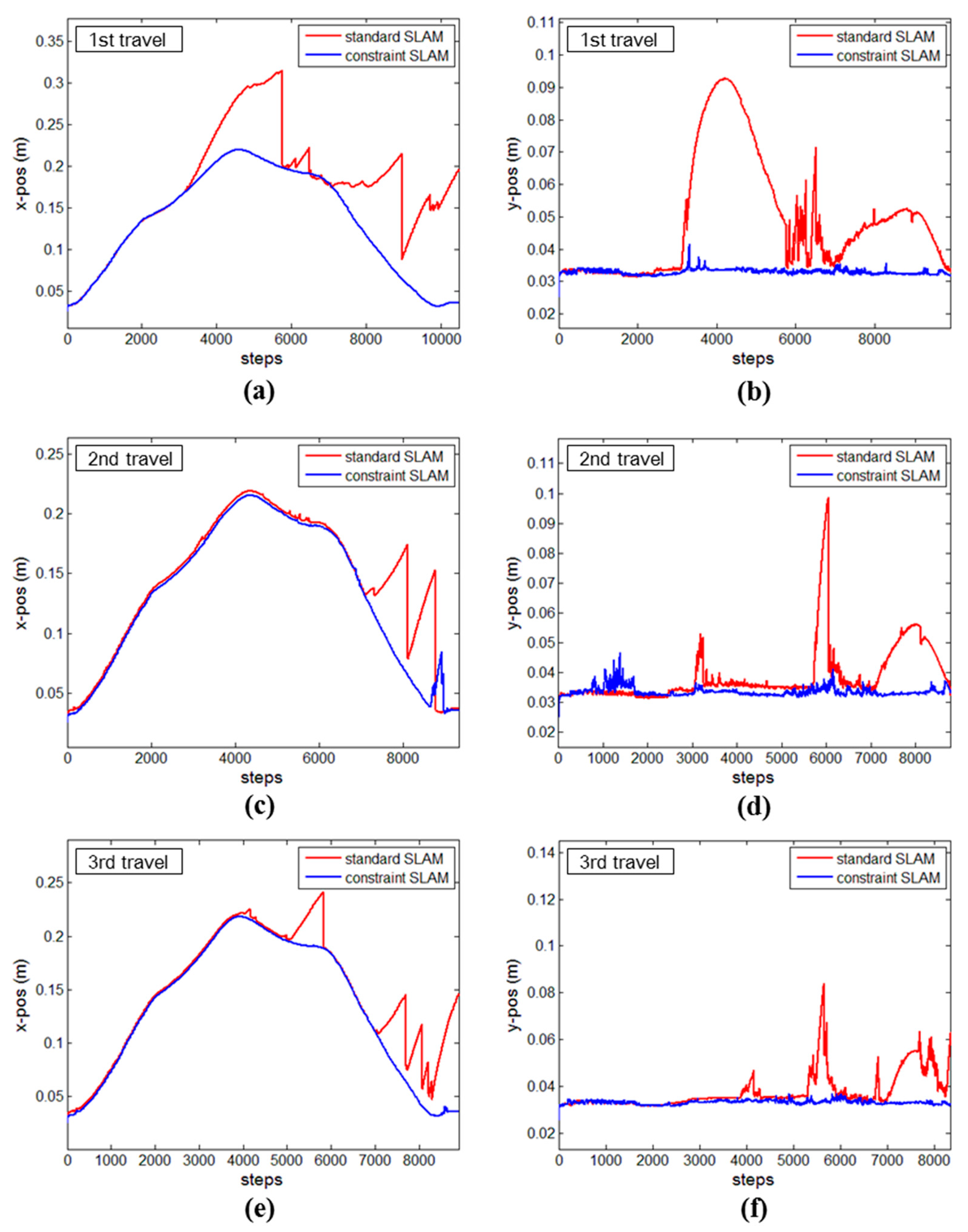
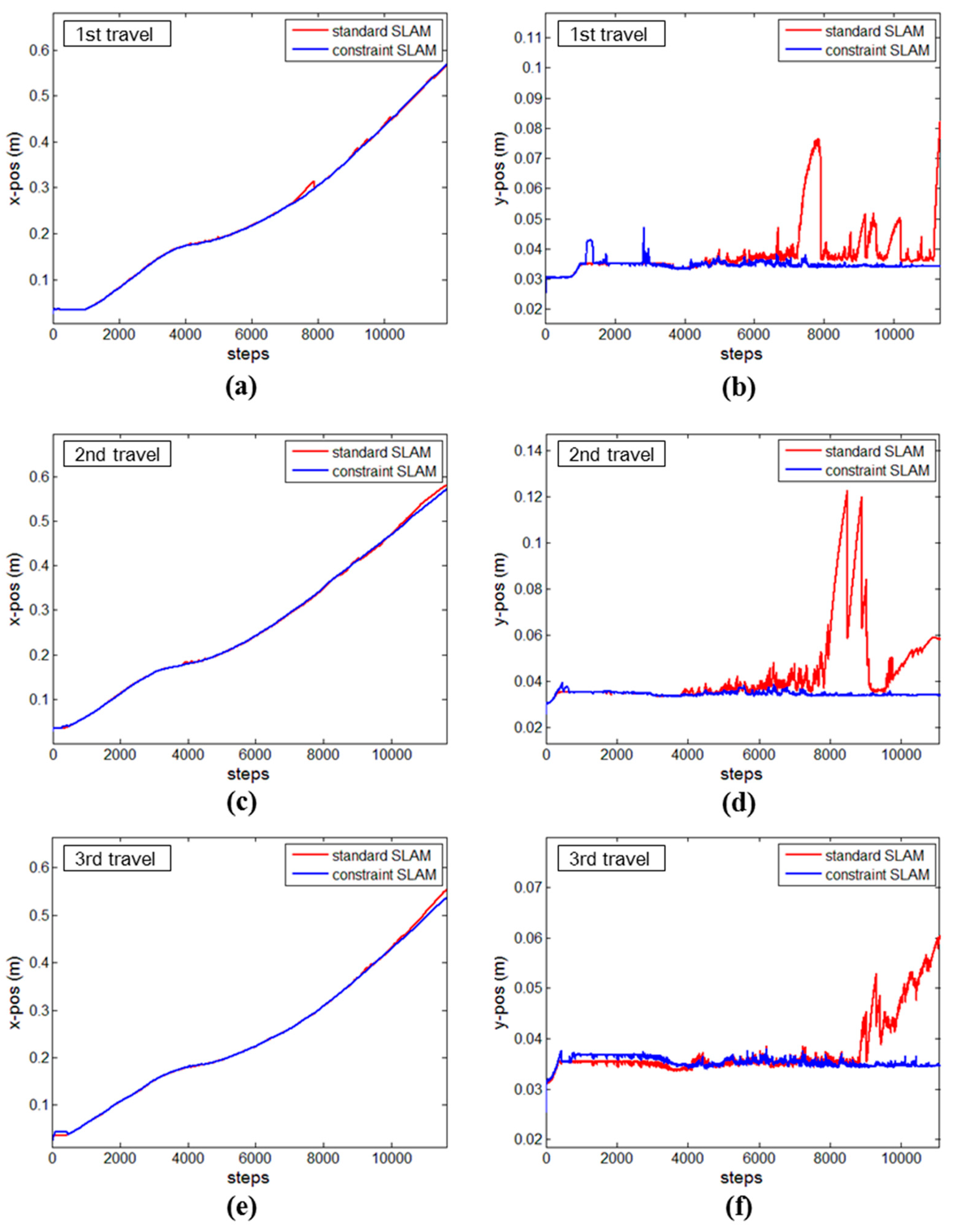
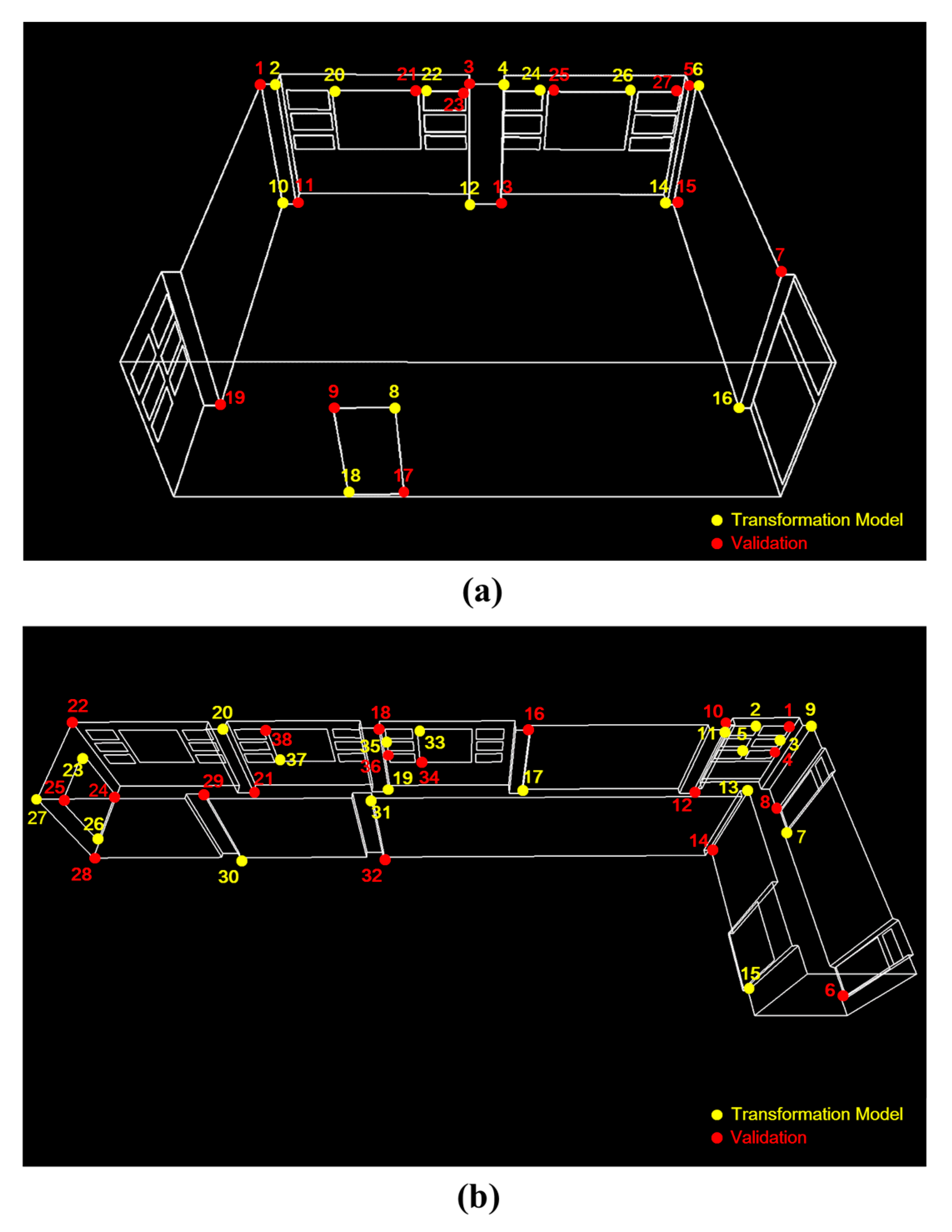
3.3. Accuracy Assessment


| Point ID | Error Vector X | Error Vector Y | Error Vector Z | Error |
|---|---|---|---|---|
| 1 | −0.021 | −0.013 | 0.005 | 0.025 |
| 3 | −0.023 | 0.000 | −0.013 | 0.027 |
| 5 | 0.003 | −0.006 | −0.015 | 0.016 |
| 7 | 0.010 | 0.061 | 0.021 | 0.066 |
| 9 | 0.030 | −0.015 | −0.013 | 0.036 |
| 11 | −0.019 | 0.030 | 0.022 | 0.042 |
| 13 | −0.021 | 0.013 | 0.002 | 0.025 |
| 15 | 0.018 | 0.001 | 0.017 | 0.025 |
| 17 | 0.022 | −0.011 | −0.001 | 0.025 |
| 19 | 0.031 | 0.009 | −0.008 | 0.034 |
| 21 | 0.000 | 0.000 | −0.004 | 0.004 |
| 23 | 0.007 | −0.014 | 0.008 | 0.018 |
| 25 | 0.041 | 0.004 | −0.001 | 0.041 |
| 27 | 0.029 | −0.045 | −0.002 | 0.053 |
| Average error | 0.034 | |||
| RMSE | 0.024 | 0.024 | 0.012 | 0.036 |
| SAS | 0.050 |
| Point ID | Error Vector X | Error Vector Y | Error Vector Z | Error |
|---|---|---|---|---|
| 1 | −0.031 | 0.009 | 0.000 | 0.032 |
| 4 | −0.059 | 0.019 | −0.002 | 0.062 |
| 6 | −0.062 | 0.023 | 0.022 | 0.069 |
| 8 | −0.010 | 0.003 | 0.017 | 0.020 |
| 10 | −0.013 | −0.015 | 0.004 | 0.020 |
| 12 | 0.014 | 0.014 | −0.034 | 0.039 |
| 14 | −0.002 | 0.036 | −0.039 | 0.053 |
| 16 | 0.011 | 0.025 | 0.011 | 0.030 |
| 18 | 0.007 | −0.012 | 0.006 | 0.015 |
| 21 | 0.010 | −0.024 | 0.007 | 0.026 |
| 22 | 0.008 | −0.027 | −0.007 | 0.029 |
| 24 | 0.016 | −0.046 | −0.011 | 0.050 |
| 25 | 0.056 | −0.026 | −0.002 | 0.062 |
| 28 | −0.007 | −0.033 | −0.001 | 0.034 |
| 29 | 0.027 | −0.010 | −0.009 | 0.030 |
| 32 | 0.019 | −0.025 | −0.012 | 0.034 |
| 34 | 0.088 | −0.022 | −0.005 | 0.090 |
| 36 | −0.002 | −0.037 | 0.015 | 0.040 |
| 38 | −0.063 | −0.026 | 0.053 | 0.086 |
| Average error | 0.043 | |||
| RMSE | 0.036 | 0.025 | 0.019 | 0.048 |
| SAS | 0.067 |
4. Conclusions
Acknowledgments
Author Contributions
Conflicts of Interest
References
- Turkan, Y.; Bosche, F.; Haas, C.T.; Haas, R. Towards automated progress tracking of erection of concrete structures. In Proceedings of the 6th International Conference on Innovation in Architecture, Engineering & Construction (AEC’10), State College, PA, USA, 9–11 June 2010.
- Anil, E.B.; Akinci, B.; Huber, D. Representation requirements of as-is building information models generated from laser scanned point cloud data. In Proceedings of the International Symposium on Automation and Robotics in Construction (ISARC), Seoul, Korea, 29 June–2 July 2011.
- Han, S.; Cho, H.; Kim, S.; Jung, J.; Heo, J. Automated and efficient method for extraction of tunnel cross sections using terrestrial laser scanned data. J. Comput. Civil Eng. 2012, 27, 274–281. [Google Scholar] [CrossRef]
- Randall, T. Construction engineering requirements for integrating laser scanning technology and building information modeling. J. Construct. Eng. Manag. 2011, 137, 797–805. [Google Scholar] [CrossRef]
- Heo, J.; Jeong, S.; Park, H.K.; Jung, J.; Han, S.; Hong, S.; Sohn, H.G. Productive high-complexity 3D city modeling with point clouds collected from terrestrial lidar. Comput. Environ. Urban Syst. 2013, 41, 26–38. [Google Scholar] [CrossRef]
- Tang, P.; Huber, D.; Akinci, B.; Lipman, R.; Lytle, A. Automatic reconstruction of as-built building information models from laser-scanned point clouds: A review of related techniques. Autom. Construct. 2010, 19, 829–843. [Google Scholar] [CrossRef]
- Jung, J.; Hong, S.; Jeong, S.; Kim, S.; Cho, H.; Hong, S.; Heo, J. Productive modeling for development of as-built bim of existing indoor structures. Autom. Construct. 2014, 42, 68–77. [Google Scholar] [CrossRef]
- Volk, R.; Stengel, J.; Schultmann, F. Building information modeling (BIM) for existing buildings—Literature review and future needs. Autom. Construct. 2014, 38, 109–127. [Google Scholar] [CrossRef]
- Pătrăucean, V.; Armeni, I.; Nahangi, M.; Yeung, J.; Brilakis, I.; Haas, C. State of research in automatic as-built modelling. Adv. Eng. Inf. 2015, 29, 162–171. [Google Scholar] [CrossRef]
- Becerik-Gerber, B.; Jazizadeh, F.; Kavulya, G.; Calis, G. Assessment of target types and layouts in 3D laser scanning for registration accuracy. Autom. Construct. 2011, 20, 649–658. [Google Scholar] [CrossRef]
- Arayici, Y. Towards building information modelling for existing structures. Struct. Surv. 2008, 26, 210–222. [Google Scholar] [CrossRef]
- Campbell, D.; Whitty, M.; Lim, S. Mobile 3D indoor mapping using the continuous normal distributions transform. In Proceedings of the 2012 International Conference on Indoor Positioning and Indoor Navigation (IPIN), Sydney, Australia, 13–15 November 2012; pp. 1–9.
- Hähnel, D.; Burgard, W.; Thrun, S. Learning compact 3D models of indoor and outdoor environments with a mobile robot. Robot. Auton. Syst. 2003, 44, 15–27. [Google Scholar] [CrossRef]
- Weingarten, J.; Gruener, G.; Siegwart, R. A fast and robust 3D feature extraction algorithm for structured environment reconstruction. In Proceediings of the 11th International Conference on Advanced Robotics (ICAR), Coimbra, Portugal, 30 June–3 July 2003.
- Nuchter, A.; Surmann, H.; Hertzberg, J. Automatic model refinement for 3D reconstruction with mobile robots. In Proceedings of the 2003 IEEE 4th International Conference on 3D Digital Imaging and Modeling (3DIM), Banff, AB, Canada, 6–10 October 2003; pp. 394–401.
- Wang, Y.; Huo, J.; Wang, X. A real-time robotic indoor 3D mapping system using duel 2D laser range finders. In Proceedings of the 2014 33rd Chinese Control Conference (CCC), Nanjing, China, 28–30 July 2014; pp. 8542–8546.
- Yan, R.J.; Wu, J.; Lee, J.Y.; Han, C.S. 3D point cloud map construction based on line segments with two mutually perpendicular laser sensors. In Proceedings of the International Conference on Control, Automation and Systems (ICCAS), Kimdaejung Convention Center, Gwangju, Korea, 20–23 October 2013; pp. 1114–1116.
- Folkesson, J.; Christensen, H. Graphical SLAM-A self-correcting map. In Proceedings of the 2004 IEEE International Conference on Robotics and Automation (ICRA), New Orleans, LA, USA, 26 April–1 May 2004; pp. 383–390.
- Arras, K.O.; Castellanos, J.A.; Schilt, M.; Siegwart, R. Feature-based multi-hypothesis localization and tracking using geometric constraints. Robot. Auton. Syst. 2003, 44, 41–53. [Google Scholar] [CrossRef]
- Lee, K.W.; Wijesoma, S.; Guzmán, J.I. A constrained SLAM approach to robust and accurate localisation of autonomous ground vehicles. Robot. Auton. Syst. 2007, 55, 527–540. [Google Scholar] [CrossRef]
- Zunino, G. Simultaneous localization and mapping for navigation in realistic environments. Avaliable online: https://www.nada.kth.se/utbildning/forsk.utb/avhandlingar/lic/020220.pdf (accessed on 5 July 2015).
- Nguyen, V.; Harati, A.; Martinelli, A.; Siegwart, R.; Tomatis, N. Orthogonal SLAM: A step toward lightweight indoor autonomous navigation. In Proceedings of the 2006 IEEE/RSJ International Conference on Intelligent Robots and Systems (IROS), Beijing, China, 10–15 October 2006; pp. 5007–5012.
- Choi, Y.H.; Lee, T.K.; Oh, S.Y. A line feature based SLAM with low grade range sensors using geometric constraints and active exploration for mobile robot. Auton. Robots 2008, 24, 13–27. [Google Scholar] [CrossRef]
- Kuo, B.W.; Chang, H.H.; Chen, Y.C.; Huang, S.Y. A light-and-fast SLAM algorithm for robots in indoor environments using line segment map. J. Robot. 2011, 2011. [Google Scholar] [CrossRef]
- Choi, H.; Kim, R.; Kim, E. An efficient ceiling-view SLAM using relational constraints between landmarks. Int. J. Adv. Robot. Syst. 2014, 11, 1–11. [Google Scholar] [CrossRef]
- Wolf, P.R.; Ghilani, C.D. Adjustment Computations: Statistics and Least Squares in Surveying and GIS; John Wiley & Sons: New York, NY, USA, 1997. [Google Scholar]
- Snow, K. Adjustment Computation Notes; The Ohio State University: Columbus, OH, USA, 2009; p. 92. [Google Scholar]
- Weingarten, J. Feature-Based 3D SLAM; Swiss Federal Institute of Technology Lausanne: Lausanne, Switzerland, 2006. [Google Scholar]
- Wang, H.; Fu, G.; Li, J.; Yan, Z.; Bian, X. An adaptive UKF based SLAM method for unmanned underwater vehicle. Math. Probl. Eng. 2013, 2013. [Google Scholar] [CrossRef]
- General Services Administration. Bim Guide for 3D Imaging, ver. 1.0; U.S. General Services Administration: Washington, DC, USA, 2009; p. 53. [Google Scholar]
- Garulli, A.; Giannitrapani, A.; Rossi, A.; Vicino, A. Mobile robot SLAM for line-based environment representation. In Proceedings of the 44th IEEE Conference on Decision and Control, and 2005 European Control Conference (CDC-ECC), Seville, Spain, 12–15 December 2005; pp. 2041–2046.
- An, S.Y.; Kang, J.G.; Lee, L.K.; Oh, S.Y. SLAM with salient line feature extraction in indoor environments. In Proceedings of the 2010 11th International Conference on Control Automation Robotics & Vision (ICARCV), Singapore, 7–10 December 2010; pp. 410–416.
- Yap, T.N.; Shelton, C.R. SLAM in large indoor environments with low-cost, noisy, and sparse sonars. In Proceedings of the IEEE International Conference on Robotics and Automation, ICRA’09, Kobe, Japan, 12–17 May 2009; pp. 1395–1401.
- Kaess, M.; Ranganathan, A.; Dellaert, F. ISAM: Incremental smoothing and mapping. IEEE Trans. Robot. 2008, 24, 1365–1378. [Google Scholar] [CrossRef]
- Welch, G.; Bishop, G. An Introduction to the Kalman Filter; University of North Carolina: Chapel Hill, NC, USA, 2006; p. 16. [Google Scholar]
- Pinto, M.; Moreira, A.P.; Matos, A.; Sobreira, H. Novel 3D matching self-localisation algorithm. Int. J. Adv. Eng. Technol. 2012, 5, 1–12. [Google Scholar]
- Dissanayake, G.; Huang, S.; Wang, Z.; Ranasinghe, R. A review of recent developments in simultaneous localization and mapping. In Proceedings of the 2011 6th IEEE International Conference on Industrial and Information Systems (ICIIS), Kandy, Sri Lanka, 16–19 August 2011; pp. 477–482.
- Castellanos, J.A.; Montiel, J.; Neira, J.; Tardós, J.D. The spmap: A probabilistic framework for simultaneous localization and map building. IEEE Trans. Robot. Autom. 1999, 15, 948–952. [Google Scholar] [CrossRef]
- Riisgaard, S.; Blas, M.R. SLAM for dummies. Tutor. Approach Simul. Localiz. Mapp. 2003, 22, 1–127. [Google Scholar]
- Navarro, D.; Benet, G.; Martínez, M. Line based robot localization using a rotary sonar. In Proceedings of the IEEE Conference on Emerging Technologies and Factory Automation (ETFA), Patras, Greece, 25–28 September 2007; pp. 896–899.
- Zhang, X.; Rad, A.B.; Wong, Y.K. A robust regression model for simultaneous localization and mapping in autonomous mobile robot. J. Intell. Robot. Syst. 2008, 53, 183–202. [Google Scholar] [CrossRef]
- Nguyen, V.; Gächter, S.; Martinelli, A.; Tomatis, N.; Siegwart, R. A comparison of line extraction algorithms using 2D range data for indoor mobile robotics. Auton. Robots 2007, 23, 97–111. [Google Scholar] [CrossRef]
- Siadat, A.; Kaske, A.; Klausmann, S.; Dufaut, M.; Husson, R. An optimized segmentation method for a 2D laser-scanner applied to mobile robot navigation. In Proceedings of the 3rd IFAC Symposium on Intelligent Components and Instruments for Control Applications, Annecy, France, 9–11 June 1997; pp. 153–158.
- Mikhail, E.M.; Ackermann, F.E. Observations and Least Squares; IEP: New York, NY, USA, 1976. [Google Scholar]
- Ryu, K.J. Autonomous Robotic Strategies for Urban Search and Rescue; Virginia Polytechnic Institute and State University: Blacksburg, VA, USA, 2012. [Google Scholar]
- Arras, K.O.; Tomatis, N.; Jensen, B.T.; Siegwart, R. Multisensor on-the-fly localization: Precision and reliability for applications. Robot. Auton. Syst. 2001, 34, 131–143. [Google Scholar] [CrossRef]
- Weingarten, J.; Siegwart, R. Ekf-based 3D SLAM for structured environment reconstruction. In Proceedings of the IEEE/RSJ International Conference on Intelligent Robots and Systems (IROS), Edmonton, AB, Canada, 2–6 August 2005; pp. 3834–3839.
- Andrade-Cetto, J.; Vidal-Calleja, T.; Sanfeliu, A. Unscented transformation of vehicle states in SLAM. In Proceedings of the IEEE International Conference on Robotics and Automation (ICRA), Barcelona, Spain, 18–22 April 2005; pp. 323–328.
- Kim, C.; Sakthivel, R.; Chung, W.K. Unscented fastslam: A robust and efficient solution to the SLAM problem. IEEE Trans. Robot. 2008, 24, 808–820. [Google Scholar] [CrossRef]
- Martinez-Cantin, R.; Castellanos, J.A. Unscented SLAM for large-scale outdoor environments. In Proceedings of the IEEE/RSJ International Conference on Intelligent Robots and Systems (IROS), Edmonton, AB, Canada, 2–6 August 2005; pp. 3427–3432.
- Shojaie, K.; Shahri, A.M. Iterated unscented SLAM algorithm for navigation of an autonomous mobile robot. In Proceedings of the IEEE/RSJ International Conference on Intelligent Robots and Systems (IROS), Nice, France, 22–26 September 2008; pp. 1582–1587.
- Chekhlov, D.; Pupilli, M.; Mayol-Cuevas, W.; Calway, A. Real-time and robust monocular SLAM using predictive multi-resolution descriptors. In Advances in Visual Computing; Springer Heidelberg: Belin, Germany, 2006; pp. 276–285. [Google Scholar]
- Thrun, S.; Burgard, W.; Fox, D. Probabilistic Robotics; The MIT Press: Cambridge MA, USA, 2005. [Google Scholar]
- Terejanu, G.A. Unscented kalman filter tutorial. In Workshop on Large-Scale Quantification of Uncertainty; Sandia National Laboratories: Livermore, CA, USA, 2009; pp. 1–6. [Google Scholar]
- Jung, J.; Kim, J.; Yoon, S.; Kim, S.; Cho, H.; Kim, C.; Heo, J. Bore-sight calibration of multiple laser range finders for kinematic 3D laser scanning systems. Sensors 2015, in press. [Google Scholar] [CrossRef] [PubMed]
- Yu, K.K.; Watson, N.R.; Arrillaga, J. An adaptive kalman filter for dynamic harmonic state estimation and harmonic injection tracking. IEEE Trans. Power Deliv. 2005, 20, 1577–1584. [Google Scholar] [CrossRef]
- Ding, W.; Wang, J.; Rizos, C.; Kinlyside, D. Improving adaptive kalman estimation in GPS/INS integration. J. Navig. 2007, 60, 517–529. [Google Scholar] [CrossRef]
- Almagbile, A.; Wang, J.; Ding, W. Evaluating the performances of adaptive kalman filter methods in gps/ins integration. J. Glob. Position. Syst. 2010, 9, 33–40. [Google Scholar] [CrossRef]
- Abrate, F.; Bona, B.; Indri, M. Experimental EKF-based SLAM for mini-rovers with IR sensors only. In Proceedings of the 3rd European Conference on Mobile Robots (ECMR), Freiburg, Germany, 19–21 September 2007.
- Yang, S.W.; Wang, C.C.; Chang, C.H. Ransac matching: Simultaneous registration and segmentation. In Proceedings of the IEEE International Conference on Robotics and Automation (ICRA), Anchorage, AK, USA, 3–7 May 2010; pp. 1905–1912.
- Hong, S.; Jung, J.; Kim, S.; Cho, H.; Lee, J.; Heo, J. Semi-automated approach to indoor mapping for 3D as-built building information modeling. Comput. Environ. Urban Syst. 2015, 51, 34–46. [Google Scholar] [CrossRef]
- Reit, B. The 7-parameter transformation to a horizontal geodetic datum. Survey Rev. 1998, 34, 400–404. [Google Scholar] [CrossRef]
- Greenwalt, C.; Schultz, M. Principles of Error Theory and Cartographic Applications; ACIC Technical Report No. 96; Aeronautical Chart and Information Center, U.S. Air Force: St. Louis, MO, USA, 1968; pp. 46–49. [Google Scholar]
© 2015 by the authors; licensee MDPI, Basel, Switzerland. This article is an open access article distributed under the terms and conditions of the Creative Commons Attribution license (http://creativecommons.org/licenses/by/4.0/).
Share and Cite
Jung, J.; Yoon, S.; Ju, S.; Heo, J. Development of Kinematic 3D Laser Scanning System for Indoor Mapping and As-Built BIM Using Constrained SLAM. Sensors 2015, 15, 26430-26456. https://doi.org/10.3390/s151026430
Jung J, Yoon S, Ju S, Heo J. Development of Kinematic 3D Laser Scanning System for Indoor Mapping and As-Built BIM Using Constrained SLAM. Sensors. 2015; 15(10):26430-26456. https://doi.org/10.3390/s151026430
Chicago/Turabian StyleJung, Jaehoon, Sanghyun Yoon, Sungha Ju, and Joon Heo. 2015. "Development of Kinematic 3D Laser Scanning System for Indoor Mapping and As-Built BIM Using Constrained SLAM" Sensors 15, no. 10: 26430-26456. https://doi.org/10.3390/s151026430