
Sensor Fusion Based Model for Collision Free Mobile Robot Navigation


Abstract
:1. Introduction
2. Related Work
3. Proposed Methodology
- -
- The capability of the mobile robot to avoid obstacles along its path;
- -
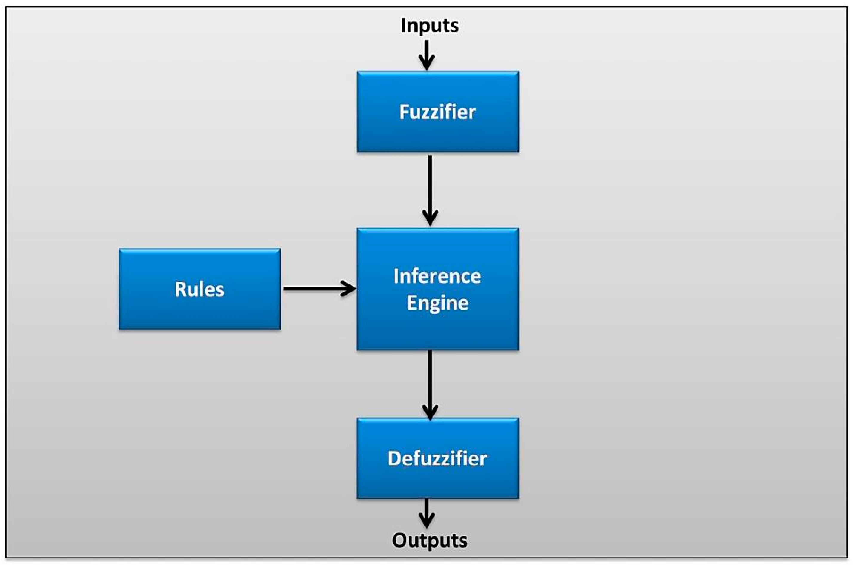
- The integration of sensor fusion using fuzzy logic rules based on sensor inputs and defined membership functions;
- -
- The capability of the mobile robot to follow a predetermined path;
- -
- The performance of the mobile robot when programmed with the fuzzy logic sets and rules.
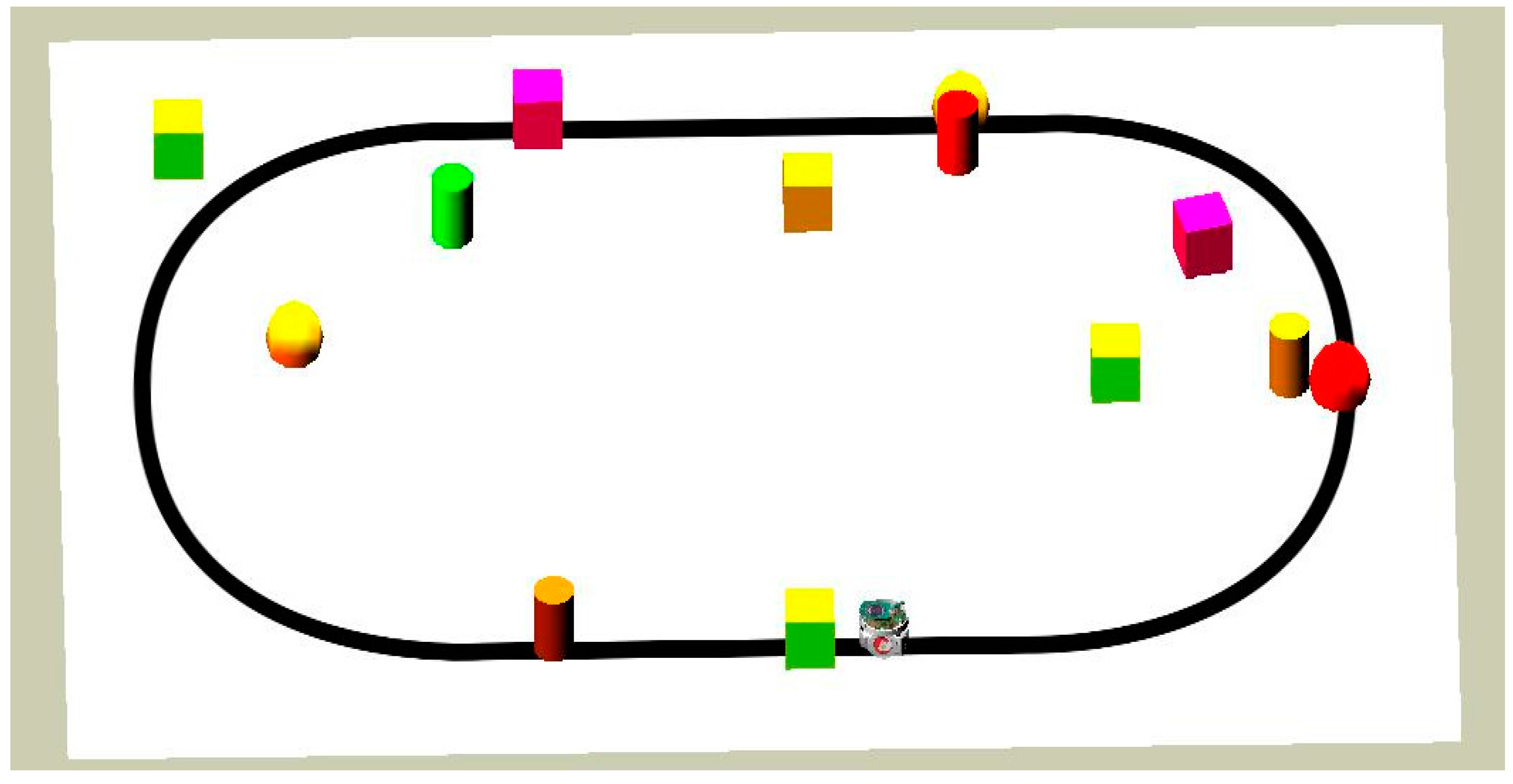
3.1. Robot and Environment Modeling

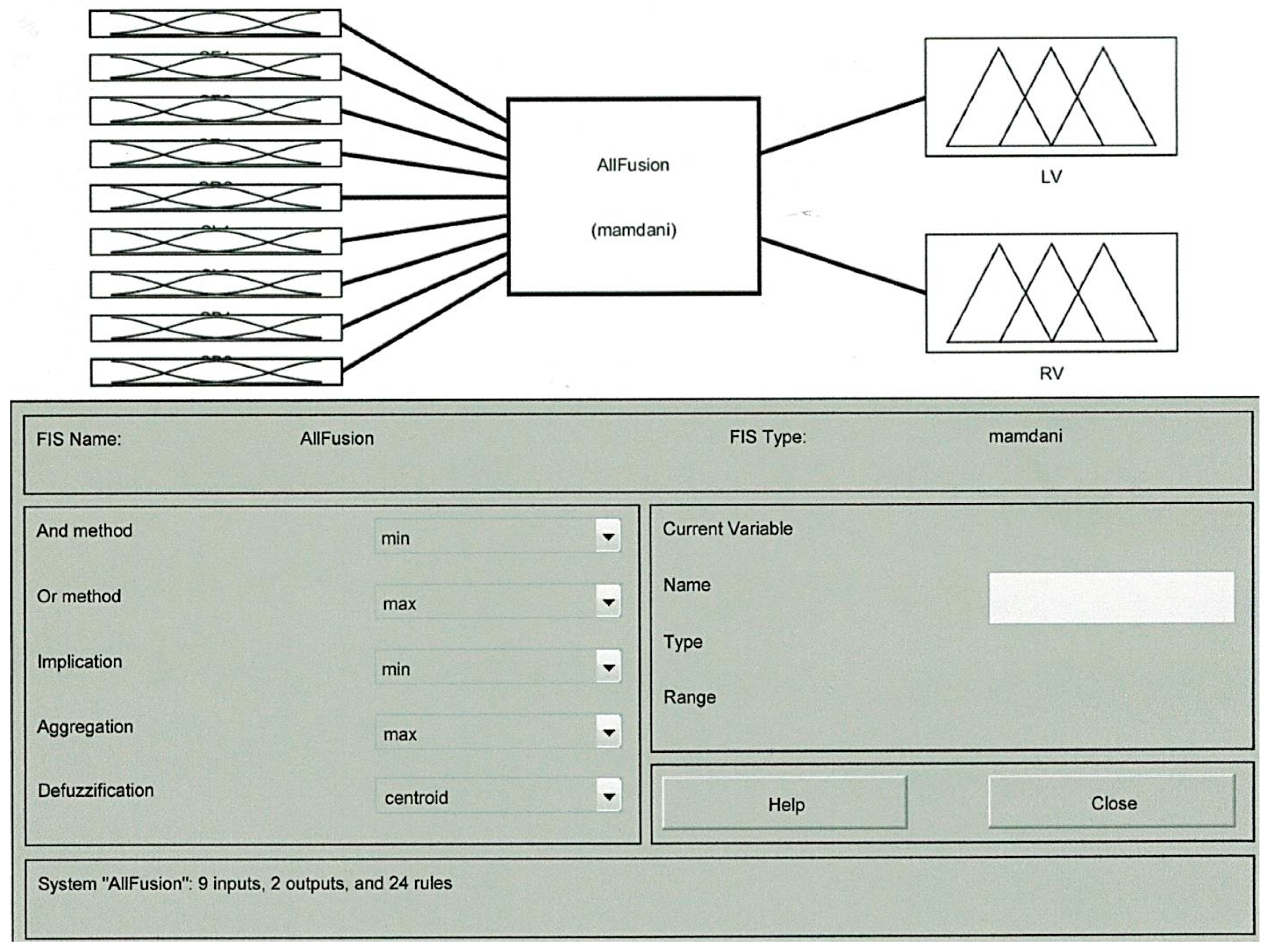
3.2. Design of the Fusion Model


3.2.1. Fuzzy Sets of the Input and Output
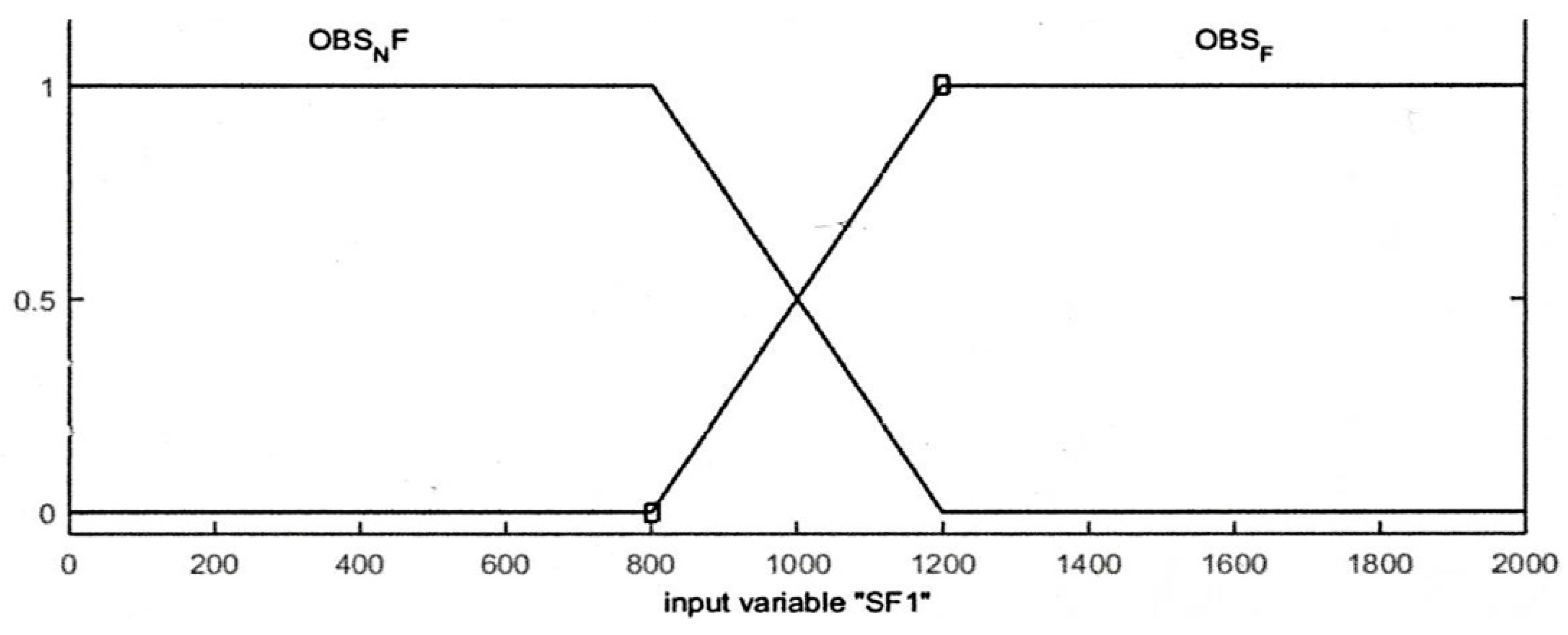
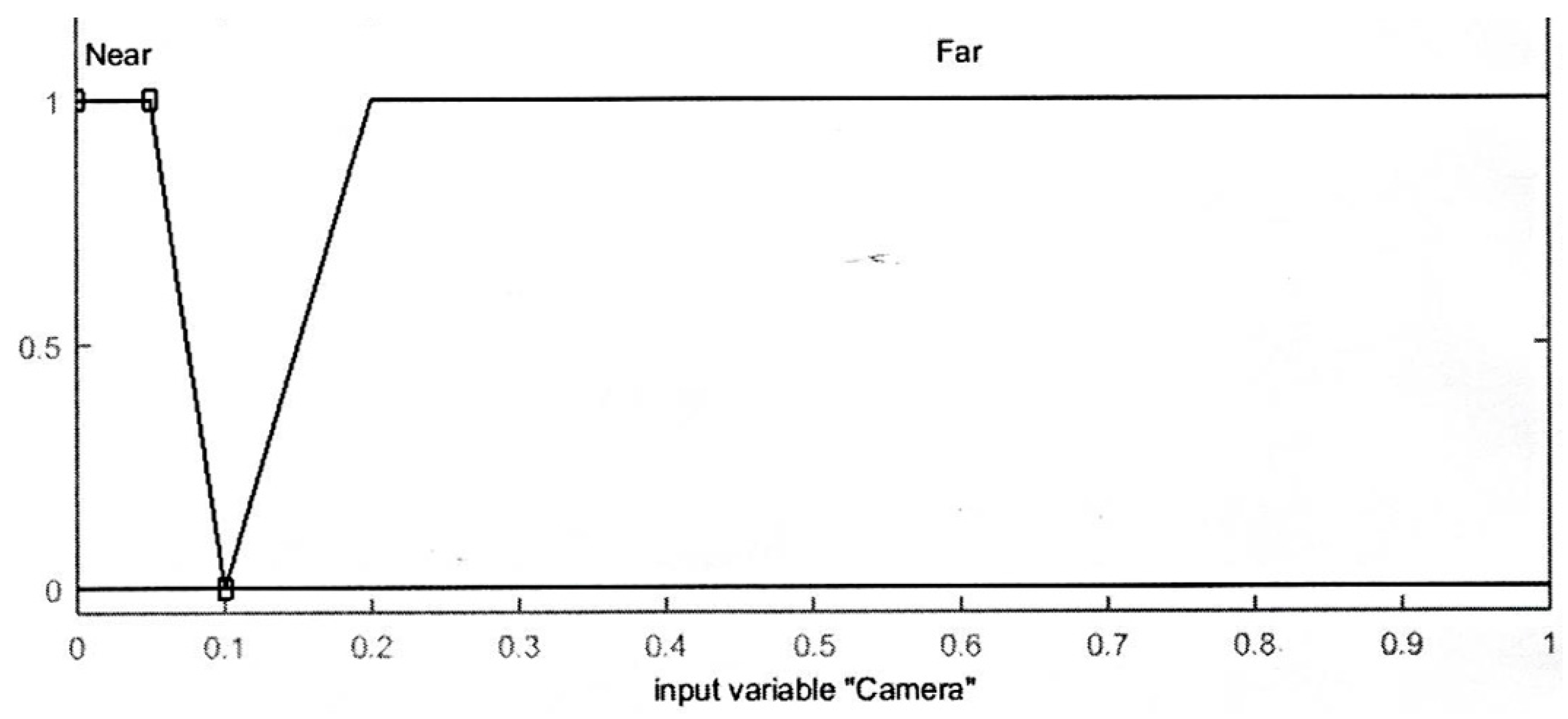
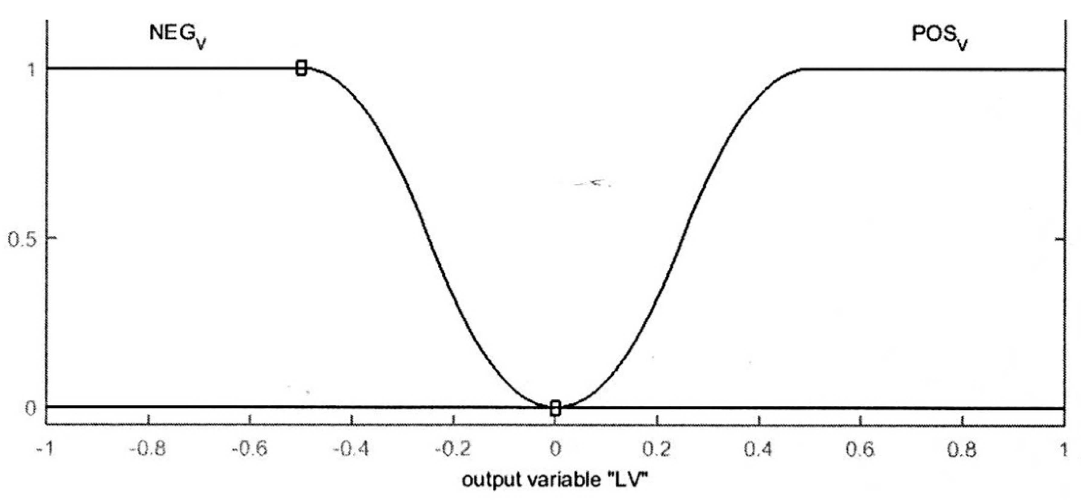
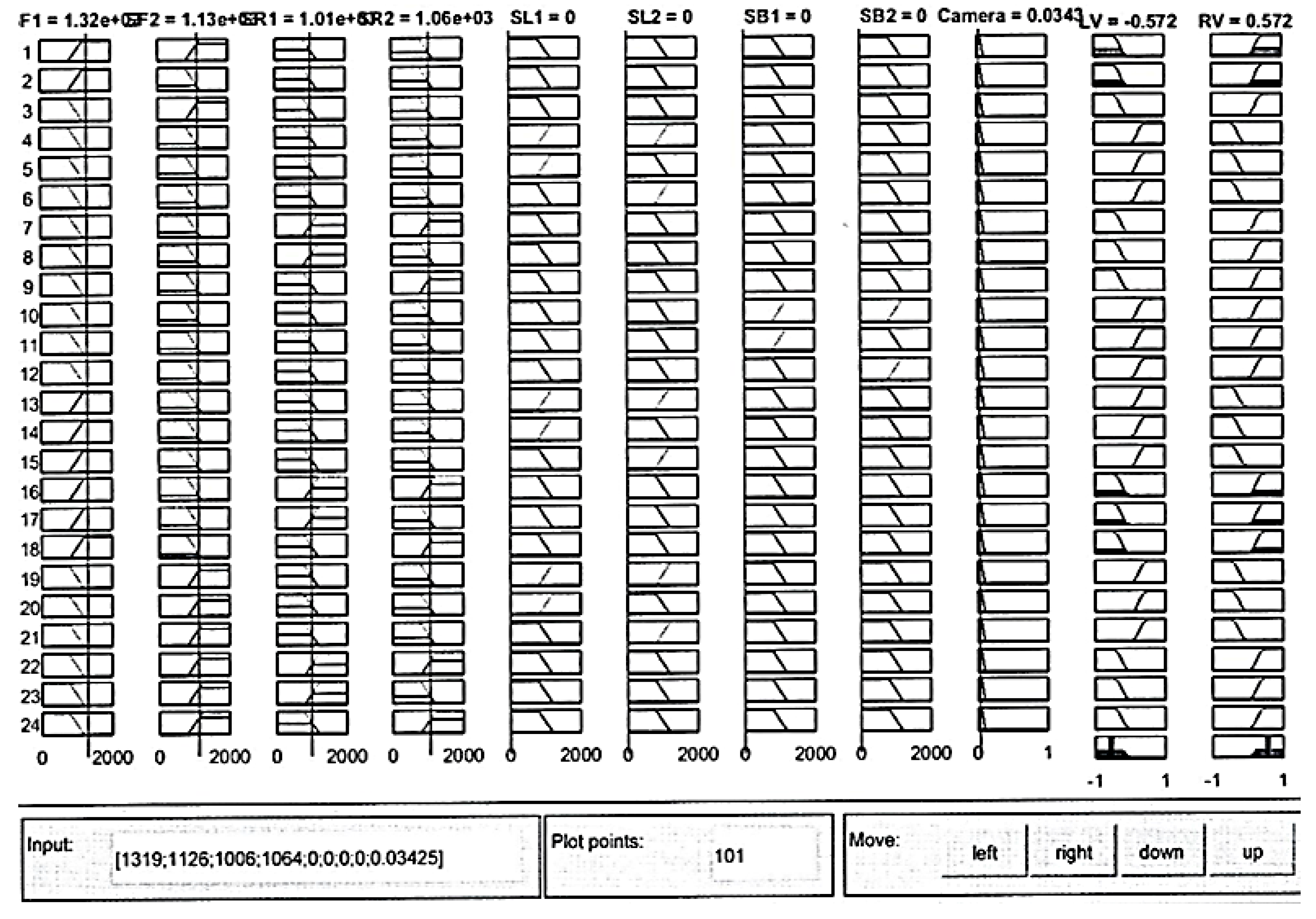
3.2.2. Membership Functions of the Input and Output
- -
- If both LV and RV speeds are set to POS_V, then the robot will move forward;
- -
- If LV is set to POS_V and RV is set to NEG_V, then the robot will turn right;
- -
- If LV is set to NEG_V and RV is set to POS_V, then the robot will turn left.


3.2.3. Designing Fuzzy Rules
3.2.4. Defuzzification

| No | SF1 | SF2 | SR1 | SR2 | SL1 | SL2 | SB1 | SB2 | LV | RV |
|---|---|---|---|---|---|---|---|---|---|---|
| 1 | OBS_F | OBS_F | OBS_NF | OBS_NF | OBS_NF | OBS_NF | OBS_NF | OBS_NF | NEG_V | POS_V |
| 2 | OBS_F | OBS_NF | OBS_NF | OBS_NF | OBS_NF | OBS_NF | OBS_NF | OBS_NF | NEG_V | POS_V |
| 3 | OBS_NF | OBS_F | OBS_NF | OBS_NF | OBS_NF | OBS_NF | OBS_NF | OBS_NF | NEG_V | POS_V |
| 4 | OBS_NF | OBS_NF | OBS_NF | OBS_NF | OBS_F | OBS_F | OBS_NF | OBS_NF | POS_V | NEG_V |
| 5 | OBS_NF | OBS_NF | OBS_NF | OBS_NF | OBS_F | OBS_NF | OBS_NF | OBS_NF | POS_V | NEG_V |
| 6 | OBS_NF | OBS_NF | OBS_NF | OBS_NF | OBS_NF | OBS_F | OBS_NF | OBS_NF | POS_V | NEG_V |
| 7 | OBS_NF | OBS_NF | OBS_F | OBS_F | OBS_NF | OBS_NF | OBS_NF | OBS_NF | NEG_V | POS_V |
| 8 | OBS_NF | OBS_NF | OBS_F | OBS_NF | OBS_NF | OBS_NF | OBS_NF | OBS_NF | NEG_V | POS_V |
| 9 | OBS_NF | OBS_NF | OBS_NF | OBS_F | OBS_NF | OBS_NF | OBS_NF | OBS_NF | NEG_V | POS_V |
| 10 | OBS_NF | OBS_NF | OBS_NF | OBS_NF | OBS_NF | OBS_NF | OBS_F | OBS_F | POS_V | POS_V |
| 11 | OBS_NF | OBS_NF | OBS_NF | OBS_NF | OBS_NF | OBS_NF | OBS_F | OBS_NF | POS_V | POS_V |
| 12 | OBS_NF | OBS_NF | OBS_NF | OBS_NF | OBS_NF | OBS_NF | OBS_NF | OBS_F | POS_V | POS_V |
| 13 | OBS_F | OBS_NF | OBS_NF | OBS_NF | OBS_F | OBS_F | OBS_NF | OBS_NF | POS_V | NEG_V |
| 14 | OBS_F | OBS_NF | OBS_NF | OBS_NF | OBS_F | OBS_NF | OBS_NF | OBS_NF | POS_V | NEG_V |
| 15 | OBS_F | OBS_NF | OBS_NF | OBS_NF | OBS_NF | OBS_F | OBS_NF | OBS_NF | POS_V | NEG_V |
| 16 | OBS_F | OBS_NF | OBS_F | OBS_F | OBS_NF | OBS_NF | OBS_NF | OBS_NF | NEG_V | POS_V |
| 17 | OBS_F | OBS_NF | OBS_F | OBS_NF | OBS_NF | OBS_NF | OBS_NF | OBS_NF | NEG_V | POS_V |
| 18 | OBS_F | OBS_NF | OBS_NF | OBS_F | OBS_NF | OBS_NF | OBS_NF | OBS_NF | NEG_V | POS_V |
| 19 | OBS_NF | OBS_F | OBS_NF | OBS_NF | OBS_F | OBS_F | OBS_NF | OBS_NF | POS_V | NEG_V |
| 20 | OBS_NF | OBS_F | OBS_NF | OBS_NF | OBS_F | OBS_NF | OBS_NF | OBS_NF | POS_V | NEG_V |
| 21 | OBS_NF | OBS_F | OBS_NF | OBS_NF | OBS_NF | OBS_F | OBS_NF | OBS_NF | POS_V | NEG_V |
| 22 | OBS_NF | OBS_F | OBS_F | OBS_F | OBS_NF | OBS_NF | OBS_NF | OBS_NF | NEG_V | POS_V |
| 23 | OBS_NF | OBS_F | OBS_F | OBS_NF | OBS_NF | OBS_NF | OBS_NF | OBS_NF | NEG_V | POS_V |
| 24 | OBS_NF | OBS_F | OBS_NF | OBS_F | OBS_NF | OBS_NF | OBS_NF | OBS_NF | NEG_V | POS_V |
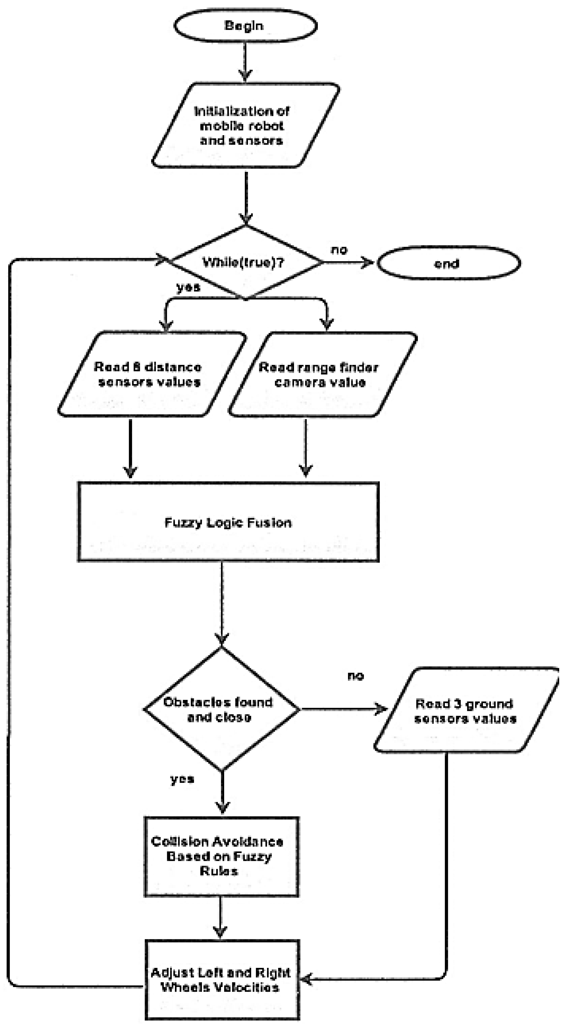
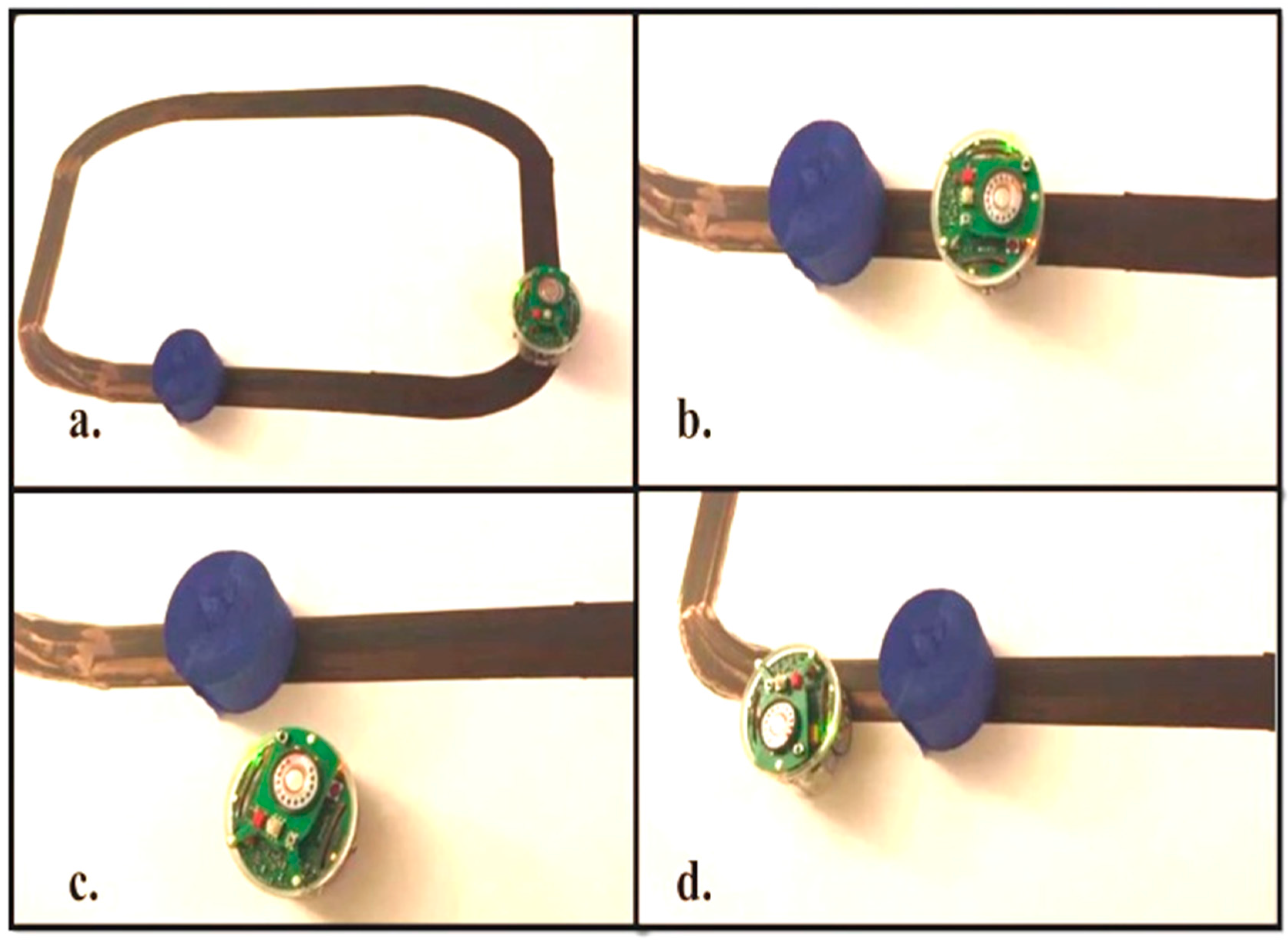
4. Simulation and Real Time Implementation for Mobile Robot Navigation


5. Results and Investigation of the Proposed Model
5.1. Data Collection and Analysis
5.1.1. First Scenario

| Distance Sensor | Without Fuzzy Logic Fusion | With Fuzzy Logic Fusion | ||||
|---|---|---|---|---|---|---|
| T1 = 5 | T2 = 15 | T3 = 41 | T1 = 5 | T2 = 22 | T3 = 41 | |
| SF1 | 14.71 | 1159.18 | 64.05 | 11.73 | 1127.19 | 72.72 |
| SF2 | 35.19 | 220.33 | 53.72 | 48.48 | 1077.76 | 54.80 |
| SR1 | 59.53 | 24.41 | 40.20 | 45.69 | 35.14 | 42.40 |
| SR2 | 31.55 | 26.77 | 4.68 | 31.54 | 28.00 | 28.47 |
| SL1 | 23.78 | 36.03 | 59.58 | 21.23 | 58.54 | 31.90 |
| SL2 | 59.49 | 18.59 | 33.88 | 13.40 | 38.10 | 72.51 |
| SB1 | 19.99 | 91.65 | 14.64 | 22.21 | 56.23 | 59.42 |
| SB2 | 46.62 | 13.29 | 5.08 | 66.13 | 30.13 | 47.91 |
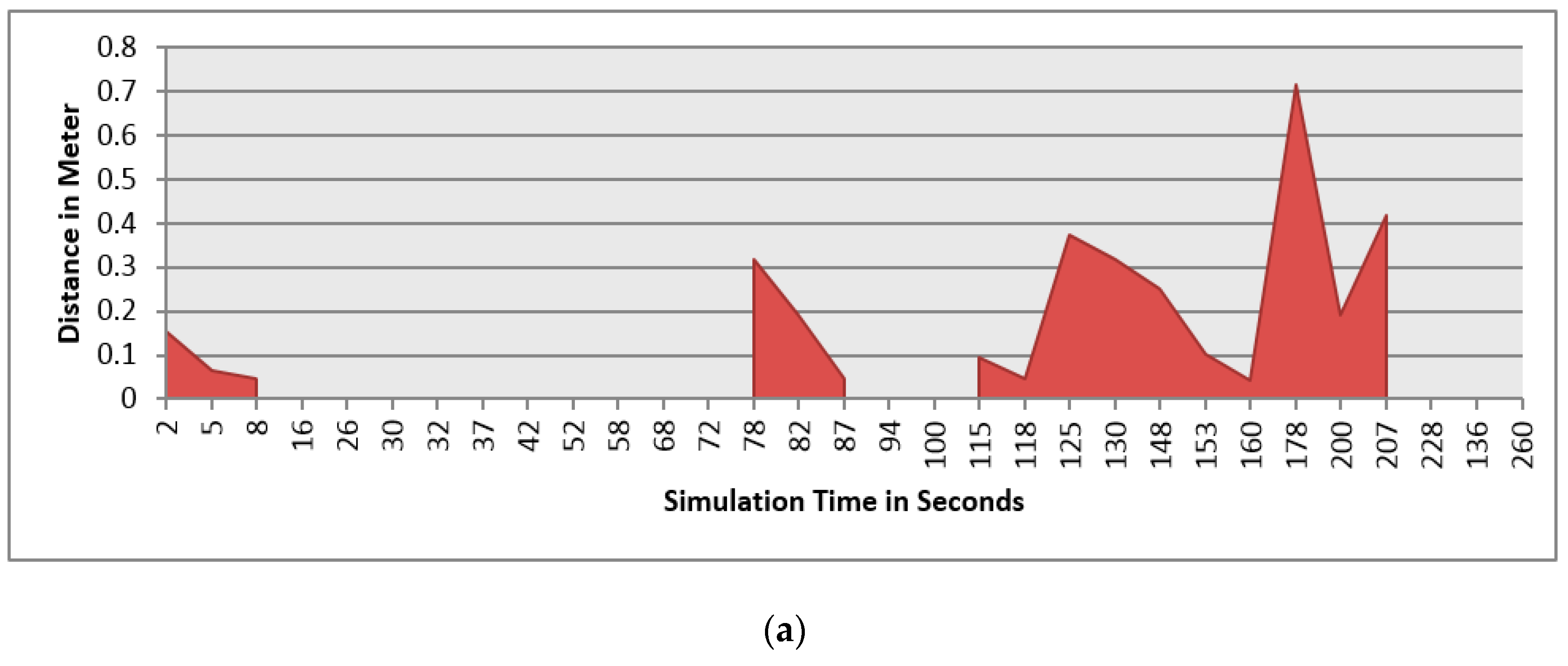
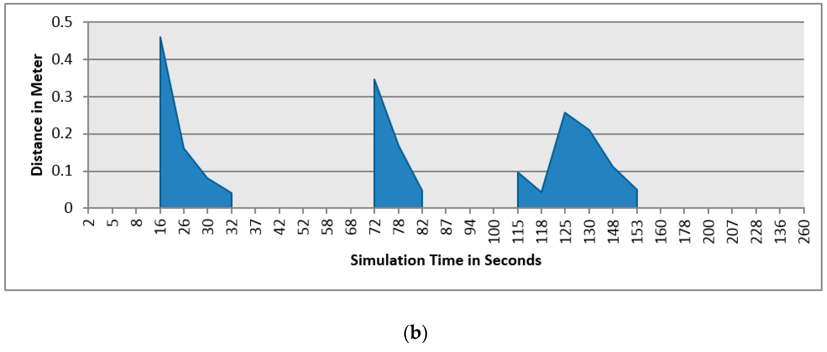
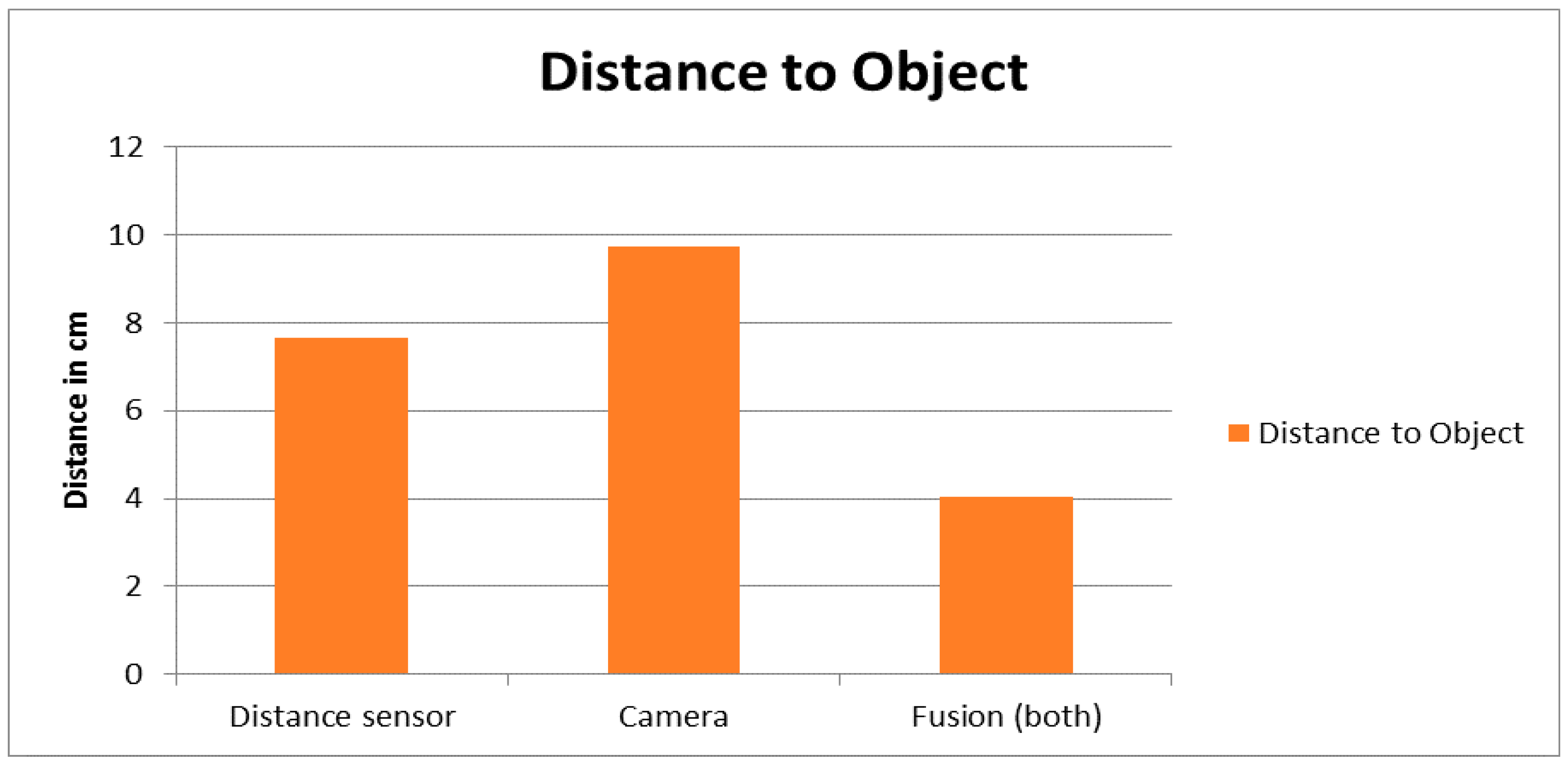
| Range Finder Camera | Without Fuzzy Logic Fusion | With Fuzzy Logic Fusion | ||||
|---|---|---|---|---|---|---|
| T1 = 5 | T2 = 13 | T3 = 41 | T1 = 5 | T2 = 22 | T3 = 41 | |
| Distance to Obstacle in Meter | 0.337 | 0.097 | x | 0.339 | 0.040 | x |
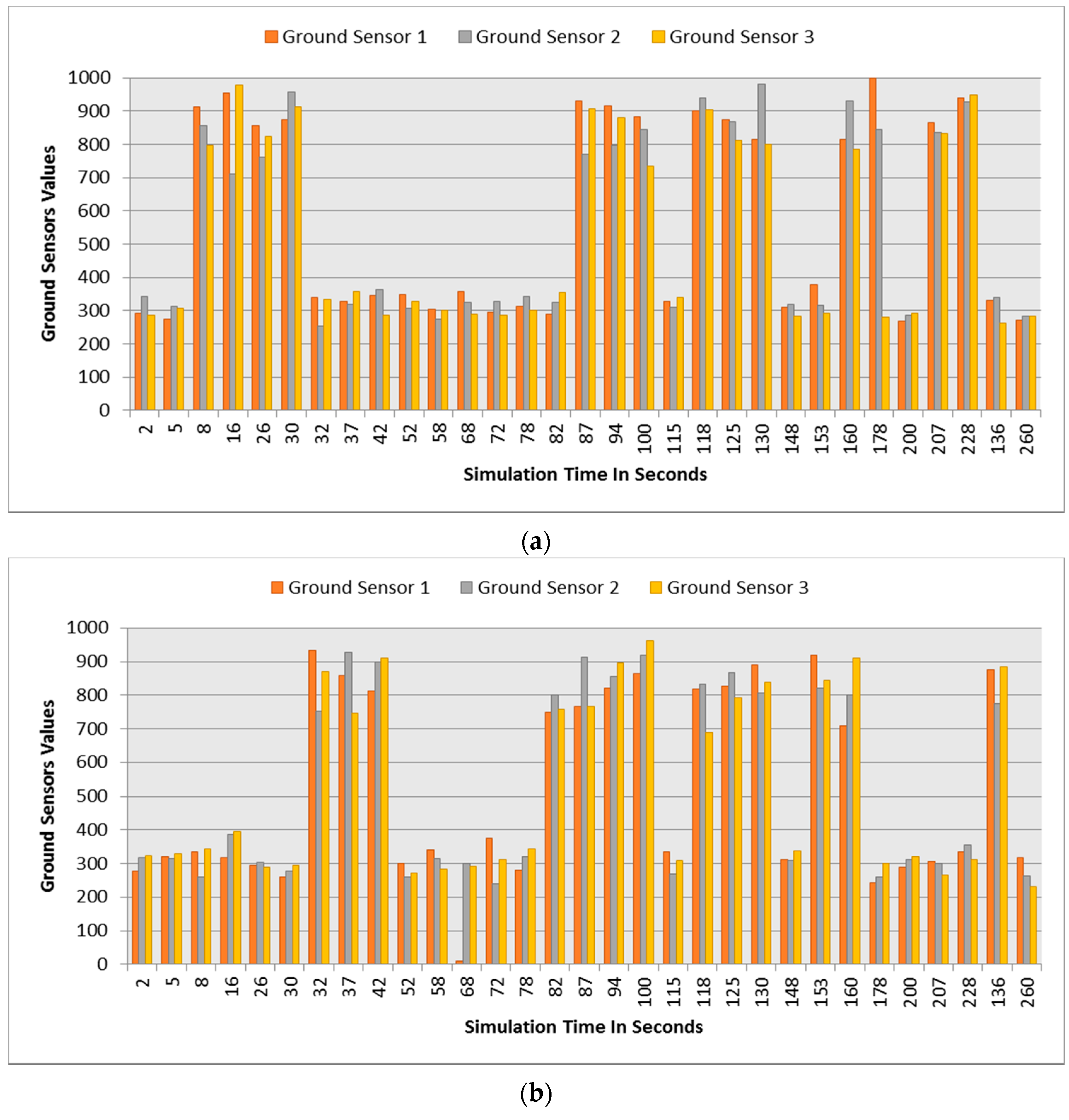
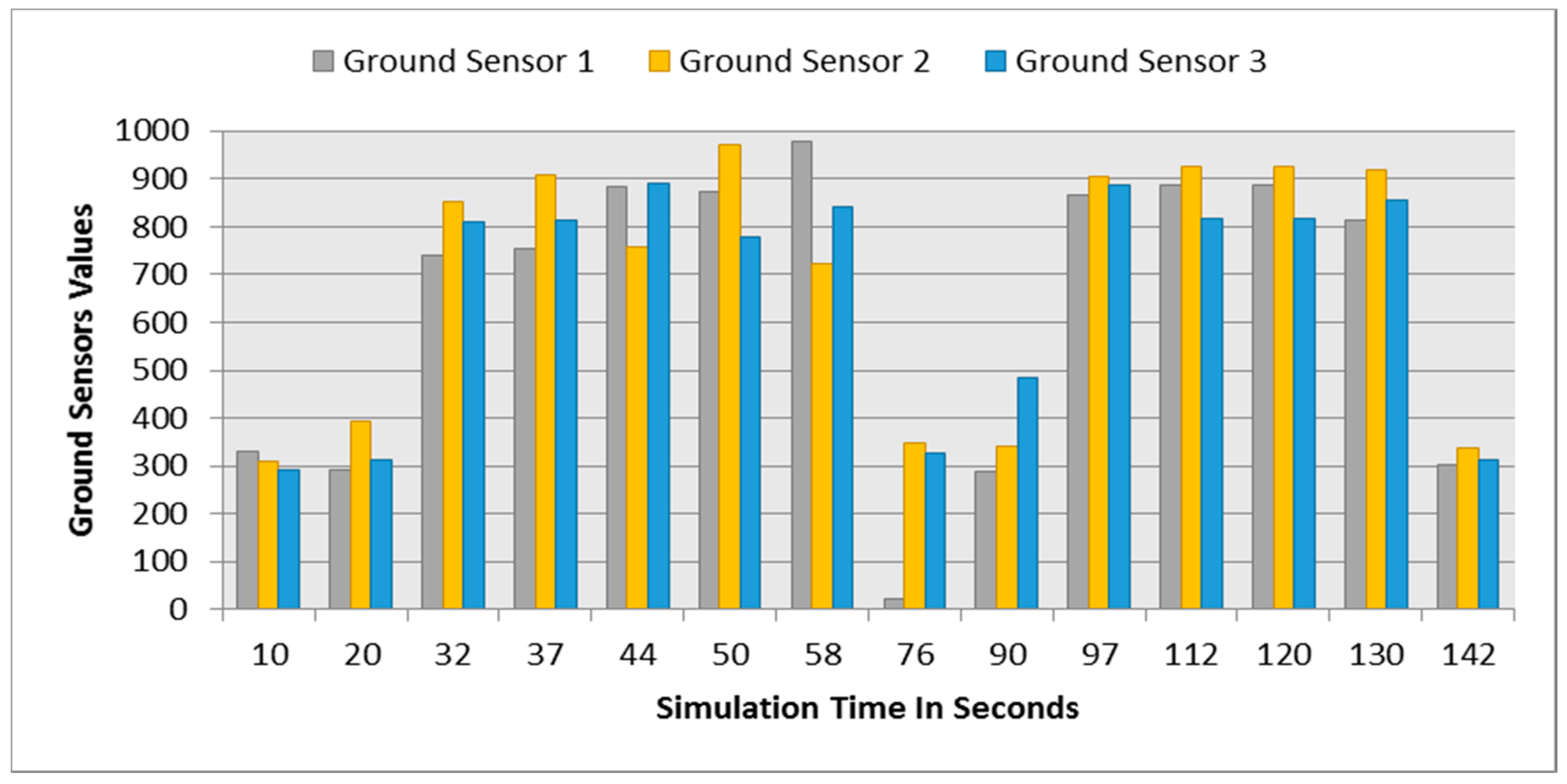
| Simulation Time | Ground Sensor 1 | Ground Sensor 2 | Ground Sensor 3 | Delta |
|---|---|---|---|---|
| 5 | 287.83 | 256.58 | 330.61 | 42.77 |
| 10 | 271.00 | 250.32 | 327.13 | 56.12 |
| 13 | 323.11 | 307.06 | 353.36 | 30.25 |
| 41 | 266.31 | 290.37 | 277.68 | 11.36 |
| Simulation Time in Seconds | Position | Rotation Angle in Degree θ | Left Wheel Velocity | Right Wheel Velocity | ||
|---|---|---|---|---|---|---|
| x | y | z | ||||
| 5 | 0.34 | 0.05 | 1.24 | −92.24 | 270.24 | 229.76 |
| 22 | 0.08 | 0.05 | 1.26 | −165.58 | −200.65 | 400.23 |
| 30 | 0.03 | 0.05 | 1.33 | −100.87 | 200.65 | 189.44 |
| 38 | −0.06 | 0.05 | 1.34 | −36.04 | 305.34 | −199.72 |
| 41 | −0.14 | 0.05 | 1.24 | −101.62 | 213.16 | 286.84 |
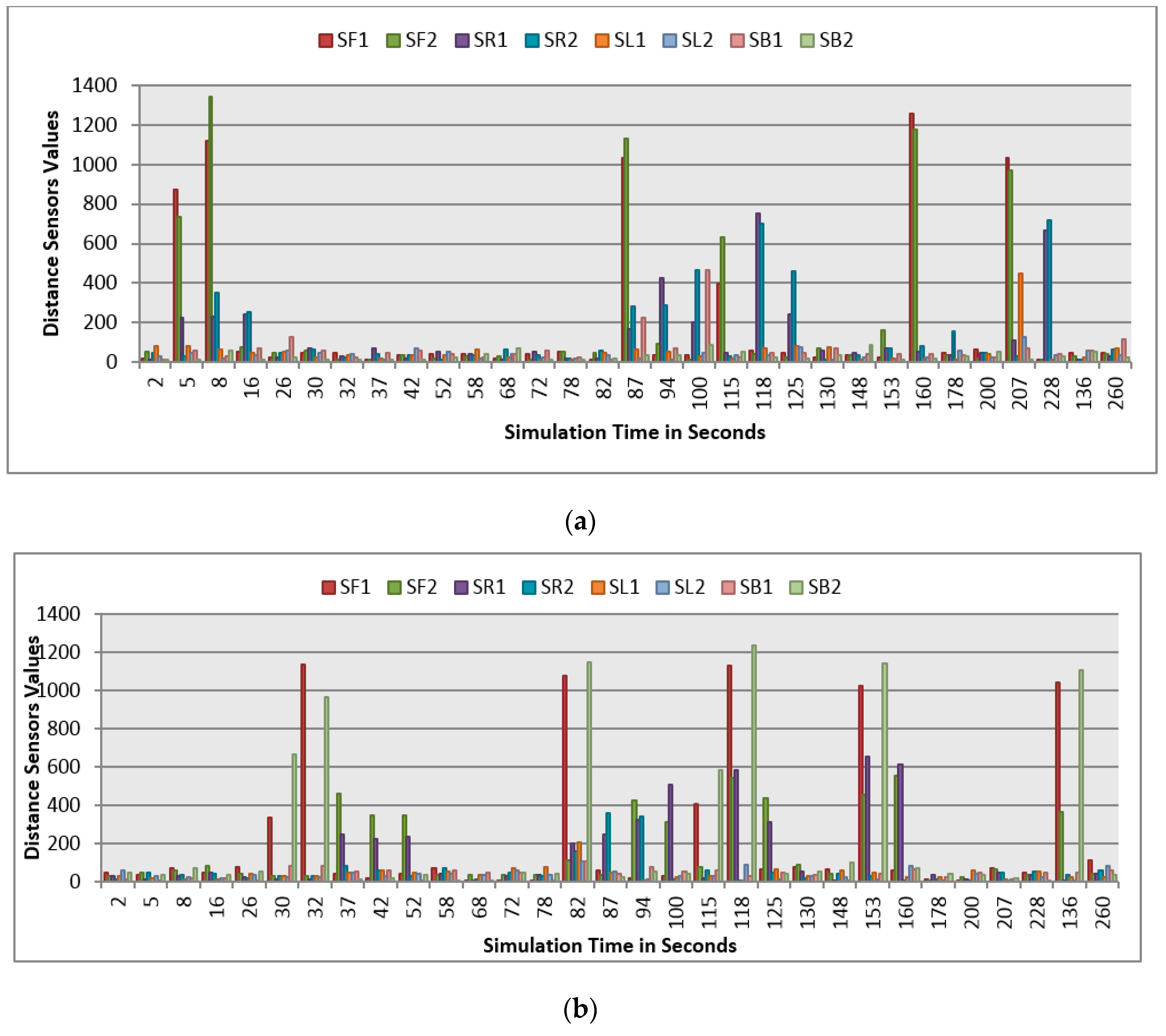
5.1.2. Second Scenario


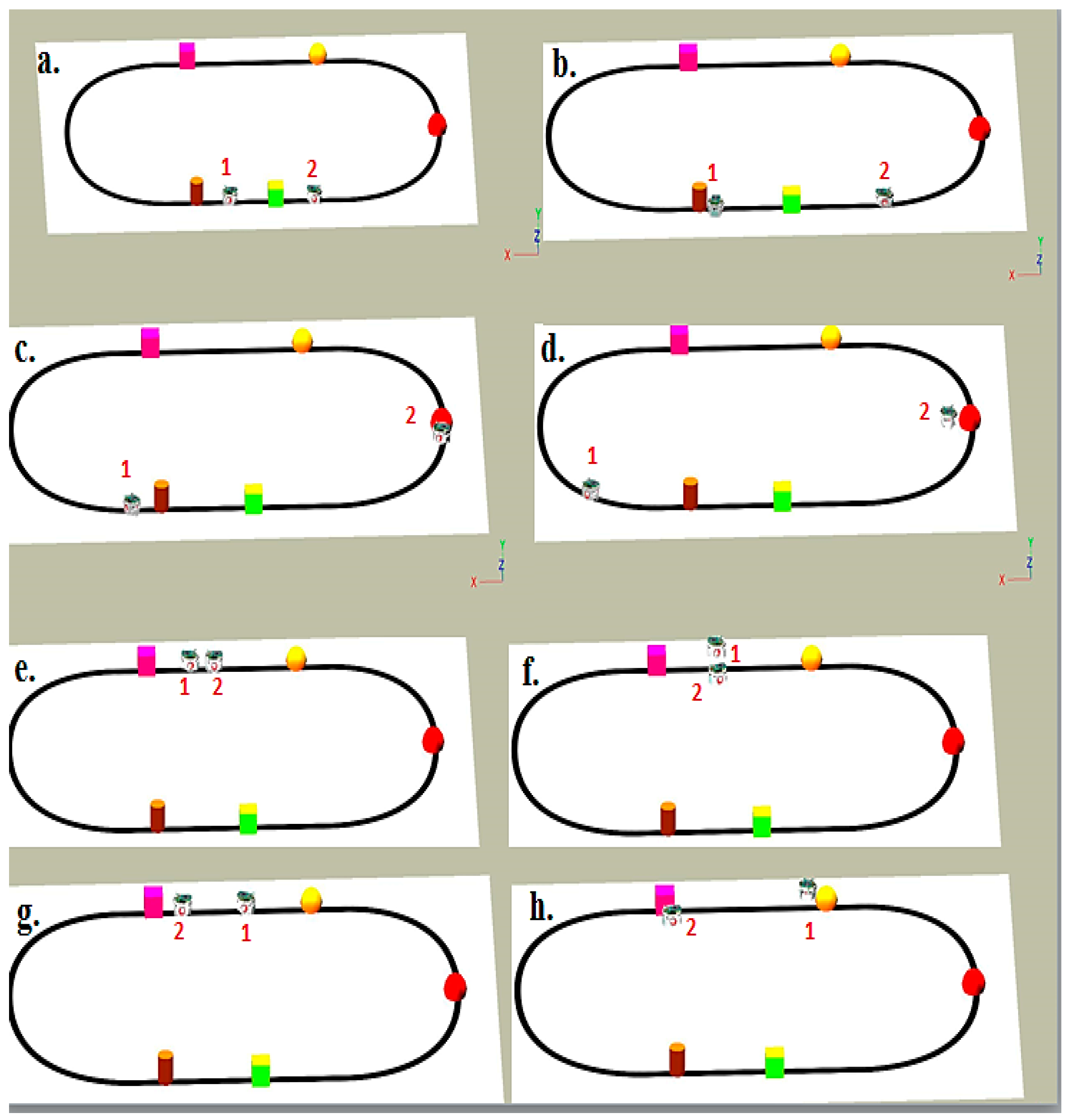
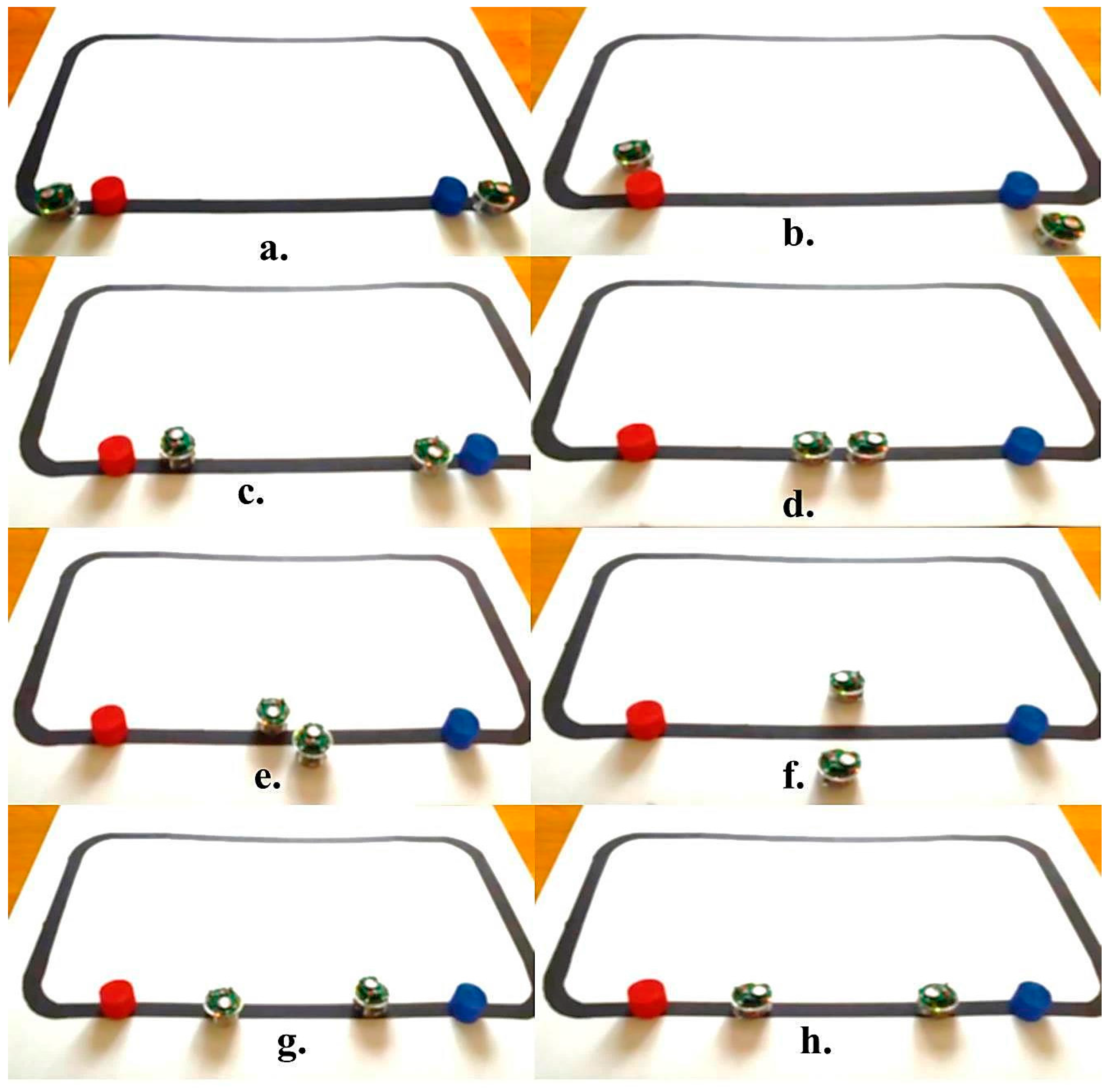
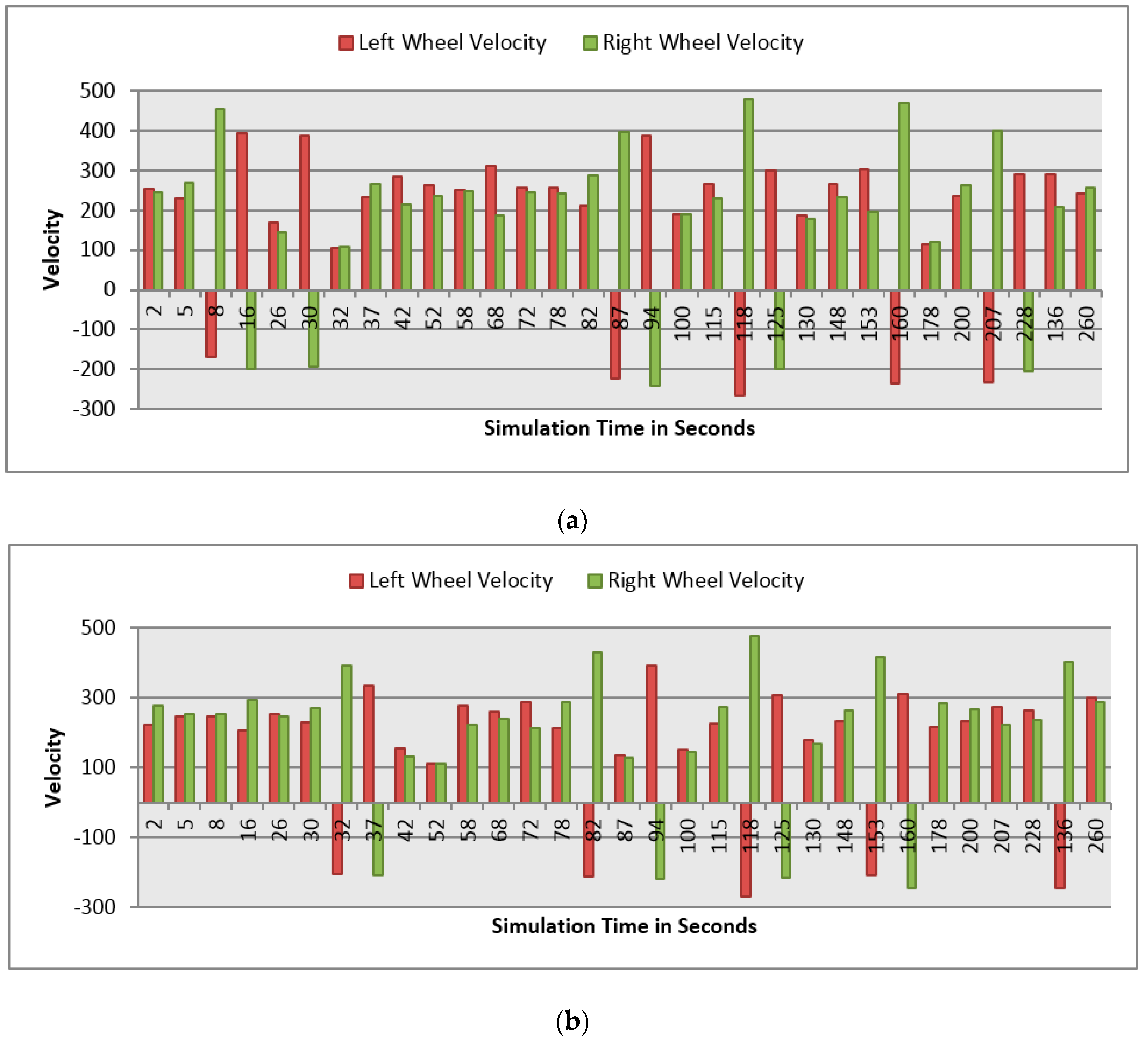
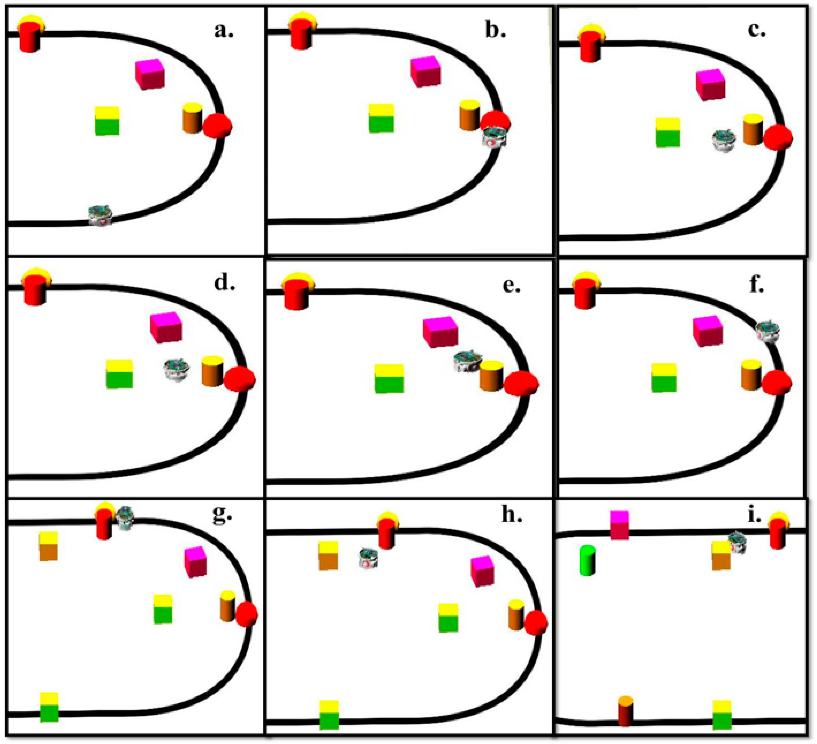
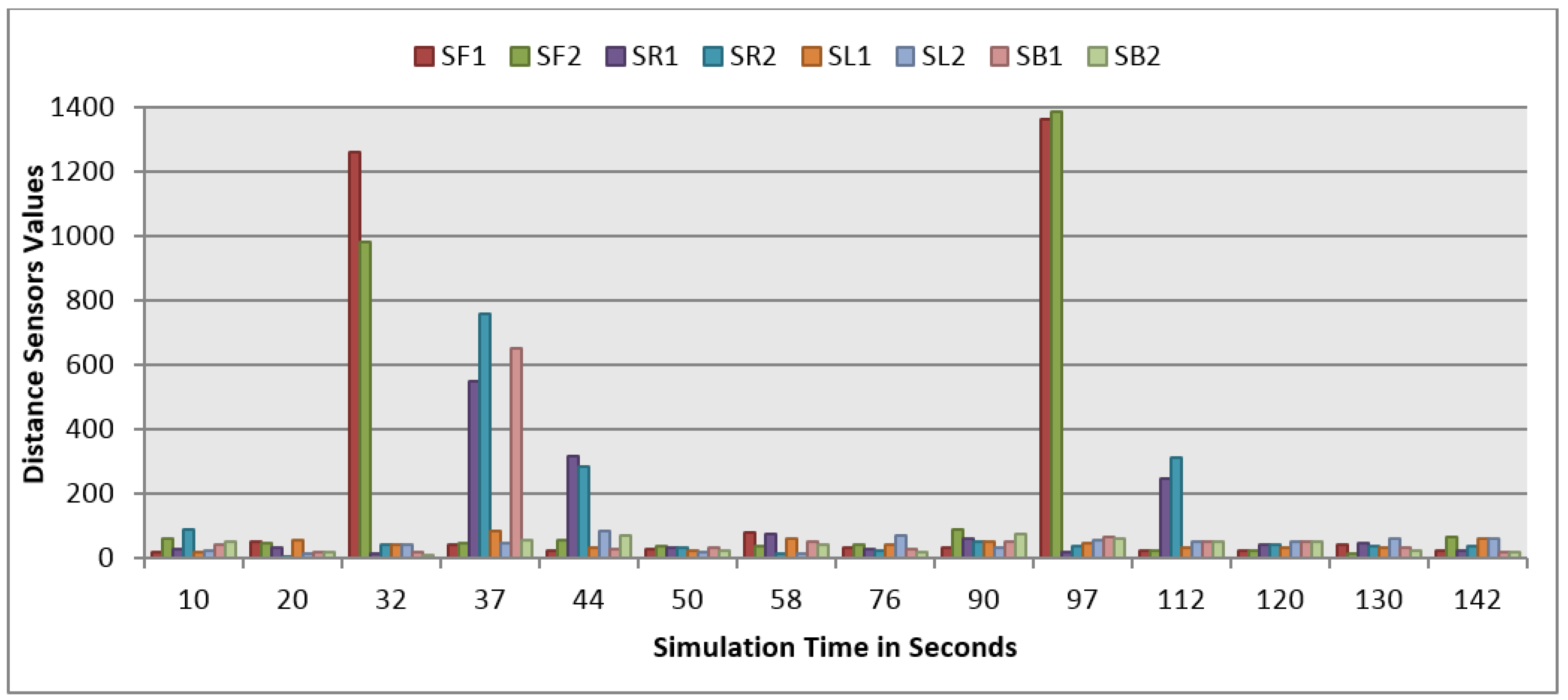
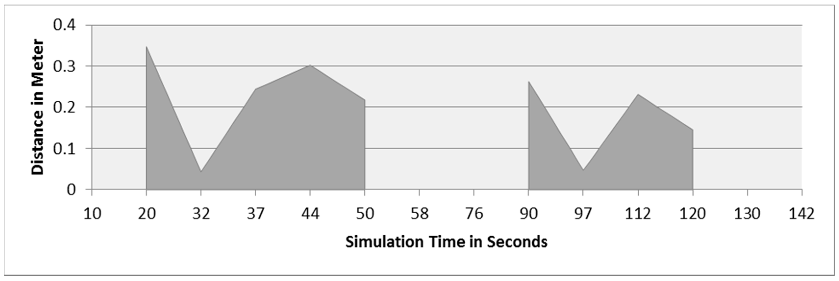
5.1.3. Third Scenario


| Simulation Time in Seconds | Robot 1 | Robot 2 | ||||||
|---|---|---|---|---|---|---|---|---|
| Position | Rotation Angle in Degree θ | Position | Rotation Angle in Degree θ | |||||
| x | y | z | x | y | z | |||
| 2 | 0.18 | 0.05 | 0.15 | 99.39 | −0.20 | 0.05 | 0.15 | −88.26 |
| 5 | 0.27 | 0.05 | 0.16 | 48.17 | −0.31 | 0.05 | 0.15 | −93.40 |
| 8 | 0.28 | 0.05 | 0.13 | 16.01 | −0.40 | 0.05 | 0.15 | −93.94 |
| 16 | 0.33 | 0.05 | 0.07 | 80.73 | −0.62 | 0.05 | 0.23 | −125.41 |
| 26 | 0.43 | 0.05 | 0.11 | 145.54 | −0.79 | 0.05 | 0.52 | −167.63 |
| 30 | 0.46 | 0.05 | 0.15 | 145.54 | −0.79 | 0.05 | 0.59 | 110.00 |
| 32 | 0.47 | 0.05 | 0.16 | 145.54 | −0.77 | 0.05 | 0.59 | 110.00 |
| 37 | 0.59 | 0.05 | 0.17 | 107.47 | −0.72 | 0.05 | 0.62 | 174.72 |
| 42 | 0.73 | 0.05 | 0.23 | 127.69 | −0.72 | 0.05 | 0.68 | 174.71 |
| 52 | 0.90 | 0.05 | 0.51 | 167.23 | −0.78 | 0.05 | 0.76 | −120.48 |
| 58 | 0.92 | 0.05 | 0.70 | 179.96 | −0.81 | 0.05 | 0.83 | 158.72 |
| 68 | 0.87 | 0.05 | 0.99 | −154.20 | −0.71 | 0.05 | 1.10 | 142.67 |
| 72 | 0.80 | 0.05 | 1.10 | −141.02 | −0.61 | 0.05 | 1.19 | 121.69 |
| 78 | 0.65 | 0.05 | 1.21 | −111.32 | −0.44 | 0.05 | 1.25 | 95.44 |
| 82 | 0.54 | 0.05 | 1.24 | −100.42 | −0.34 | 0.05 | 1.23 | 4.69 |
| 87 | 0.41 | 0.05 | 1.26 | −169.79 | −0.34 | 0.05 | 1.17 | 4.70 |
| 94 | 0.39 | 0.05 | 1.34 | −105.05 | −0.27 | 0.05 | 1.13 | 69.45 |
| 100 | 0.31 | 0.05 | 1.36 | −105.05 | −0.21 | 0.05 | 1.14 | 134.26 |
| 115 | 0.14 | 0.05 | 1.25 | 261.32 | 0.05 | 0.05 | 1.25 | 89.07 |
| 118 | 0.13 | 0.05 | 1.28 | −161.27 | 0.07 | 0.05 | 1.22 | 11.18 |
| 125 | 0.10 | 0.05 | 1.34 | −96.53 | 0.10 | 0.05 | 1.16 | 75.91 |
| 130 | 0.04 | 0.05 | 1.34 | −96.53 | 0.15 | 0.05 | 1.14 | 75.91 |
| 148 | −0.01 | 0.05 | 1.24 | 84.02 | 0.28 | 0.05 | 1.24 | 265.34 |
| 153 | −0.18 | 0.05 | 1.24 | −101.41 | 0.36 | 0.05 | 1.22 | 4.43 |
| 160 | −0.19 | 0.05 | 1.32 | −179.93 | 0.37 | 0.05 | 1.15 | 69.20 |
| 178 | −0.43 | 0.05 | 1.28 | −56.51 | 0.46 | 0.05 | 1.25 | 84.13 |
| 200 | −0.80 | 0.05 | 0.86 | −9.46 | 0.88 | 0.05 | 0.94 | 18.56 |
| 207 | −0.83 | 0.05 | 0.75 | −81.51 | 0.91 | 0.05 | 0.78 | 6.13 |
| 228 | −0.83 | 0.05 | 0.56 | 53.63 | 0.48 | 0.05 | 0.16 | −71.84 |
| 136 | −0.74 | 0.05 | 0.37 | 28.13 | 0.39 | 0.05 | 0.20 | −170.91 |
| 260 | −0.17 | 0.05 | 0.16 | 82.96 | 0.17 | 0.05 | 0.15 | −94.52 |


5.2. Results and Discussion


| Simulation Time in Seconds | Position | Rotation Angle in Degree θ | ||
|---|---|---|---|---|
| x | y | z | ||
| 10s | −0.46 | 0.05 | 0.16 | −101.09 |
| 20s | −0.72 | 0.05 | 0.33 | −147.02 |
| 32s | −0.79 | 0.05 | 0.59 | 109.58 |
| 37s | −0.71 | 0.05 | 0.62 | 109.58 |
| 44s | −0.65 | 0.05 | 0.65 | 174.30 |
| 50s | −0.64 | 0.05 | 0.74 | 175.88 |
| 58s | −0.68 | 0.05 | 0.80 | −119.31 |
| 76s | −0.78 | 0.05 | 0.93 | 171.94 |
| 90s | −0.52 | 0.05 | 1.23 | 107.53 |
| 97s | −0.34 | 0.05 | 1.23 | 9.67 |
| 112s | −0.27 | 0.05 | 1.07 | 74.42 |
| 120s | −0.19 | 0.05 | 1.05 | 92.64 |
| 130s | −0.11 | 0.05 | 1.14 | 139.23 |
| 142s | 0.05 | 0.05 | 1.24 | 81.03 |

6. Conclusions
Acknowledgments
Author Contributions
Conflicts of Interest
References
- Tian, J.; Gao, M.; Lu, E. Dynamic Collision Avoidance Path Planning for Mobile Robot Based on Multi-Sensor Data Fusion by Support Vector Machine. Mechatron. Autom. ICMA 2007, 2779–2783. [Google Scholar] [CrossRef]
- Hui, N.B.; Mahendar, V.; Pratihar, D.K. Time-optimal, collision-free navigation of a car-like mobile robot using neuro-fuzzy approaches. Fuzzy Sets Syst. 2006, 157, 2171–2204. [Google Scholar] [CrossRef]
- Al-Mayyahi, A.; Wang, W.; Birch, P. Adaptive Neuro-Fuzzy Technique for Autonomous Ground Vehicle Navigation. Robotics 2014, 3, 349–370. [Google Scholar] [CrossRef]
- Anjum, M.L.; Park, J.; Hwang, W.; Kwon, H.; Kim, J.; Lee, C.; Kim, K.; Cho, D. Sensor data fusion using Unscented Kalman Filter for accurate localization of mobile robots. In Proceedings of the 2010 International Conference on Control Automation and Systems (ICCAS), Gyeonggi-do, Korea, 27–30 October 2010; pp. 947–952.
- Nada, E.; Abd-Allah, M.; Tantawy, M.; Ahmed, A. Teleoperated Autonomous Vehicle. Int. J. Eng. Res. Technol. IJERT 2014, 3, 1088–1095. [Google Scholar]
- Chen, C.; Richardson, P. Mobile robot obstacle avoidance using short memory: A dynamic recurrent neuro-fuzzy approach. Trans. Inst. Measur. Control 2012, 34, 148–164. [Google Scholar] [CrossRef]
- Qu, D.; Hu, Y.; Zhang, Y. The Investigation of the Obstacle Avoidance for Mobile Robot Based on the Multi Sensor Information Fusion technology. Int. J. Mater. Mech. Manuf. 2013, 1, 366–370. [Google Scholar] [CrossRef]
- Kim, J.; Kim, J.; Kim, D. Development of an Efficient Obstacle Avoidance Compensation Algorithm Considering a Network Delay for a Network-Based Autonomous Mobile Robot. Inf. Sci. Appl. ICISA 2011, 1–9. [Google Scholar] [CrossRef]
- Rahul Sharma, K.; Honc, D.; Dusek, F. Sensor fusion for prediction of orientation and position from obstacle using multiple IR sensors an approach based on Kalman filter. Appl. Electron. AE 2014, 263–266. [Google Scholar] [CrossRef]
- Wang, J.; Liu, H.; Gao, M.; Sun, F.; Xiao, W. Information fusion-based mobile robot path control. Control Decis. Conf. CCDC 2012, 212–217. [Google Scholar] [CrossRef]
- Guo, M.; Liu, W.; Wang, Z. Robot Navigation Based on Multi-Sensor Data Fusion. Digit. Manuf. Autom. ICDMA 2011, 1063–1066. [Google Scholar] [CrossRef]
- Wang, Y.; Yang, Y.; Yuan, X.; Zuo, Y.; Zhou, Y.; Yin, F.; Tan, L. Autonomous mobile robot navigation system designed in dynamic environment based on transferable belief model. Measurement 2011, 44, 1389–1405. [Google Scholar]
- Wai, R.; Liu, C.; Lin, W. Design of switching path-planning control for obstacle avoidance of mobile robot. J. Frankl. Inst. 2011, 348, 718–737. [Google Scholar] [CrossRef]
- Canedo-Rodríguez, A.; Álvarez-Santos, V.; Regueiro, C.V.; Iglesias, R.; Barro, S.; Presedo, J. Particle filter robot localisation through robust fusion of laser, WiFi, compass, and a network of external cameras. Inf. Fusion 2016, 27, 170–188. [Google Scholar] [CrossRef]
- Chandrasenan, C.; Nafeesa, T.A.; Rajan, R.; Vijayakumar, K. Multisensor data fusion based autonomous mobile robot with manipulator for target detection. Int. J. Res. Eng. Technol. IJRET 2014, 3, 75–81. [Google Scholar]
- Cyberbotics.com, 2015. Available online: http://www.cyberbotics.com/overview (accessed on 23 December 2015).
© 2015 by the authors; licensee MDPI, Basel, Switzerland. This article is an open access article distributed under the terms and conditions of the Creative Commons by Attribution (CC-BY) license (http://creativecommons.org/licenses/by/4.0/).
Share and Cite
Almasri, M.; Elleithy, K.; Alajlan, A. Sensor Fusion Based Model for Collision Free Mobile Robot Navigation. Sensors 2016, 16, 24. https://doi.org/10.3390/s16010024
Almasri M, Elleithy K, Alajlan A. Sensor Fusion Based Model for Collision Free Mobile Robot Navigation. Sensors. 2016; 16(1):24. https://doi.org/10.3390/s16010024
Chicago/Turabian StyleAlmasri, Marwah, Khaled Elleithy, and Abrar Alajlan. 2016. "Sensor Fusion Based Model for Collision Free Mobile Robot Navigation" Sensors 16, no. 1: 24. https://doi.org/10.3390/s16010024