The Successive Projection Algorithm (SPA), an Algorithm with a Spatial Constraint for the Automatic Search of Endmembers in Hyperspectral Data

Abstract

Spectral mixing is a problem inherent to remote sensing data and results in few image pixel spectra representing ″pure″ targets. Linear spectral mixture analysis is designed to address this problem and it assumes that the pixel-to-pixel variability in a scene results from varying proportions of spectral endmembers. In this paper we present a different endmember-search algorithm called the Successive Projection Algorithm (SPA). SPA builds on convex geometry and orthogonal projection common to other endmember search algorithms by including a constraint on the spatial adjacency of endmember candidate pixels. Consequently it can reduce the susceptibility to outlier pixels and generates realistic endmembers.This is demonstrated using two case studies (AVIRIS Cuprite cube and Probe-1 imagery for Baffin Island) where image endmembers can be validated with ground truth data. The SPA algorithm extracts endmembers from hyperspectral data without having to reduce the data dimensionality. It uses the spectral angle (alike IEA) and the spatial adjacency of pixels in the image to constrain the selection of candidate pixels representing an endmember. We designed SPA based on the observation that many targets have spatial continuity (e.g. bedrock lithologies) in imagery and thus a spatial constraint would be beneficial in the endmember search. An additional product of the SPA is data describing the change of the simplex volume ratio between successive iterations during the endmember extraction. It illustrates the influence of a new endmember on the data structure, and provides information on the convergence of the algorithm. It can provide a general guideline to constrain the total number of endmembers in a search.

1. Introduction

Linear spectral mixture analysis (SMA) is based on the simple assumption that remotely sensed spectral measurements are mixed signatures that vary across the scene as the relative proportion of endmembers change. It is commonly used for the analysis of hyperspectral data [1-8], but to obtain accurate unmixing results the endmembers selected must be representative of surface components that occur in relatively pure form [9]. For this reason much literature has focused on the critical step of endmember extraction with the aim to determine the “purest” spectral representation of materials present in the scene.

Spectral endmembers can be derived from the imagery (image endmembers) or measurements in the laboratory/field (library endmembers). Library endmembers may not always be available, and if available, they are not necessarily acquired under the same conditions as airborne or satellite image data and may not be good representations of the image components. Thus there are advantages in being able to extract endmembers directly from imagery. The selection of image endmembers is typically achieved through the implicit (PPI, pixel purity index [10]) or explicit use of convex geometry [11]. A simplex is fit to the convex hull of the n-dimensional data cloud and the vertices of the simplex define the spectral properties of the endmembers. Based on this concept, a number of algorithms have been developed over the past decade to automatically find image endmembers and these include the N-FINDR [12], iterative error analysis (IEA) [13], vertex component analysis (VCA) [14], MaxD (Maximum Distance) [15], Sequential Maximum Angle Convex Cone (SMACC) [16], iterated constrained endmembers (ICE)[17], simplex growing algorithm (SGA) [18], minimum volume constrained nonnegative factorization (MVC-NMF) [19] and optical real-time adaptive spectral identification system (ORASIS) [20]. While these methods have proven effective under different situations, most use one pixel (the most extreme pixel) to represent one endmember, which results in the inclusion of outlier pixels (e.g. bad pixels) as endmembers. Indeed Howes et al. (2004) reported that convex-based endmember extraction methods were susceptible to outliers since only a single spurious pixel can significantly alter the endmember simplex [21]. Outliers may result for example from noise or atmospheric effects in the data.

In this paper we present a different endmember-search algorithm called the Successive Projection Algorithm (SPA). SPA builds on the convex geometry endmember search algorithms described above by including a constraint on the spatial adjacency of endmember candidate pixels, whereby this approach can reduce the susceptibility to outlier pixels and generates realistic endmembers. This is demonstrated using two case studies where image endmembers can be validated with ground truth data. The spatial constraint was introduced based on success we have had with the spatial-spectral endmember extraction algorithm (SSEE) that makes use of the spectral and spatial characteristics of image pixels during the search for image endmembers [22]. SSEE operates differently from SPA using a roving endmember search window that covers the entire input image and it was designed to find similar but distinct endmembers (e.g. spectrally similar but distinct rock units).

In Section 2, we present the concept of convex geometry and its relevance for endmember selection, followed by a summary of current convex-based endmember-search algorithms. In Section 3, we describe SPA and its functionality. Section 4 describes the characteristics of the two test datasets (AVIRIS Cuprite cube and Probe-1 imagery for Baffin Island) that are used to evaluate the SPA algorithm. The experimental results are presented in Section 5, followed by a discussion.

2. Background

2.1. Spectral endmembers in convex geometry

Linear spectral mixture analysis (LSMA) assumes that the pixel-to-pixel variability in a scene results from varying abundances of spectral endmembers. It follows that the spectral response for each pixel is a linear combination of endmember spectra, weighted by their fractional abundances. Assuming that the number of endmembers and their spectral signatures are known, the fractional abundances of endmembers in a given pixel are typically determined from a least squares fit [23, 24].

Let p⃗_(i,j) denote the spectrum for the pixel in the image coordinates (i, j), the foundation of LSMA can be defined by the following formulation

$${\overrightarrow{\mathit{\text{p}}}}_{(\mathit{\text{i}},\mathit{\text{j}})}=\sum _{\mathit{\text{k}}=1}^{\mathit{\text{m}}}{\mathit{\text{f}}}_{(\mathit{\text{i}},\mathit{\text{j}})\mathit{\text{k}}}{\overrightarrow{\mathit{\text{e}}}}_{\mathit{\text{k}}}+{\overrightarrow{\mathit{\text{ɛ}}}}_{(\mathit{\text{i}},\mathit{\text{j}})}$$

(1)

$${\mathit{\text{f}}}_{(\mathit{\text{i}},\mathit{\text{j}})\mathit{\text{k}}}\ge 0,\mathit{\text{k}}=1,\cdots ,\mathit{\text{m}},\sum _{\mathit{\text{k}}=1}^{\mathit{\text{m}}}{\mathit{\text{f}}}_{(\mathit{\text{i}},\mathit{\text{j}})\mathit{\text{k}}}=1$$

(2)

where m is the number of endmembers, e⃗_kis the kth endmember, ε⃗(_i,j) is the approximation error term (residual), which could be due to the noise in the data or due to modeling error (or both), and f_(i,j)k is the fractional abundance for the kth endmember of pixel (i, j).

Spectra can be represented as points in an n-dimensional scatter plot where n is the number of bands. If we omit the error term in (1), the possible linear mixtures computed from (1) and (2) form a simplex C_m defined by m vertices that are corresponding to the endmembers, e⃗₁,e⃗₂,⋯,e⃗_m [25]. According to Gritzmann and Klee (1994)[26], the volume of the simplex C_m can be calculated as

$$\mathit{\text{V}}(C_m)=\frac{1}{(\mathit{\text{m}}-1)!}{\left|det(\mathit{\text{W}}{W}^T)\right|}^{\frac{1}{2}}$$

(3)

where W =[e⃗₂ −e⃗₁,e⃗₃ −e⃗₁,⋯,e⃗_n −e⃗₁]. V(C_m) is the volume of the simplex defined by m endmembers, det(·) denotes the determinant of a matrix, |·| denotes the operation of absolute value. Once the endmembers (e⃗₁,e⃗₂,⋯,e⃗_m) are determined, their abundance can be estimated through the least squares method, which is equivalent to a projection on the simplex [25].

Using this framework, if all data points (pixels) are examined in n-dimensional space, endmembers present in the scene should be found at the vertices of the simplex. The interior space of the simplex then represents feasible mixtures. Thus, the task of finding endmembers is actually the identification of the simplex vertices, which has been the foundation for the geometric interpretation of hyperspectral data and for endmember extraction algorithms based on convex geometry. The spectral endmembers are determined as the spectral points closest to the vertices of the simplex formed by the image data in n-dimensional space, and are thus, the spectrally purest points of the image data.

The set of endmembers determined from convex geometry has the following properties that are relevant to the SPA algorithm proposed in this paper:

Property 1

The endmembers represent the pixels that contain the largest data “volume” [12, 26]. This property is used in the SPA algorithm to determine if it is converging.

Property 2

A vector (pixel) with maximum Euclidean norm (magnitude) must be located at one of the vertices of the simplex [25, 27]. It is the main step in SPA to identify pixels at the vertices of the simplex.

Property 3

For a given point in the simplex, a point with maximum distance must be a vertex of the simplex [27].

Property 4

The affine transformation (e.g. orthogonal projection) of a simplex is also a simplex, and endmembers are still located in the vertices of the new simplex after this transformation [14, 26]. In SPA this allows the use of orthogonal subspace projections as the core mechanism for endmember extraction.

2.2. Endmember extraction algorithms based on convex geometry

Search algorithms based on convex geometry rely on the four properties listed above, but differ in their approach to locate the vertices of the simplex. Such methods include PPI, N-FINDER, IEA, VCA, Max_D, ORASIS, SMACC, ICE, MVC-NMF and SGA. N-FINDER finds the set of pixels that define the simplex with the maximum volume inscribed within the dataset. IEA uses a series of constrained unmixing and chooses as the endmembers those pixels that minimize the residual error in the unmixing images. VCA and Max_D exploit the orthogonal projection approach to iteratively find the vertices of the simplex. SMACC is another algorithm for endmember extraction, which uses a convex cone model (also known as Residual Minimization) and constrained oblique projection to derive endmembers [16]. The patented ICE combines ideas from convex geometry and multivariate curve resolution techniques to find endmembers, which trades off goodness-of fit of the convex geometry model against the size of the simplex [17]. SGA finds a set of desired endmembers by growing a sequence of simplexes, improving the commonly used N-FINDR algorithm. ORASIS performs the endmember selection using the learning vector quantization (LVQ) concept and a minimum volume transform (MVT). MVC-NMF integrates the least squares analysis and the convex – geometry model by incorporating a volume constraint into the nonnegative matrix factorization (NMF). With the exception of ICE, ORASIS and MVC-NMF, the methods mentioned above have an assumption that vertices of the simplex (e.g. endmembers) can be represented by corresponding pixels in the scene. When no pixels in the scene match the vertices, the nearest pixels (e.g. mixtures) are selected. Whether this assumption is met is in part a function of the nature of the scene (spatial arrangement of targets) and the spatial resolution of the imagery. In the case of SMACC, N-FINDER, VCA, SGA and Max-D, one pixel (the most extreme pixel) is selected to represent one endmember and thus these methods suffer from the inherent sensitivity of convex geometry to outlier pixels [21]. Although principal component analysis (PCA), minimum noise fraction transform (MNF) and singular value decomposition (SVD) can be applied to the data prior to the endmember extraction to minimize the impact of noise [14, 28], these can also result in the loss of detection of useful endmember pixels characterized by subtle spectral detail. In order to overcome the outlier problem, IEA selects multiple pixels with a small spectral angle to the most extreme pixel, and the average of these pixels is used as an endmember. The robustness of this approach to noise is reported in Plaza's work on simulated data [29, 30]. However, in the case of isolated outlier pixels, the spectral angle between the outlier and other pixels can be large. In such a case IEA will still select the outlier pixel as an endmember resulting in a false endmember. An additional risk to the use of spectral angle for the selection of pixels that represent a given endmember is that these pixels may represent spatially distinct targets in the scene that are characterized by a similar spectral shape but with distinct subtle spectral difference as indicated by Turner II et al. (2004)[31]. In such a case the distinct character of each target would be lost due to spectral averaging and the lack of consideration of their spatial association. Thus one endmember would be identified rather then two.

3. The successive projection algorithm (SPA)

3.1. Spectral similarity and spatial adjacency as selection criteria

In this study we propose a more robust approach that uses the spectral angle (alike IEA) and the spatial adjacency of pixels in the image to constrain the selection of candidate pixels representing an endmember. Two assumptions are made: 1) pixels that are spatially adjacent are more likely to have similar spectral properties and thus represent one endmember, and, 2) the probability that two adjacent pixels are both spurious is low. These assumptions are certainly reasonable if the target application is geological mapping because mappable units (e.g. bedrock lithologies) typically have spectral properties with spatial continuity in hyperspectral imagery.

The next section (e.g. 3.2.) describes how a vertex (e.g. an extreme pixel) is identified based on its spectral uniqueness in the simplex (the distinctness is measured in terms of the vector Euclidean norm or the distance of the pixel to the subspace defined by the previously selected endmembers). A meaningful endmember for this vertex is then the average of multiple candidate pixels that are spectrally distinct (e.g. they are located at or near one of the corners of the simplex) and are spatially adjacent. To find these candidate pixels we construct a pixel set, P_possible, consisting of r pixels (the value of r is user defined and here set to 10) that are closest to the vertex (this step is identical to IEA).

Then a subset,

$${\mathit{\text{P}}}_{\mathit{\text{candidate}}}=\left\{{\overrightarrow{\mathit{\text{p}}}}_{({\mathit{\text{x}}}_1,{\mathit{\text{y}}}_1)},{\overrightarrow{\mathit{\text{p}}}}_{({\mathit{\text{x}}}_2,{\mathit{\text{y}}}_2)},\cdots ,{\overrightarrow{\mathit{\text{p}}}}_{(x_c,y_c)}\right\}(\mathit{\text{c}}\le \mathit{\text{r}},{\mathit{\text{P}}}_{\mathit{\text{candidate}}}\in {\mathit{\text{P}}}_{\mathit{\text{candidate}}}),$$

(4)

is selected from these r pixels (P_possible) subject to conditions ((5) and (6)):

$$x_i-x_j\le \mathit{\text{t}}\_\mathit{\text{pixel}}\mathbf{\text{AND}}{y}_i-y_j\le \mathit{\text{t}}\_\mathit{\text{pixel}}(\mathit{\text{i}}\ne \mathit{\text{j}}),$$

(5)

$$\mathit{\text{s}}\_\mathit{\text{angle}}({\overrightarrow{\mathit{\text{p}}}}_{(x_i,y_i)},{\overrightarrow{\mathit{\text{p}}}}_{(x_j,y_j)})\le \mathit{\text{t}}\_\mathit{\text{θ}}(\mathit{\text{i}}\ne \mathit{\text{j}})$$

(6)

where x_i,y_i are pixel image coordinates, and t _pixel is a threshold value in pixels defining the acceptable spatially adjacency. The smallest possible value is 1 pixel to avoid the inclusion of mixed pixels. If the scene is not spatially complex, this value can be increased. The s_angle(p⃗_xi,yi;,p⃗_(xj,yj)) is the spectral angle between two spectra and is calculated as

$$\mathit{\text{s}}\_\mathit{\text{angle}}({\overrightarrow{\mathit{\text{p}}}}_{(x_i,y_i)},{\overrightarrow{\mathit{\text{p}}}}_{(x_j,y_j)})={cos}^{-1}\left(\frac{{\overrightarrow{\mathit{\text{p}}}}_{(x_i,y_i)}•{\overrightarrow{\mathit{\text{p}}}}_{(x_j,y_j)}}{\left|{\overrightarrow{\mathit{\text{p}}}}_{(x_i,y_i)}\right|\left|{\overrightarrow{\mathit{\text{p}}}}_{(x_j,y_j)}\right|}\right),$$

(7)

and t _θ is the threshold value for the spectral angle beyond which two spectra are not considered similar. The value of t _θ was set at 2.5 degrees based on experiments.

The average vector of P_candidate, represents one endmember spectrum. When no pixels in P_possible satisfy the conditions (5) and (6), the most extreme pixel in P_possible is selected as the endmember.

3.2. Description of the SPA algorithm

SPA starts by identifying the two most distinct endmembers, e⃗₁and e⃗₂, typically representing respectively the brightest and darkest pixels. It then iteratively finds remaining endmembers, using orthogonal projections, until the number of endmembers defined by the user is obtained. Below is a step-by-step description of the SPA algorithm.

Step 1: Parameter setting

Values for the following three parameters must be set: the number of endmembers(m) to find, the spectral angle threshold (t _θ) and the spatial threshold (t _pixel).

Step 2: Extraction of the first endmember (e⃗₁)

The vector norms of all pixels in the image are calculated to locate the pixel that has the largest norm. According to Property 2, this pixel is at one of the simplex vertices and typically is the brightest pixels in the image cube. The first endmember e⃗₁ is then estimated as described in Section 3.1.

Step 3: Extraction of the second endmember (e⃗₂)

The distances between all pixels and e⃗₁ are calculated and the pixel that has the largest distance is located. According to Property 3, this pixel will be at another vertex of the simplex usually corresponding to the darkest object in the scene (e.g. water body or shade). The 2^nd endmember, e⃗₂, can then be estimated according to section 3.1.

Step 4: Orthogonal projection and extraction of a new endmember

An endmember matrix U =[e⃗₁, e⃗₂] is then constructed using the two previously defined endmembers, and all pixels are projected to the subspace, S_proj, orthogonal to the space spanned by U as

$${\overrightarrow{\mathit{\text{p}}}}_{(\mathit{\text{i}},\mathit{\text{j}})\_\mathit{\text{proj}}}=\mathit{\text{O}}{\overrightarrow{\mathit{\text{p}}}}_{(\mathit{\text{i}},\mathit{\text{j}})},$$

(8)

where p⃗_(i,j)__{proj and p⃗(i,j)} are the projected and original pixel vector at image location (i, j) respectively. O is the projection operator,

$$\mathit{\text{O}}=\mathit{\text{I}}-\mathit{\text{U}}{\mathit{\text{U}}}^{+},$$

(9)

where I is the identity matrix, and U⁺ is the pseudo inverse of U, denoted by

$${\mathit{\text{U}}}^{+}={(U^T\mathit{\text{U}})}^{-1}{U}^T.$$

(10)

In the projected subspace (S_proj), the contribution to the mixtures from endmembers in U is eliminated. According to Property 4, the projected data in the new space still conform to the convexity, that is to say the endmembers are still at the vertices of the simplex. The vector (pixel) with the maximum norm in the projected subspace (S_proj) will correspond to a new endmember (Property 2) in this case e⃗₃, and this pixel is located at the apex of the simplex furthest away from the subspace spanned by the previously defined endmembers, e⃗₁ and e⃗₂.

Step 5: Complete the search of all endmembers

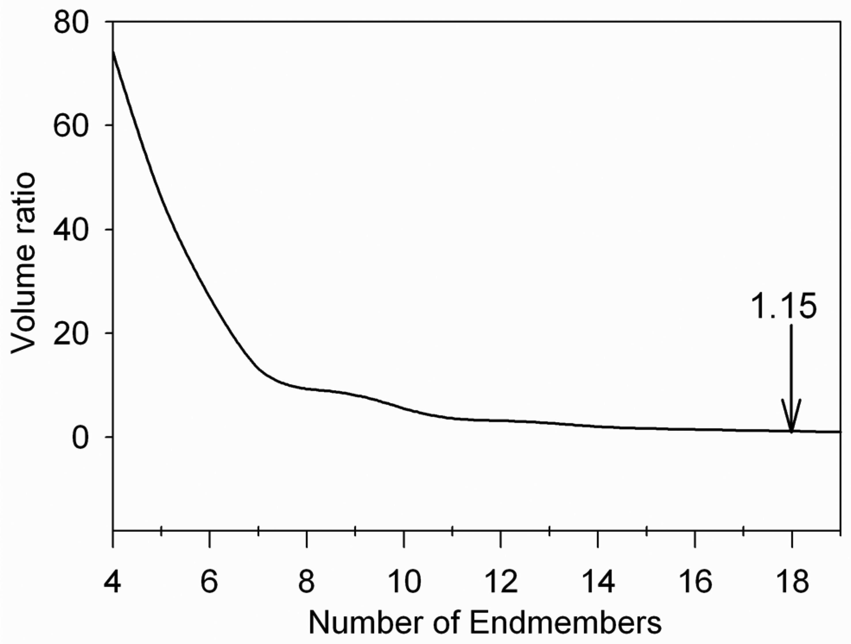
The endmember matrix, U = [e⃗₁, e⃗₂, e⃗₃], is then updated and Step 4 repeated to define a new endmember. This step is repeated until the predetermined number (m) of endmembers is reached.

We calculate the change of the simplex volume with each subspace projection because it provides an insight on the convergence of the algorithm. The volume of the simplex can be calculated only when the simplex has more than 3 vertices. According to Property 1, the complete endmember set defines a simplex with the maximum volume, assuming that a simplex can fit the hyperspectral data perfectly. Thus, as a new endmember is estimated from the data, a new vertex is added to the simplex defined by the previous endmembers, and the volume of the simplex increases until the requested number of endmembers is reached. The volume increase is determined by the spectral contrast between the current endmember and the previously defined endmember set. Assuming data with m endmembers, if C_l–1 and Cl denote the simplexes defined by the current endmember set, {e⃗₁,e⃗₂, ⋯, e⃗_l-1, e⃗_l} and the previous endmember set {e⃗₁,e⃗₂, ⋯,e⃗_l-1}, the ratio of the volumes of Cl and C_l–1 can be calculated as

$$\mathit{\text{ν}}\_{\mathit{\text{ratio}}}_l=\frac{\mathit{\text{V}}(C_l)}{\mathit{\text{V}}({\mathit{\text{C}}}_{\mathit{\text{l}}-1})},(3<\mathit{\text{l}}\le \mathit{\text{m}}).$$

(11)

As endmembers are selected (e.g. the value of l is approaching m), the ν_ratio_l decreases and theoretically converges to 1.0 if the simplex can fit the hyperspectral data very well [32]. The noise level and the complexity of the data will impact how quickly the volume ratio (ν_ratio_l) converges and whether it converges to 1.0.

4. Description of the test data

The SPA algorithm was evaluated using two hyperspectral datasets. The first one was collected over the Cuprite mining district, Nevada, in July 1995 wit the Airborne Visible Infra-Red Imaging Spectrometer (AVIRIS) as part of an AVIRIS Group Shoot [2] and is available in the tutorial CD of the ENVI software. The second dataset was acquired by the Probe-1 airborne hyperspectral sensor flown over Baffin Island, Canada in July 2000. Before describing the characteristics of these data, we emphasize that they differ in many ways including in their spectral/spatial resolution, scene complexity and extent of vegetation cover. These differences allow a more thorough investigation of algorithm performance.

4.1. AVIRIS data for Cuprite

This hyperspectral cube has 400 * 350 pixels, and 50 bands of short-wave infrared data (1.9 μm∼ 2.4 μm). The spatial and spectral resolutions are respectively 20m and 10 nm. The data were corrected to reflectance using the ATREM (ATmospheric REMoval) method [33], and residual noise was minimized using the EFFORT (Empirical Flat Field Optimized Reflectance Transform) procedure [34]. Cuprite is located in west-central Nevada where large areas of exposed Cambrian sediments and Tertiary volcanics were intensively altered in mid- to late-Miocene [35]. Imagery for this site has been extensively investigated and reported in the remote sensing literature because of minimal vegetation cover and the presence of large outcrops exposing a suite of spectrally distinct alteration minerals [35-38]. Kruse and Huntington (1996) analyzed the AVIRIS dataset of this study and used a Pixel Purity Index (PPI) to identified endmembers corresponding to seven alteration minerals (zeolite, alunite, buddingtonite, calcite, kaolinite, silica and muscovite/illite)[2]. The results were consistent with that found by Swayze et al. (1992)[39] using the Multiple Spectral Feature Mapping Algorithm (MSFMA) who validated the predictions using field samples examined with X-Ray Diffraction. Below we refer to the image endmembers defined by Kruse and Huntington (1996)[2] as PPI-endmembers as part of the validation of the SPA algorithm.

The AVIRIS dataset was used to: 1) determine whether SPA can extract the 7 mineral endmembers documented by previous authors; 2) determine whether SPA converges; and 3) assess the merits of the spatial constraint in SPA. The SPA was applied to the Cuprite Cube with the following parameters: the total number of endmembers for this scene was set to 19 and the threshold values for t_θ and t_ pixel were set to 2.5 degrees and 1 pixel, respectively. The choice of the total number of endmembers is based on a previous hyperspectral study over the same area by Plaza and Chang (2005) who utilized the concept of virtual dimensionality to determine the number of endmembers [30].

4.2. Probe-1 data for Baffin Island

The test data from the Baffin island study area (Figure 1) covers part of the northeastern segment of the Paleoproterozoic Trans-Hudson Orogen [40], where the Lake Harbour Group comprises upper amphibolite to granulite grade metamorphosed granodiorite, monzonite, tonalite, syenite, peridotite, gabbro, carbonate, and clastic metasedimentary units (Figure 1) [41, 42]. The later include garnetiferous psammite, pelitic and semi-pelitic rocks. The calcareous rocks are commonly interlayered with siliciclastic rocks. Within the metasedimentary rocks orthoquartzite occurs as discrete layers and garnet-rich monzogranite outcrops as tabular bodies 100's of meters thick. Vegetation cover is limited (∼25%), comprising primarily moss and grass, with dwarf shrub willows. Rock encrusting lichens covering a few percent to almost 100 percent of the rock are common to the majority of rock units. The region also includes numerous small lakes and year-round snow cover in gullies and shaded areas.

The airborne hyperspectral data (∼3.5 × 7 km) were acquired with the Probe I sensor, which comprises 128 channels from 446 - 2543 nm with an average band Full Width Half Maximum of ∼15 nm and a Ground Instantaneous Field of View of ∼7 m. (Figure 2). A vicarious atmospheric correction of the data was performed by the Canada Centre for Remote Sensing using field spectra acquired at the Iqaluit airport concurrently with the overflight. Excluding bands with low signal due to water absorption near 1.4μm and 1.9 μm, 101 bands were used for the test to which no additional preprocessing (e.g. smoothing filter) was applied. Field sampling and collection of spectra took place along traverses oriented perpendicular to the dominant structural and stratigraphic trends (Figure 2). The spectra were acquired with a portable ASD^® field spectrometer that has 2151 bands covering the 350 – 2500 nm spectral range. A total of 217 spectral measurements were acquired for 56 sites, some of which lie outside, but proximal to the study area, and are representative of the geology shown in Figure 1. Multiple measurements were taken at each site for fresh, weathered, polished, and partial to fully lichen coated surfaces.

We chose to evaluate the performance of SPA with this test data owing to 1) excellent bedrock exposure and limited continuous vegetation; 2) the spectral diversity of the rock units and the relevance of some units to mining exploration (gaussan and peridotite); 3) the variable spatial distribution of the rock units spanning large continuous exposures to small sporadic outcroppings; and, 4) the availability of field spectra and spectra of rock samples for the validation of endmembers extracted from imagery. The extraction of geological endmembers from this imagery is more challenging than for the imagery of Cuprite. This can be attributed to the presence of snow, tundra vegetation and rock encrusting lichen, which lower the relative spectral contrast between geological endmembers.

We also compare the endmembers derived from SPA with that derived from IEA, given that IEA has been reported as the most robust convex-based algorithm [29,30]. For the analysis with SPA the threshold values of t _θ and t _pixel were set to 2.5 degrees and 1 pixel, as was done for the Cuprite region. The number of endmembers was set to 30 for SPA and IEA. For IEA the spectral angle was set to 2.5 degrees.

5. Results

5.1. AVIRIS data for Cuprite

Comparison with PPI endmembers validated in the literature

We first examine the SPA endmembers in the context of the seven mineral PPI endmembers (zeolite, alunite, buddingtonite, calcite, kaolinite, silica and muscovite/illite) previously reported by Kruse and Huntington (1996)[2]. Out of 19 endmembers derived from the SPA, 16 are for minerals and 3 for shade/shadow (

Table 1. List of SPA endmembers derived from the Cuprite data and corresponding PPI endmember when applicable

SPA endmember	PPI-endmember (“truth”)
SPA_1, SPA-17	Silicate (bright)
SPA_16	Silica (dark)
SPA_4	Alunite 1 (2.16 μm)
SPA_12, SPA_15	Alunite 2(2.18 μm)
SPA_8	Buddingtonite
SPA_3, SPA_14	Kaolinite
SPA_6	Calcite
SPA_5	Zeolite
SPA_7, SPA_10, SPA_11, SPA_13	Muscovite/illite
*SPA_9	Na
**SPA_2, SPA_18, SPA_19	Na

^*Thisendmember is a rock/mineral.

^**These endmembers are for shade/shadow.

). A comparison of the 16 mineral endmembers and “true”endmembers (PPI_endmembers, Section 4.1.) is shown in Figure 3. Each SPA endmember was calculated from more than 2 pixels (2-9). For each of the seven minerals we found at least one SPA endmember with a good match in spectral shape to that of the field validated PPI endmembers. When SPA picks multiple endmembers for a given mineral these differ in spectral magnitude or in subtle variations in their spectral shape (Table 1 and Figure 3). For example, two SPA endmembers (SPA_12 and SPA_15) were selected for the mineral alunite_2 (Figure 3b). SPA and PPI_endmembers result from the average of multiple candidate pixels located at vertices of the simplex. However they differ in their list of candidate pixels as PPI does not take into account spatial information, and thus, the averaging process generates different solutions resulting in endmember spectra that are distinct in their detailed shape and amplitude. One endmember, SPA_9 (with an absorption feature at 2.27 μm, Figure 3j), could not be matched to a PPI mineral endmember and has yet to be properly labeled though the observed feature is consistent with the mineral jarosite discussed in Clark et al. (2003)[43].

Merits of the spatial constraint

In figure 4 we compare endmembers derived from SPA and from SMACC (implemented in ENVI). Both methods successfully extracted endmembers for the known minerals occurrences. Because SMACC uses individual pixels to form each endmember, the SMACC endmembers display greater residual calibration errors (Figure 4a). SMACC also extracted additional endmembers capturing noise (Figure 4b), a pitfall that was not observed for SPA. As a reminder SPA begins by selecting multiple pixels as the possible candidate set before applying the spectral angle and spatial adjacency selection constraints. Consequently SPA finds the most noisy pixel and examines if there are neighboring pixels that meet the spectral and spatial criteria within the candidate set. Otherwise, it repeats the search process with the second most extreme pixel. If none of the pixels within the possible candidate set can meet the spectral and spatial criteria, the most extreme pixel is considered an endmember.

Changes in simplex volume

To illustrate the convergence of SPA we show the changes in the simplex volume between successive iterations (e.g. volume ratio, equation 11) as a function of the number of iterations (Figure 5). The first 6 iterations capture the most important changes in the simplex volume. With additional endmembers, the change in volume ratio decreases and converges at endmember 18 (ν _ratio₁₈= 1.15) beyond which the volume ratio is less than 1.0. For this particular data set, the geological endmembers of interest are extracted before endmember 18 (Table 1), thus convergence of the volume ratio is in this case a good indicator of the number of useful endmembers in the scene.

5.2. Probe-1 data for Baffin Island

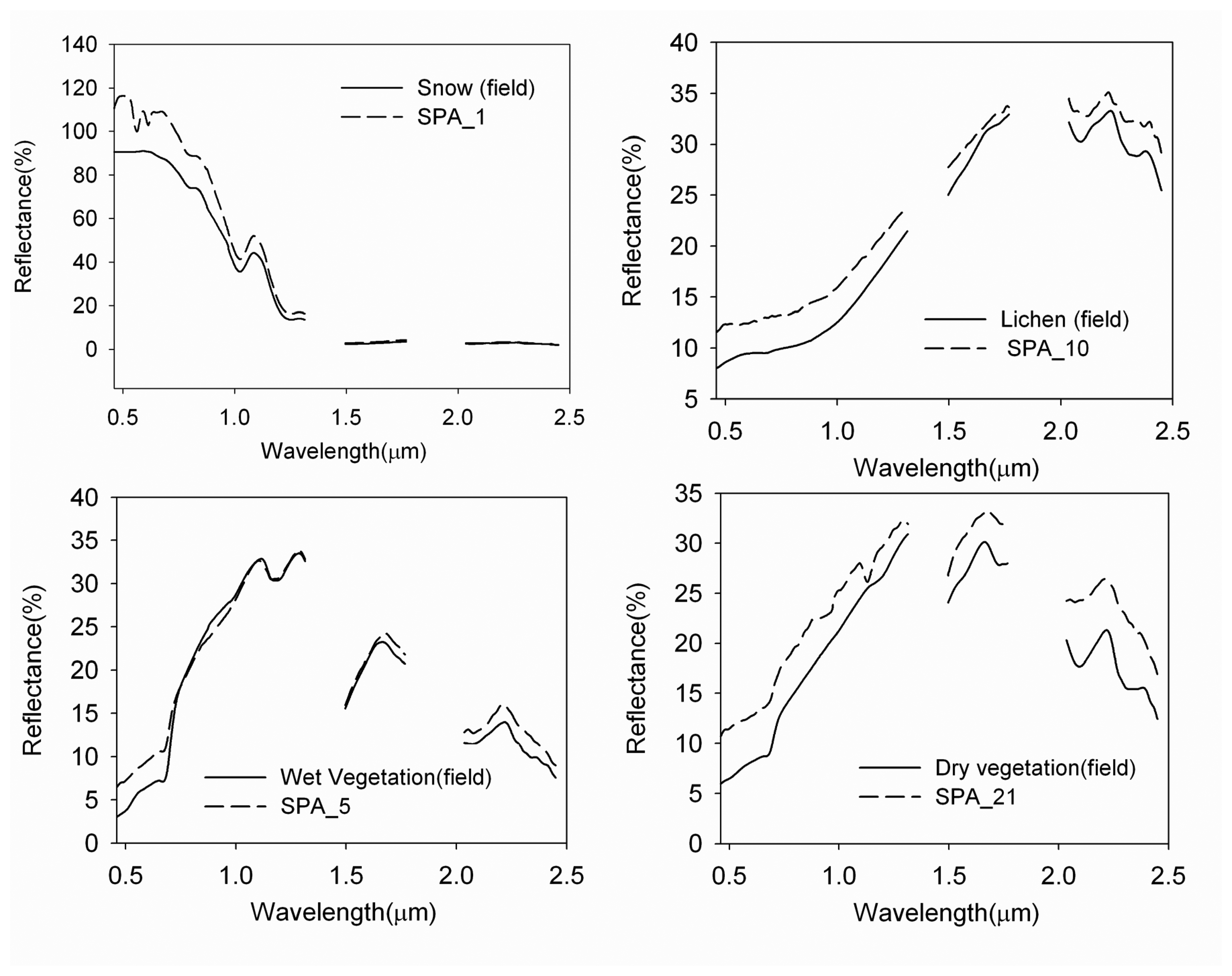
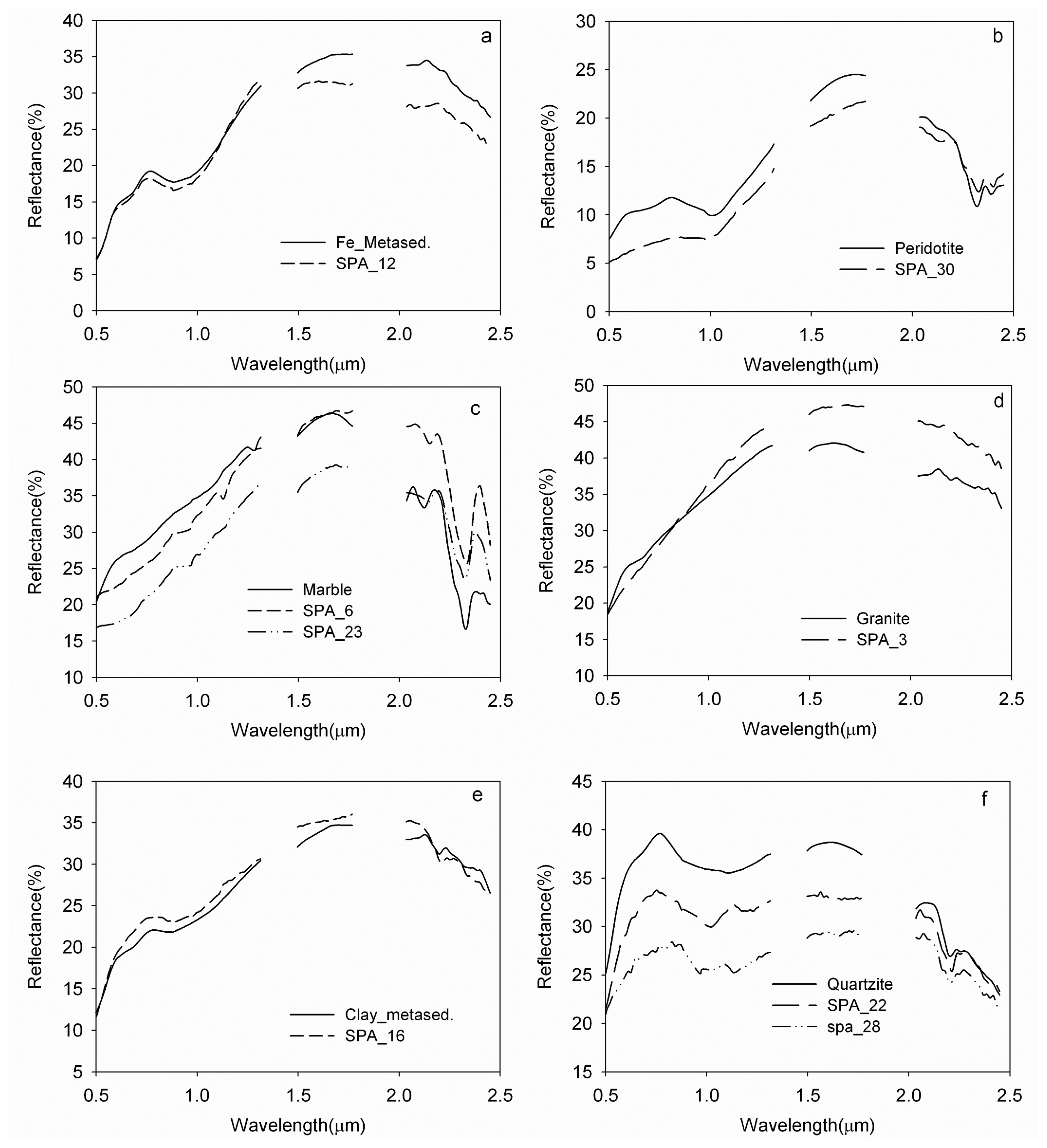
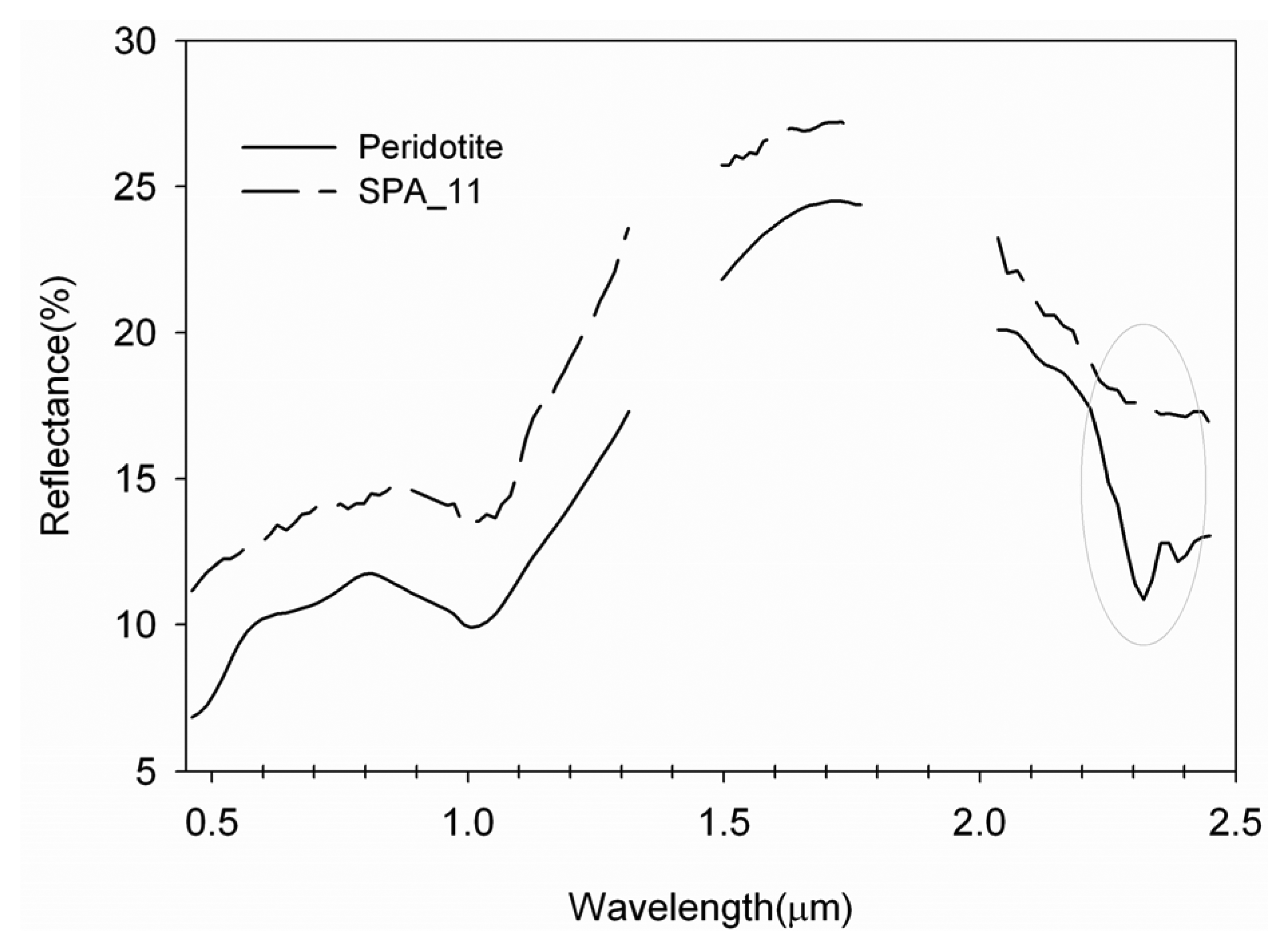
Comparison with spectra collected in the field

Out of thirty endmembers, twenty-one represent vegetation, water, snow and shadow (

Table 2. Summary of SPA endmembers derived for the Baffin Island site. The geological endmember are highlighted

SPA Endmember	Label
1, 4, 8, 9, 13, 14, 15, 17, 19, 20, 24, 26, 27	Snow
2	Water
3	Felsic (Granite/varnish)
5	Vegetation (wet)
6	Marble
7	Shade
10, 18, 25, 29	Lichen
11	Peridotite
12	Fe-metasediment
16	Clay-metasediment
21	Dry vegetation
22	Quartzite
23	Marble (low albedo)
28	Quartzite (low albedo)
30	Peridotite

). Examples for snow, vegetation and lichen with closely matched ground-based reflectance spectra are illustrated in Figure 6. The remaining nine endmembers are geological and belong to six rock types: Fe-rich metasediments, clay- metasediments, marble, felsic rock (varnish/granite), peridotite and quartzite (Figures 7,8; Table 2).

Eight geological endmembers (SPA_3, SPA_6, SPA_12, SPA_16, SPA_22, SPA_23, SPA_28 and SPA_30) closely match field spectra (Figure 7). The SPA_12 endmember correlates well with field spectra of Fe-metasediment characterized by a strong absorption feature near 0.9 μm attributed to goethite or hematite [44] (Figure 7a). In the field, this endmember also corresponds to the occurrence of gaussans. The SPA_30 is characterized by a broad ferrous-iron absorption feature at 0.93μm observed in spectra of pyroxene and hornblende [38] and a Fe,Mg-OH vibrational feature at 2.32μm, and is a close match to the field spectrum of peridotite (Figure 7b). SPA_6 and SPA_23 match the field spectrum of marble based on a strong carbonate (CO₃) feature near 2.30-2.35 μm, but they differ in overall spectral amplitude. For SPA_ 23 the carbonate feature is centered near 2.32 μm but for SPA_6 it lies near 2.34 μm. (Figure 7c). SPA_3 is a close match to the field spectrum of granite (Figure 7d) and represents multiple felsic targets with common spectral properties (e.g. overall higher reflectance and lack of obvious spectral absorption features). SPA_16 is another metasediment but it displays a clay absorption feature at 2.2 μm and a weak iron feature at 0.9μm (Figure 7e). Two endmembers spectrally similar but varying in amplitude, SPA_22 and SPA_28, are identified as quartzite based on a match with field spectra (Figure 7f).

We failed to find field spectra that closely match the endmember SPA_11. The closest match is peridotite (Figure 8), but this endmember lack the spectral absorption feature at 2.32μm that is observable in the SPA_30 peridotite endmember and field spectra (Figure 7b). The accurate identification of this endmember requires additional fieldwork.

Comparison with IEA image endmembers

We also performed a comparison between endmembers of geological interest derived from IEA and SPA (

Table 3. Comparison between IEA and SPA endmembers

Rock_type	IEA endmember	SPA endmember
Felsic (Granite/varnish)	IEA_3	SPA_3
Marble	IEA_7, IEA_22 (Similar but differ in amplitude)	SPA_6, SPA_23 (Similar but differs in amplitude)
Peridotite	IEA_14	*SPA_11, SPA_30
Fe-metasediment	IEA_19	SPA_12
Clay-metasediment	IEA_13	SPA_16
Metasediment	IEA_28	Missing
Quartzite	IEA_30	SPA_22, SPA_28 (Similar but differs in amplitude)

^*This endmember is labeled as peridotite based on Figure 8.

). For IEA the total number of endmembers was set to 30 and the spectral angle to 2.5 degrees. Results from both methods are comparable with two exceptions. First, SPA misses a endmember (metasediment) identified by IEA that has a good match with field spectra (Figure 9). In the second exception SPA extracts a second endmemember for peridotite (Figure 8). The endmember abundance maps (not shown) suggests that both peridotite endmembers map distinct spatial areas.

Changes in simplex volume

The change in the volume ratio (ν _ratio_l) between successive iterations is shown in Figure 10. The curve converges at endmember 24 ((ν _ratio₂₄= 1.24) after which the volume ratio remains less than 1.0. However, we found that endmembers of geological interest were extracted after endmember 24. For example, peridotite, an important rock type for the mining exploration of nickel, is extracted as the 30^th endmember. The majority of the snow, water, shade and vegetation endmembers were derived before this point, as shown in Table-2.

6. Discussion and future work

The SPA algorithm extracts endmembers from hyperspectral data without having to reduce the data dimensionality. It uses the spectral angle (alike IEA) and the spatial adjacency of pixels in the image to constrain the selection of candidate pixels representing an endmember. We designed SPA based on the observation that many targets have spatial continuity (e.g. bedrock lithologies) in hyperspectral imagery and thus a spatial constraint would be beneficial in the endmember search. We assumed that pixels that are spatially adjacent are more likely to have similar spectral properties and thus represent one endmember, and, that the probability that two adjacent pixels are both spurious is low. Experiments on two datasets demonstrate that SPA can effectively extract endmembers while requiring minimal user interaction.

It should be pointed out that the procedure to identify the simplex vertices in SPA is similar to that for advanced convex-based endmember selection methods such as MAX-D, VCA and SGA. However, of the convex-based endmember-search algorithms discussed in this paper, only SPA makes use of both the spectral angle and spatial adjacency to determine which pixels should form one endmember. By using the average of multiple pixels as one endmember, the SPA-derived endmember spectra appear less noisy (e.g. smoother), which is helpful for the improvement of unmixing results [45]. Given that spatially adjacent pixels are not likely of being simultaneously spurious, the use of the spatial adjacency makes SPA endmembers less sensitive to isolated noisy pixels, an inherent problem for convex–based endmember-search methods [21]. Although we initially designed SPA for geological applications (e.g. spatial continuity of bedrock), it offers potential for a variety of applications where the premise of spatial adjacency applies. Ecological examples include tree crowns and plant communities.

An additional product of the SPA is data describing the change of the simplex volume ratio between successive iterations during the endmember extraction. It illustrates the influence of a new endmember on the data structure, and provides information on the convergence of the algorithm. Though the rate of convergence speed can vary with the complexity of the scene, the patterns are similar showing the largest changes in volume ratio at the beginning of the endmember extraction process, followed by progressively smaller changes and convergence towards a plateau. If the endmember search terminates before the convergence point (the volume ratio is close to 1.0), significant endmembers will be missed. However as seen in the Baffin island example, endmembers for targets of interest may also be found beyond the convergence point. Thus additional research is required to properly constrain the number of endmember for a given search and application.

Comparison of endmembers obtained from SPA and IEA showed that both algorithms generate similar results (Table 2). Both methods operate on reflectance data, which is different from other algorithms such as VCA, N-FINDER and ICE that require a data dimensional reduction step. In the experiment with the Baffin island data, SPA missed one rock type (Metasediment), but obtained a additional rock endmember identified as a possible peridotite. Clearly different endmember-search algorithms can yield different endmember sets, indicating that the use of multiple search algorithms may reduce the chance of missing endmembers of interest.

The computation load of endmember-search algorithms is an important issue for the automatic extraction of endmembers, given the increasing volumes of hyperspectral data available. We did not study the computational efficiency of SPA, but because SPA is fundamentally similar to VCA and Max_D, that reported to be of high computational efficiency [14, 27], we believe the efficiency of SPA should be comparable. It takes about 35 minutes for SPA to extract 30 endmembers for a data cube of 512 pixels, 512 lines and 101 bands using a PC with PIV CPU (1.0GMHz) and 512M of RAM. This test is based on the current IDL implementation of SPA algorithm which has not been optimized for computational efficiency.

There are a number of potential improvements to SPA that require further research namely: 1) a means for the automatic determination of the spectral angle threshold (t _θ) and spatial threshold (t _pixel), and 2) a means to constrain the total number of the endmembers in the scene. In our experiments we found that 2.5 degrees for t _θ and 1 pixel for t _pixel provide good endmember estimates. However, the selection of t _pixel and t _θ should be scene dependent because of the varying spatial and spectral complexity in different data. Currently, the choice of these two thresholds is still arbitrary and it would valuable to develop a more robust way to define values for t _θt_pixel. Finally, we do not yet have a definite means of constraining the number of endmembers in a given search, though the simplex volume change during the search offers a qualitative assessment. The concept of virtual dimensionality (VD) has been proposed and proven useful for this purpose in recent years [18, 46]. The use of the VD concept within SPA may allow the study of the relationship between VD and simplex volume in the future and prove valuable to constrain the number of endmembers.

References and Notes

1. Clark, R.N.; Gallagher, A.J.; Swayze, G.A. Material absorption band depth mapping of imaging spectrometer data using a complete band shape least-squares fit with library reference spectra. In Proceedings 2ndAirborne Visible/Infrared Imaging Spectrometer (AVIRIS) Workshop; JPL Publication; Volume 90-54, 1990; pp. 176–186. [Google Scholar]
2. Kruse, F. A.; Huntington, J. H. The 1995 Geology AVIRIS Group Shoot. Proceedings of the Sixth Annual JPL Airborne Earth Science Workshop, JPL publication 96-4 1996, 1, 155–166. [Google Scholar]
3. Ben-Dor, E.; Kruse, F.A. Surface mineral mapping of Makhtesh Ramon Negev, Israel using GER 63 channel scanner data. International Journal of Remote Sensing 1995, 16, 3529–3553. [Google Scholar]
4. Mustard, J.F.; Pieters, C.M. Abundance and distribution of ultramafic microbreccia in Moses Rock dike: Quantitative application of mapping spectroscopy. Journal of Geophysical Research 1987, 92(B10), 10376–10390. [Google Scholar]
5. Murphy, R.J. Mapping of jasperiod in the Cedar Mountains, Utah, U.S.A., using imaging spectrometer data. International Journal of Remote Sensing 1995, 16, 1021–1041. [Google Scholar]
6. Bierwirth, P.; Blewett, R.; Huston, D. Finding new mineral prospects with HYMAP: early results from a hyperspectral remote-sensing case study in the west Pilbara. AGSO Research Newsletter. 31 November 1999. http://www.ga.gov.au/pdf/Corp0038.pdf.
7. Asner, G.P.; Heidebrecht, K.B. Spectral unmixing of vegetation, soil and dry carbon cover in arid regions: comparing multispectral and hyperspectral observations. International Journal of Remote Sensing 2002, 23, 3939–3958. [Google Scholar]
8. Neville, R.A.; Levesque, J.; Staenz, K.; Nadeau, P.; Hauff, P.; Borstad, G.A. Spectral unmixing of hyperspectral imagery for mineral exploration: comparison of results from SFSI and AVIRIS. Canadian Journal of Remote Sensing 2003, 29, 99–110. [Google Scholar]
9. Adams, J.B.; Gillespie, A. R. Remote sensing of landscapes with spectral images: A physical modeling approach; Cambridge University Press: New York, 2006; p. 362. [Google Scholar]
10. Boardman, J. W.; Kruse, F. A.; Green, R. O. Mapping target signatures via partial unmixing of AVIRIS data. In Summaries, Fifth JPL Airborne Earth Science Workshop; JPL Publication 95-1, 1995; vol. 1, pp. 23–26. [Google Scholar]
11. Boardman, J.W. Automating spectral unmixing of AVIRIS data using convex geometry concepts. Summaries of the fourth Annual JPL airborne Geoscience Workshop, JPL Publication 93-26 1993, vol. 1, 11–14. [Google Scholar]
12. Winter, M. E. N-FINDR: An algorithm for fast autonomous spectral end-member determination in hyperspectral data. Descour, M. R., Shen, S. S., Eds.; Imaging Spectrometry V; In Proceedings of SPIE; vol. 3753, 1999; Denver, USA; pp. 266–275. [Google Scholar]
13. Neville, R. A.; Staenz, K.; Szeredi, T.; Lefebvre, J.; Hauff, P. Automatic endmember extraction from hyperspectral data for mineral exploration. In Proceedings of Fourth International Airborne Remote Sensing Conference and Exhibition / 21st Canadian Symposium on Remote Sensing; vol. 2, Ottawa, Canada, 1999; pp. 891–897. [Google Scholar]
14. Nascimento, J.M.P.; Dias, J.M.B. Vertex component analysis: a fast algorithm to unmix hyperspectral data. IEEE Transactions on Geoscience and Remote Sensing 2005, 43, 898–910. [Google Scholar]
15. Bajorski, P.; Schott, J.; Ientilucci, E. Comparison of Basis-Vector Selection Methods for Target and Background Subspaces as Applied to Subpixel Target Detection. Shen, S. S., Lewis, P. E., Eds.; In Algorithms and Technologies for Multispectral, Hyperspectral, and Ultraspectral Imagery X, Proceedings of SPIE; vol. 5425, Orlando, USA, 2004; pp. 97–108. [Google Scholar]
16. Gruninger, J. H.; Ratkowski, A. J.; Hoke, M. L. The sequential maximum angle convex cone (SMACC) endmember model. Shen, S. S., Lewis, P. E., Eds.; In Algorithms and Technologies for Multispectral, Hyperspectral, and Ultraspectral Imagery X, Proceedings of SPIE; Volume 5425, Orlando, USA, 2004; pp. 1–14. [Google Scholar]
17. Berman, M.; Kiiveri, H.; Lagerstrom, R.; Ernst, A.; Dunne, R.; Huntington, J. 2004. ICE: An automated statistical approach to identifying endmembers in hyperspectral images. IEEE Transactions on Geoscience and Remote Sensing 2004, 42, 2085–2095. [Google Scholar]
18. Chang, C.-I.; Wu, C.-C.; Liu, W.-W.; Ouyang, Y.-C. A new growing method for simplex-based endmember extraction algorithm. IEEE Transactions on Geoscience and Remote Sensing 2006, 44, 2804–2819. [Google Scholar]
19. Miao, L.; Qi, H. Endmember extraction from highly mixed data using minimum volume constrained nonnegative matrix factorization. IEEE Transactions on Geoscience and Remote Sensing 2007, 45, 765–777. [Google Scholar]
20. Bowles, J. H.; Palmadesso, P. J.; Antoniades, J. A.; Baumback, M. M.; Rickard, L. J. Use of filter vectors in hyperspectral data analysis. Strojnik, M., Andresen, B. F., Eds.; In Infrared Spaceborne Remote Sensing, Proceedings of SPIE; vol. 2553, San Diego, USA, 1995; pp. 148–157. [Google Scholar]
21. Howes, D. J.; Clare, P. E.; Oxford, W. J.; Murphy, S. Endmember selection techniques for improved spectral unmixing. Shen, S. S., Lewis, P. E., Eds.; In Algorithms and Technologies for Multispectral, Hyperspectral, and Ultraspectral Imagery X, Proceedings of SPIE, vol. 5425; Orlando, USA; vol. 5425, 2004; pp. 65–76. [Google Scholar]
22. Rogge, D.; Rivard, B.; Zhang, J.; Harris, J.; Feng, J.; Sanchez, A. Integration of spatial-spectral information for the improved extraction of endmembers. Remote Sensing of Environment 2007, 110, 287–303. [Google Scholar]
23. Haskell, K.H.; Hanson, R. J. An algorithm for linear least squares problems with equality and non-negativity constraints. Mathematical Programming 1981, 21, 98–118. [Google Scholar]
24. Shimabukuro, Y.E.; Smith, J.A. The least squares mixing models to generate fraction images derived from remote sensing on multispectral Data. IEEE Transactions on Geoscience and Remote Sensing 1991, 29, 16–20. [Google Scholar]
25. Bajorski, P. Stepwise simplex projection method for the selection of endmembers in hyperspectral images. Shen, S. S., Lewis, P. E., Eds.; In Algorithms and Technologies for Multispectral, Hyperspectral, and Ultraspectral Imagery XI, Proceedings of SPIE; Volume 5806, Orlando, USA, 2005; pp. 318–329. [Google Scholar]
26. Gritzmann, P.; Klee, V. On the Complexity of Some Basic Problems in Computational Convexity: II. Volume and Mixed Volumes. In Technical Report TR94 -31; DIMACS, Rutgers University: New Brunswick, NJ, 1994. [Google Scholar]
27. Winter, M. E. A proof of the N-FINDR algorithm for the automated detection of end-members in a hyperspectral image. Shen, S. S., Lewis, P. E., Eds.; In Algorithms and Technologies for Multispectral, Hyperspectral, and Ultraspectral Imagery XI, Proceedings of SPIE; Orlando, USA; Vol. 5425, 2004; pp. 31–41. [Google Scholar]
28. Lee, K. A subpixel scale target detection algorithm for hyperspectral imagery. PhD. dissertation, Rochester Institute of Technology, 54 Lomb Memorial Drive, Rochester, NY, 2003. [Google Scholar]
29. Green, A.A.; Berman, M.; Switzer, P.; Craig, M.D. A transformation for ordering multispectral data in terms of image quality with implications for noise removal. IEEE Transactions on Geoscience and Remote Sensing 1988, 26, 65–74. [Google Scholar]
30. Plaza, A.; Martinez, P.; Perez, R.; Plaza, J. A quantitative and comparative analysis of endmember extraction algorithms from hyperspectral data. IEEE Transactions on Geoscience and Remote Sensing 2004, 42, 650–663. [Google Scholar]
31. Plaza, A.; Chang, C. An improved N-FINDER algorithm in Implementation. Shen, S. S., Lewis, P. E., Eds.; In Algorithms and Technologies for Multispectral, Hyperspectral, and Ultraspectral Imagery XI, Proceedings of SPIE; vol. 5806, Orlando, USA, 2005; pp. 298–306. [Google Scholar]
32. Turner, J.F., II; Zhang, J.; O'Connor, A. A spectral identity mapper for chemical image analysis. Applied spectroscopy 2004, 58, 1308–1317. [Google Scholar]
33. Grande, B.; Manne, R. Use of convexity for finding pure variables in two-way data from mixtures. Chemometrics and intelligent laboratory systems 2000, 50, 19–33. [Google Scholar]
34. Gao, B.C.; Goetz, A.F.H. Column atmospheric water vapor and vegetation liquid water retrievals from airborne imaging spectrometer data. Journal of Geophysical Research 1990, 95, 3549–3564. [Google Scholar]
35. Boardman, J. W. Post-ATREM polishing of AVIRIS apparent reflectance data using EFFORT: a lesson in accuracy versus precision. In Summaries of the Seventh JPL Airborne Earth Science Workshop; JPL Publication 99-17, 1998; vol. 1, p. 53. [Google Scholar]
36. Abrams, M.J.; Ashley, R.P.; Rowan, L.C.; Goetz, A.F.H.; Kahle, A.B. Mapping of hydrothermal alteration in the Cuprite Mining District, Nevada, using aircraft scanner images for the spectral region 0.46–2.36μm. Geology 1977, 5, 713–718. [Google Scholar]
37. Kruse, F.A.; Kierein-Young, K. S.; Boardman, J. W. Mineral mapping at Cuprite, Nevada with a 63 channel imaging spectrometer. Photogrammetric Engineering and Remote Sensing 1990, 56, 83–92. [Google Scholar]
38. Hook, S.J.; Rast, M. Mineralogic mapping using Airborne Visible Infrared Imaging Spectrometer (AVIRIS), Shortwave Infrared (SWIR) data acquired over Cuprite, Nevada. Green, R.O., Ed.; In Proceedings of the Second Airborne Visible Infrared Imaging Spectrometer (AVIRIS) Workshop, JPL Publication 90-54; 1990; pp. 199–207. [Google Scholar]
39. Clark, R.N.; Swayze, G.A.; Gallagher, A. Mapping Minerals with Imaging Spectroscopy. U.S. Geological Survey, Office of Mineral Resources Bulletin 1993, 2039, 141–150. [Google Scholar]
40. Swayze, G.A.; Clark, R.N.; Kruse, F.; Sutley, S.; Gallagher, A. Ground-Truthing AVIRIS Mineral Mapping at Cuprite, Nevada. Summaries of the Third Annual JPL Airborne Geosciences Workshop, Volume 1: AVIRIS Workshop. JPL Publication 92-14 1992, 47–49. [Google Scholar]
41. Lewry, J.F.; Stauffer, M.R. The early Proterozoic Trans-Hudson Orogen of North America; Geological Association of Canada, 1990; Vol. 37, p. 505. [Google Scholar]
42. St-Onge, M.R.; Wodicka, N.; Lucas, S.B. Geology of McKeller Bay-Wight Inlet – Frobisher Bay area, southern Baffin Island, Northwest Territories: Current Research, 1998-C. Geological Survey of Canada 1999, 43–53. [Google Scholar]
43. St-Onge, M.R.; Wodicka, N.; Scott, D.J. Review of crustal architecture and evolution in the Ungava Peninsula – Baffin Island area: connection to the lithoprobe ECSOOT transect. Canadian Journal of Earth Sciences 2002, 39, 589–610. [Google Scholar]
44. Clark, R.N.; Swayze, G.A.; Livo, K.E.; Kokaly, R.F.; Sutley, S.J.; Dalton, J.B.; McDougal, R.R.; Gent, C.A. Imaging spectroscopy: Earth and planetary remote sensing with the USGS Tertracorder and expert systems. Journal of Geophysical Research 2003, 108(E12), 5-1–5-14. [Google Scholar]
45. Clark, R. N. Chapter 1: Spectroscopy of Rocks and Minerals, and Principles of Spectroscopy. In in Manual of Remote Sensing, Volume 3, Remote Sensing for the Earth Sciences; Rencz, A.N., Ed.; John Wiley and Sons: New York, 1999. [Google Scholar]
46. Barducci, A.; Mecocci, A. Theoretical and experimental assessment of noise effects on least-squares spectral unmixing of hyperspectral images. Optical Engineering 2005, 44, 087008-1–087008-17. [Google Scholar]
47. Chang, C.-I. Hyperspectral imaging : Techniques for spectral detection and classification; Plenum Publishing Co., 2003; p. 370p. [Google Scholar]
Figure 1. Regional geology of south-western Baffin Island and zoom of local geology of the study area (1:100 000) (modified from St-Onge et al., 1999).
Sensors 08 01321f1
Figure 2. Probe 1 hyperspectral data of the study area. Circles represent ground locations where field spectra and samples were collected.
Sensors 08 01321f2
Figure 3. Comparison between SPA endmember and PPI endmember(“true”endmember). The solid lines denotes PPI endmembers.
Sensors 08 01321f3
Figure 4. Comparison of SPA and SMACC endmembers. a) endmember representatives of the same target (zeolite), b) SMACC endmember capturing noise
Sensors 08 01321f4
Figure 5. Convergence of SPA for the Cuprite data. The arrow marks the last iteration where the simplex volume ratio for successive iterations exceeds 1.0.
Sensors 08 01321f5
Figure 6. Endmember spectra for snow, vegetation and lichen. The dashed lines are the SPA-endmembers, and the solid lines are the corresponding closely matched field spectra. The strong water absorption features near 1.4 and 1.9 um were discarded because of low signal.
Sensors 08 01321f6
Figure 7. Comparison of SPA geological endmembers and field spectra. The strong water absorption features near 1.4 and 1.9 um were discarded because of low signal.
Sensors 08 01321f7
Figure 8. Comparison between the SPA_11 endmember and field spectrum of peridotite. The circle marks the region where absorption feature is present on the field spectrum of peridotite but absent from the SPA_11.
Sensors 08 01321f8
Figure 9. The endmember found by IEA but not by SPA. The solid line is a field spectrum for metasediment, the dashed line is the IEA endmember.
Sensors 08 01321f9
Figure 10. Convergence of the SPA for the Baffin data The arrow marks the last iteration where the simplex volume ratio for successive iterations exceeds 1.0.
Sensors 08 01321f10