Can ISO-Defined Urban Sustainability Indicators Be Derived from Remote Sensing: An Expert Weighting Approach

 , ,
, ,  and
and
Abstract
:1. Introduction
2. Theoretical Background
2.1. Sustainable Urban Development
2.2. Indicators for the Sustainable Development of Communities
2.3. Remote Sensing and Sustainability
2.4. Indicators for Sustainable Development of Communities and Remote Sensing
2.5. Gathering the Remote Sensing Experts’ Knowledge
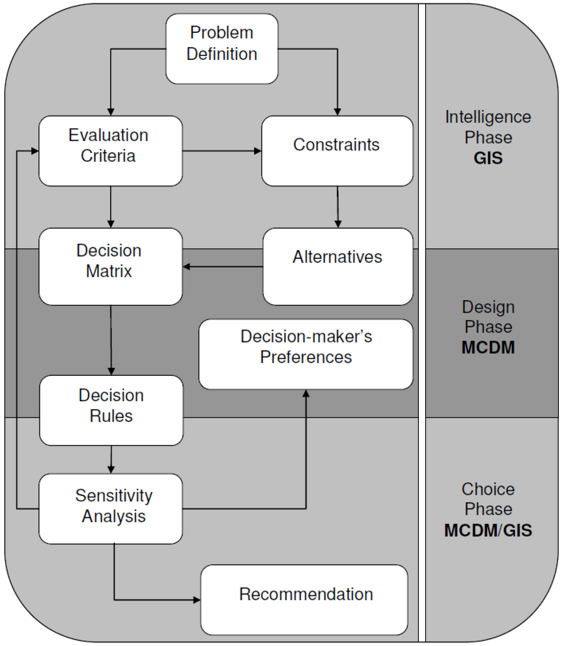
2.6. Multi-Criteria Decision-Making
- A goal or a set of goals the decision maker (interest group) attempts to achieve;
- The decision maker or group of decision makers involved in the decision-making process along with their preferences with respect to evaluation criteria;
- A set of evaluation criteria (objectives and/or attributes) based on which the decision makers evaluate alternative courses of action;
- The set of decision alternatives, that is, the decision or action variables;
- The set of uncontrollable variables or states of nature (decision environment); and
- (1)
- The Intelligence Phase focuses on defining the problem definition that incorporates the evaluation criteria and constraints (restrictions). MCDM problems are hierarchically structured and consist of an overall object and several sub-objectives. Each sub-objective can be further divided into additional sub-objectives and finally their criteria at the bottom level. The structure of the problem definition always depends on the research question and the application domain. The selection of evaluation criteria can be realized by examining relevant literature, incorporating domain experts, and conducting analytical studies or surveys.
- (2)
- Within the scope of the Design Phase, the decision matrix can be generated for each hierarchical level that includes the criteria, the alternatives, and the criterion weights. In general, weights express the preferences of the decision makers for the criteria that are incorporated in the decision model and represent the relative importance of each criterion with respect to others. High weight values indicate a strong influence of the particular criterion. Mathematical methods to retrieve the set of criterion weights are ranking-, rating-, pairwise comparison-, trade-off analysis- or entropy-based criterion weight methods, which can be further divided into global- and local methods [14,17,18].
- (3)
- In regard to the Choice Phase, the estimated criterion weights are used as input to apply specific decision rules to rank the alternatives with respect to their performance. Additionally, sensitivity analysis methods have to be performed to verify the robustness and stability of the decision model outputs. The result of the decision-making process is a recommendation for future action.
3. Methodology
- Questionnaire: online survey
- Analytical Hierarchy Process (AHP) after Saaty, 1980 [19].
3.1. Selection of the QoL Indicators with Remote Sensing Potential
- Energy consumption of public buildings per year (kWh/m2): Total use of electricity at final consumption stage by public buildings (kWh) within a city divided by total floor space of these buildings in square meters (m2).
- Total electrical energy-use per capita (kWh/year): Total electrical usage of a city in kilowatt-hours including residential and non-residential use divided by the total population of the city.
- Noise pollution: mapping the noise level (day-evening-night) likely to cause annoyance as given in ISO 1996-2:1987, identifying the areas of the city where is greater than 55 dB(A), and estimating the population of those areas as a percentage of the total city population.
- Square meters of public outdoor recreation space per capita: The square meters of indoor public recreation space divided by the population of the city.
- Percentage of city population living in slums: The number of people living in slums divided by the city population.
- Percentage of households that exist without registered legal titles: The number of households that exist without registered legal titles divided by the total number of households.
- The amount of the city’s solid waste that is disposed of in a sanitary landfill in tons divided by the total amount of solid waste produced in the city in tons.
- Kilometers of high capacity public transport system per 100,000 population: The kilometers of high capacity public transport systems operating within the city divided by 1/100,000th of the city’s total population.
- Number of personal automobiles per capita: Total number of registered personal automobiles in a city divided by the total city population.
- Green area (hectares) per 100,000 population: Total area (in hectares) of green in the city divided by 1/100,000th of the city’s total population.
- Areal size of informal settlements as a percent of city area: The area of informal settlements in square kilometers (numerator) divided by the city area in square kilometers.
- Land area (Square kilometers).
- Percentage of non-residential area (square kilometers).
3.2. Questionnaire-Based Approach: The Online Survey
3.2.1. Concept Development
3.2.2. Analysis of the Responses from the Online Questionnaire
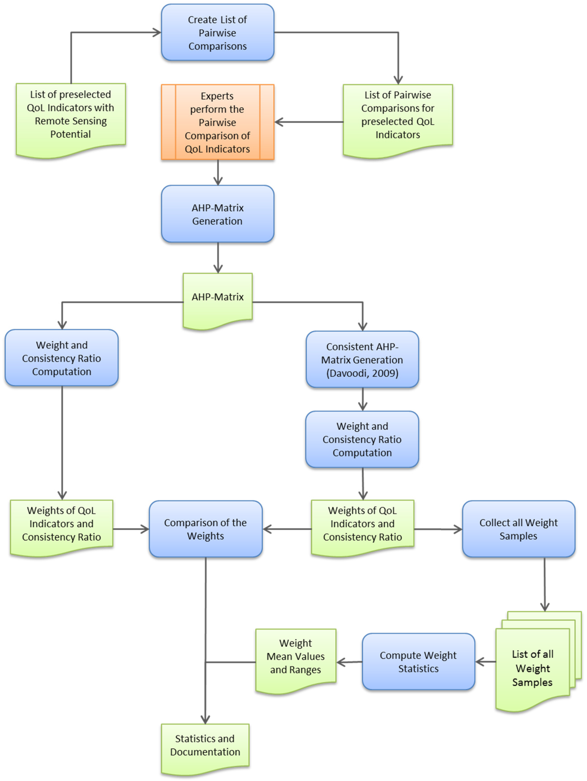
3.3. Pairwise Comparison Approach: AHP
3.3.1. Concept Development for the AHP Matrix Calculations
- (i)
- For each hierarchical level of the MCDM model, a squared matrix is generated that incorporates n2 elements, which represent all possible pairwise combinations for the criteria of a certain hierarchical level. The diagonal of the matrix and all elements below the diagonal are excluded for retrieving the pairwise comparison values from the involved experts. Therefore, the number of comparisons is reduced to actual pairwise comparisons. The experts have to rate their preferences according to the scale of [19], where the values range from 1 (same importance) to 9 (extreme importance). The diagonal of the matrix will be filled with ones, because self-comparisons must be equally rated. Finally, the matrix below the diagonal are filled with the reciprocal values of the expert preferences by changing the values of the row and column indices of the matrix.
- (ii)
- Concerning the calculation of the weights, the initial pairwise comparison matrix is multiplied by itself. For each row, the sum is calculated and normalized. The normalized values represent the calculated eigenvector from the pairwise comparisons of relative importance. This procedure is performed for several iterations until no changes of the criterion weights can be identified anymore. The number of iterations depends on the desired accuracy (the number decimal place). An approximation approach for calculating the criterion weights can be found in Malczewski, 1999 [14].
- (iii)
- This step illustrates the consistency check of the pairwise comparisons. Each column of the initial pairwise comparison matrix is multiplied with the corresponding element of the weighted sum vector (Step ii). Afterwards, for each row, the sum is computed (weighted sum vector). During the next task, the consistency vector has to be determined by dividing the weighted sum vector by the criterion weights (Step ii). The average value of the consistency vector is greater or equal (full consistency) to the number of criteria and will be normalized by the following formula, representing the Consistency Index (CI):
3.3.2. Analysis of the Responses from the Pairwise Comparisons (Analytical Hierarchy Process)
- (1)
- For each row of the inconsistent AHP matrix, a consistent AHP matrix will be generated.
- (a)
- The row vector according to the row index i is copied to the consistent AHP matrix.
- (b)
- The reciprocals of the row vector are inserted into the column vector by changing the order of the row i and column index j.
- (c)
- The values of the diagonal w[i, j] are equal to one (indices i and j are equal).
- (d)
- The remaining elements of the consistent AHP matrix are calculated as follows w[i, j] = w[i, k] × w[k, j], where k represents the index of the initial row (step a).
- (2)
- All intermediate matrices, 13 in our case, are combined with the help of the geometric mean. The final matrix represents a consistent AHP matrix. For all intermediate matrices and the final matrix, the consistency is equal to zero, and all eigenvalues are equal to the number of indicators.
4. Results
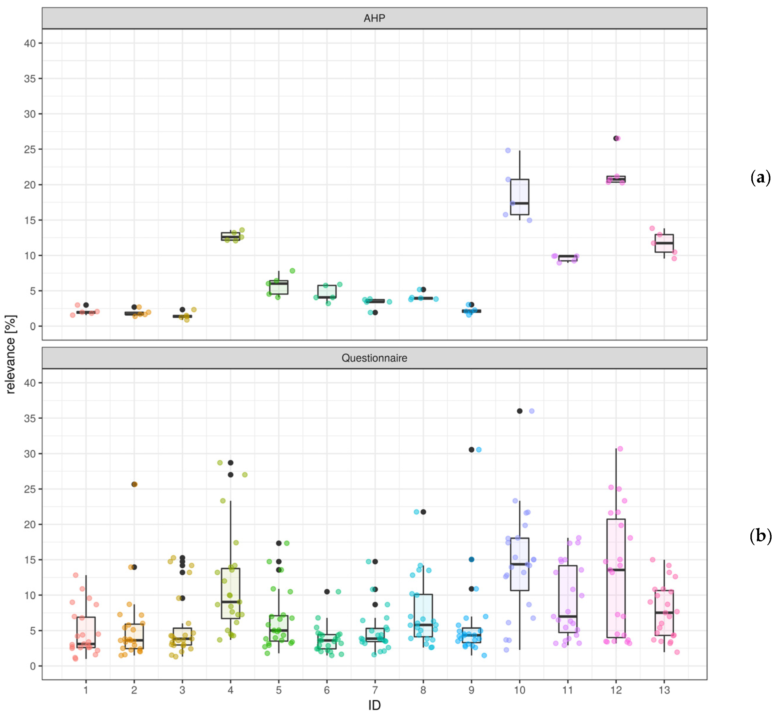
4.1. Evaluation of the Results of the Online Questionnaire
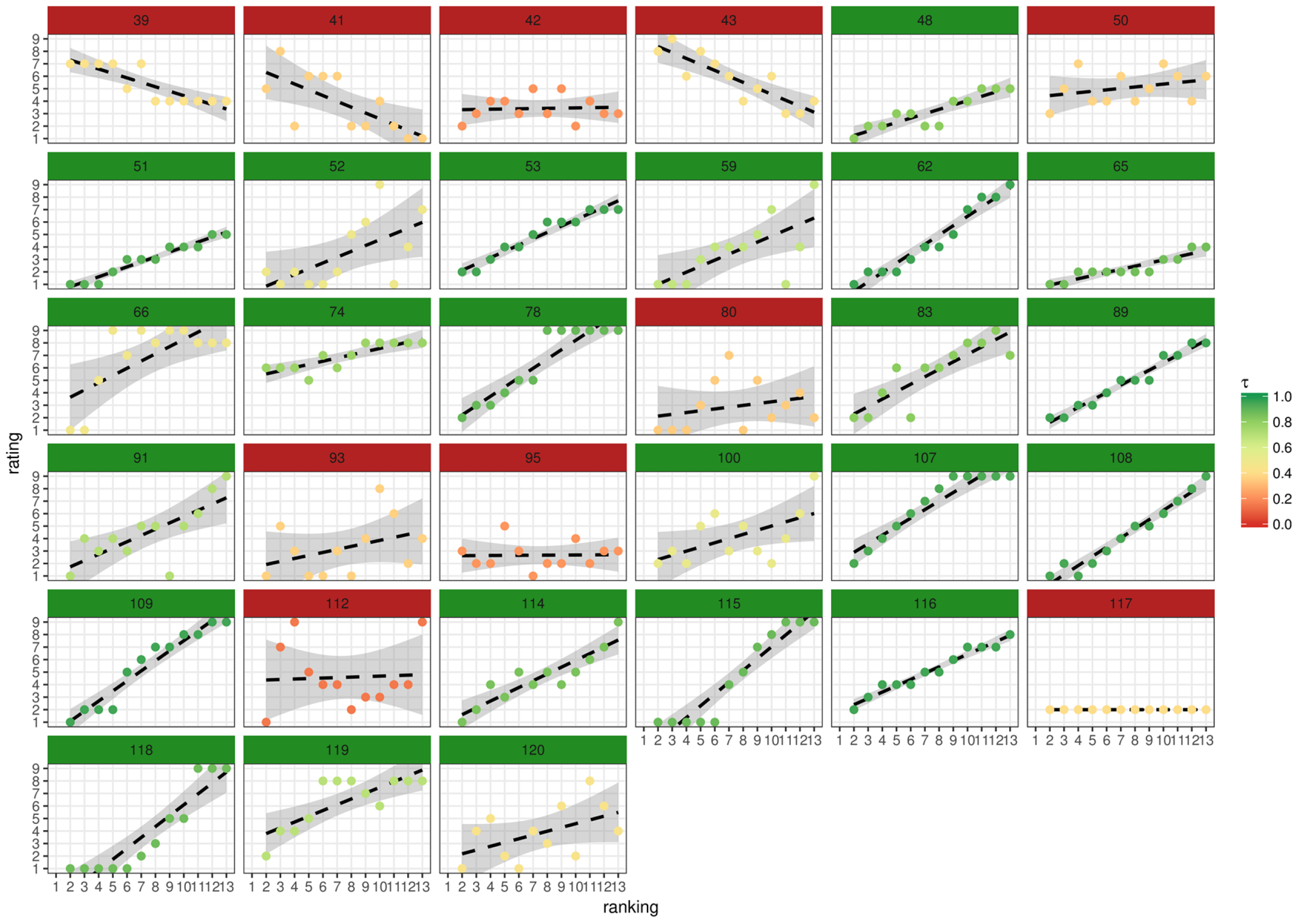
4.2. Evaluation of the Results from the Pairwise Comparison (AHP Approach)
5. Discussion
- (14) Academic university: i.a. PhD students, university professors
- Academic—extra-faculty (non-university) research institutes
- Engineering office/Engineering consultant: i.a. one software developer
- Public service
5.1. Proposals for Supplementary Indicators (Online Questionnaire Approach)
5.2. Identification of the Indicators That Are Best Suited for Assessment by Remote Sensing
5.3. Pros and Cons of the Assessment Approaches
5.4. Comparison of the Approaches (Online Questionnaire vs. AHP)
5.5. Potential Challenges in Applying of the Indicators that Are Best Suited for Assessment by Remote Sensing
6. Conclusions
7. Outlook
Acknowledgments
Author Contributions
Conflicts of Interest
Appendix A

- Q01: We ask for the professional background of the remote sensing expert.
- Q02: We ask for the professional experience with remote sensing and remote sensing derived data.
- Q03: Within this question, the 13 indicators are presented to the remote sensing expert. The expert has to rank the indicators according to their remote sensing relevance (Figure A2).

- Q04: After ranking the 13 indicators, they are again presented to the expert including the assigned ranks (Figure A3). The expert is asked if he agrees with the given ranking and the presented indicators in general. Within a non-obligatory comment box, the expert has the possibility to state the absence of an indicator. Indicators provided by the remote sensing experts in this way will not be included for the subsequent questions.
- Q05: Within the next step, the expert is asked to compare the remote sensing relevant indicator that he or she ranked highest with the other 12 indicators. The comparison is done by stating a number from 1 to 9 by use of a slider, where 1 means that the indicator that was ranked highest in Q03 is equally relevant when compared to another one and the numbers 2 to 9 mean that the indicator that was ranked highest is more relevant when compared to another one within the respective degree (Figure A4).
- Q06: In the following step, the calculation of the weights—that was done based on the values of the comparison in Q05—is presented to the remote sensing expert. He or she is asked for doing a plausibility check, i.e., he or she has to evaluate if the calculated weights correspond to the experts’ knowledge and experience. The expert has to state whether he or she agrees/disagrees on the distribution of the calculated weights and their respective values by clicking “Yes” or “No”, respectively (Figure A5). If the expert marks “No”, he or she is able to modify the values of the calculated weights manually in a next step. The online survey is split up into two groups here, namely the group of these experts who accept the calculation and those who deny the calculation and modify the values manually based on their expert knowledge.


- (Q09) where they are able to leave a comment about the survey, their experience with it or general suggestions and remarks.
- Q07: Experts that disagreed on the calculated weights are able to modify them within the following step (Figure A6). For each indicator, it is possible to enter values, while the sum of all indicators has to result in 100% and one indicator cannot have more than 88% on its own. It is not obligatory to enter numbers, thus it is also possible to continue without stating any number at all.
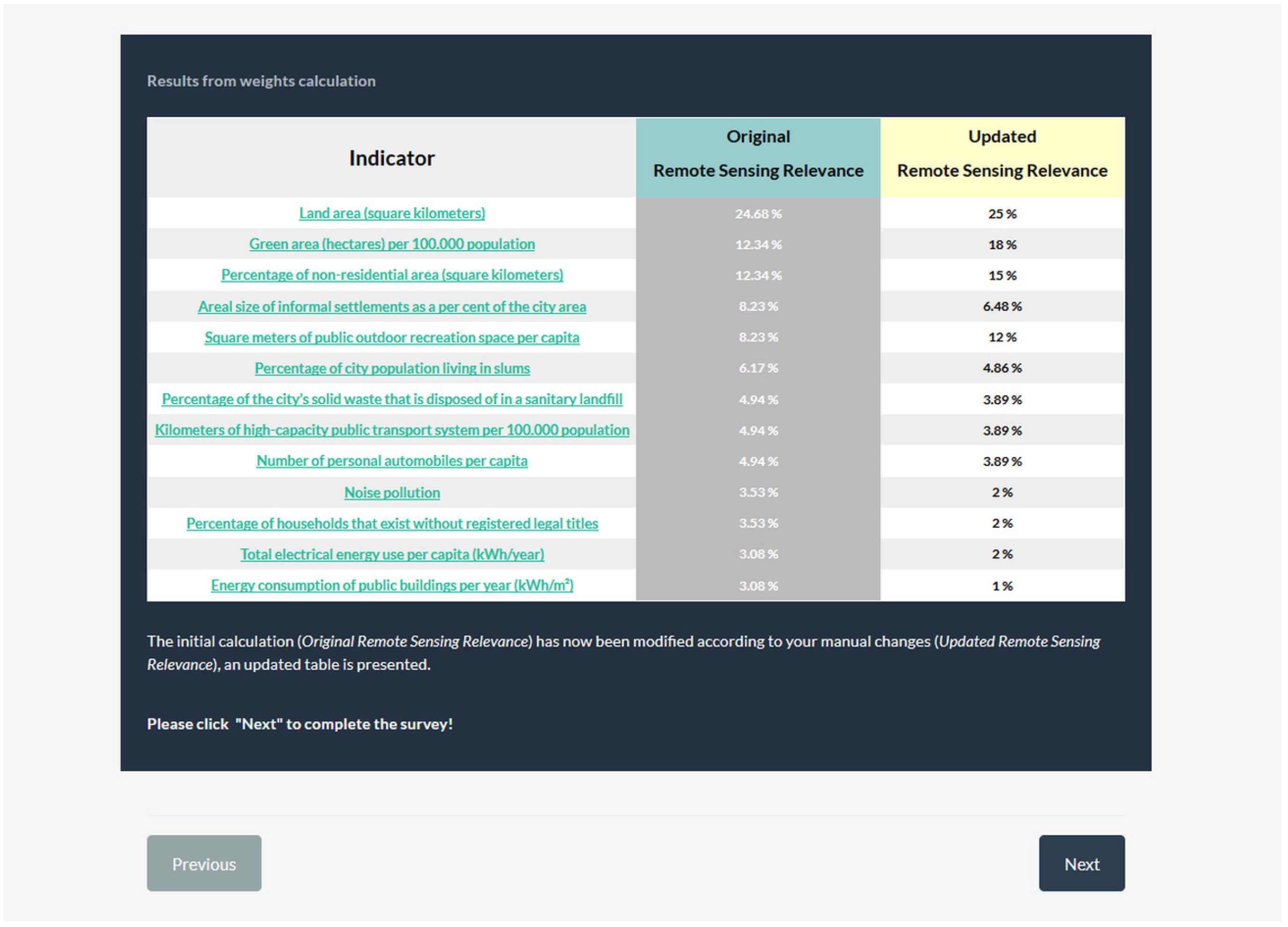
- Q08: After the confirmation (“Next”) of the modifications, the calculated weights including the experts’ modifications are once again presented to the remote sensing expert. These results are compared in a table next to the results of the initial calculation and may be evaluated by the remote sensing expert (Figure A7). If the expert again disagrees on the weight calculation that included his or her modifications, it is possible to return to the previous question (Q07) and modify the weights once again by clicking “Back”. If the expert agrees on the calculated weights based on the previously stated modifications, he or she reaches the end of the survey (Q09) where it is possible to leave a comment about the survey, the expert’s experience with it or general suggestions and remarks.


References
- ISO. ISO-Standard 37120:2014: Sustainable Development of Communities—Indicators for City Services and Quality of Life; ISO: Geneva, Switzerland, 2014. [Google Scholar]
- Blanco, H.; Wautiez, F.; Llavero, A.; Riveros, C. Sustainable development indicators in Chile: To what extent are they useful and necessary? Eure-Rev. Latinoam. Estud. Urbano Reg. 2001, 27, 85–95. [Google Scholar]
- Mahi, P. Developing environmentally acceptable desalination projects. Desalination 2001, 138, 167–172. [Google Scholar] [CrossRef]
- Trinder, J.C. Remote sensing for assessing environmental impacts based on sustainability indicators. In Proceedings of the International Archives of the Photogrammetry, Remote Sensing and Spatial Information Sciences, Beijing, China, 3–11 July 2008. [Google Scholar]
- Masser, I. Managing our urban future: The role of remote sensing and geographic information systems. Habitat Int. 2001, 25, 503–512. [Google Scholar] [CrossRef]
- Weng, Q. Remote Sensing for Sustainability; CRC Press: Boca Raton, FL, USA, 2016. [Google Scholar]
- Netzband, M.; Stefanov, W.L.; Redman, C. Applied Remote Sensing for Urban Planning, Governance and Sustainability; Springer Science & Business Media: Berlin, Germany, 2007. [Google Scholar]
- Rahman, A. Application of remote sensing and GIS technique for urban environmental management and sustainable development of Delhi, India. In Applied Remote Sensing for Urban Planning, Governance and Sustainability; Springer: Berlin, Germany, 2007; pp. 165–197. [Google Scholar]
- Kadhim, N.; Mourshed, M.; Bray, M. Advances in remote sensing applications for urban sustainability. Euro-Mediterr. J. Environ. Integr. 2016, 1, 7. [Google Scholar] [CrossRef]
- Esch, T.; Taubenböck, H.; Heldens, W.; Thiel, M.; Wurm, M.; Geiß, C.; Dech, S. Urban remote sensing—how can earth observation support the sustainable development of urban environments? In Proceedings of the Real CORP, Wien, Austria, 18–20 May 2010; pp. 1–11. [Google Scholar]
- Jain, M.; Knieling, J. Stadtentwicklung am Beispiel Indien: Empfehlungen aus planerischer Perspektive. In Globale Urbanisierung; Springer: Berlin, Germany, 2015; pp. 277–279. [Google Scholar]
- Azapagic, A.; Perdan, S. An integrated sustainability decision-support framework Part I: Problem structuring. Int. J. Sustain. Dev. World Ecol. 2005, 12, 98–111. [Google Scholar] [CrossRef]
- Azapagic, A.; Perdan, S. An integrated sustainability decision-support framework Part II: Problem analysis. Int. J. Sustain. Dev. World Ecol. 2005, 12, 112–131. [Google Scholar] [CrossRef]
- Malczewski, J. GIS and Multicriteria Decision Analysis; John Wiley & Sons: Hoboken, NJ, USA, 1999. [Google Scholar]
- Keeney, R.L.; Raiffa, H. Decisions with Multiple Objectives: Preferences and Value Trade-Offs; Cambridge University Press: Cambridge, UK, 1993. [Google Scholar]
- Pitz, G.; McKillip, J. Decision Analysis for Program Evaluations; Sage Publications: Thousand Oaks, CA, USA, 1984. [Google Scholar]
- Drobne, S.; Lisec, A. Multi-attribute decision analysis in GIS: Weighted linear combination and ordered weighted averaging. Informatica 2009, 33, 454–474. [Google Scholar]
- Malczewski, J.; Rinner, C. Multicriteria Decision Analysis in Geographic Information Science; Springer: Berlin, Germany, 2015. [Google Scholar]
- Saaty, T.L. The Analytic Hierarchy Process; McGraw-Hill: New York, NY, USA, 1980. [Google Scholar]
- Agugiaro, G. Energy planning tools and CityGML-based 3D virtual city models: Experiences from Trento (Italy). Appl. Geomat. 2015, 1–16. [Google Scholar] [CrossRef]
- Carrión, D.; Lorenz, A.; Kolbe, T.H. Estimation of the energetic rehabilitation state of buildings for the city of Berlin using a 3D city model represented in CityGML. Int. Arch. Photogramm. Remote Sens. Spat. Inf. Sci. 2010, 38, 31–35. [Google Scholar]
- Amaral, S.; Câmara, G.; Monteiro, A.M.V.; Quintanilha, J.A.; Elvidge, C.D. Estimating population and energy consumption in Brazilian Amazonia using DMSP night-time satellite data. Comput. Environ. Urban Syst. 2005, 29, 179–195. [Google Scholar] [CrossRef]
- De Ridder, K.; Adamec, V.; Bañuelos, A.; Bruse, M.; Bürger, M.; Damsgaard, O.; Dufek, J.; Hirsch, J.; Lefebre, F.; Pérez-Lacorzana, J.M. An integrated methodology to assess the benefits of urban green space. Sci. Total Environ. 2004, 334, 489–497. [Google Scholar] [CrossRef] [PubMed]
- Aminipouri, M.; Sliuzas, R.; Kuffer, M. Object-oriented analysis of very high resolution orthophotos for estimating the population of slum areas, case of Dar-Es-Salaam, Tanzania. In Proceedings of the ISPRS Conference, Hannover, Germany, 2–5 June 2009; pp. 1–6. [Google Scholar]
- Engstrom, R.; Sandborn, A.; Yu, Q.; Burgdorfer, J.; Stow, D.; Weeks, J.; Graesser, J. Mapping slums using spatial features in Accra, Ghana. In Proceedings of the Urban Remote Sensing Event (JURSE), Lausanne, Switzerland, 30 March–1 April 2015; pp. 1–4. [Google Scholar]
- Kit, O.; Lüdeke, M.; Reckien, D. Texture-based identification of urban slums in Hyderabad, India using remote sensing data. Appl. Geogr. 2012, 32, 660–667. [Google Scholar] [CrossRef]
- Kohli, D.; Sliuzas, R.; Kerle, N.; Stein, A. An ontology of slums for image-based classification. Comput. Environ. Urban Syst. 2012, 36, 154–163. [Google Scholar] [CrossRef]
- Galeon, F. Estimation of Population in informal settlement communities using high resolution satellite image. In Proceedings of the XXI ISPRS Congress, Commission IV, Beijing, China, 3–11 July 2008; Volume 37, pp. 1377–1381. [Google Scholar]
- Hofmann, P.; Strobl, J.; Blaschke, T.; Kux, H. Detecting informal settlements from Quickbird data in Rio de Janeiro using an object based approach. In Object-Based Image Analysis; Springer: Berlin, Germany, 2008; pp. 531–553. [Google Scholar]
- Glanville, K.; Chang, H.-C. Remote Sensing Analysis Techniques and Sensor Requirements to Support the Mapping of Illegal Domestic Waste Disposal Sites in Queensland, Australia. Remote Sens. 2015, 7, 13053–13069. [Google Scholar] [CrossRef]
- Herold, M.; Roberts, D.A.; Gardner, M.E.; Dennison, P.E. Spectrometry for urban area remote sensing—Development and analysis of a spectral library from 350 to 2400 nm. Remote Sens. Environ. 2004, 91, 304–319. [Google Scholar] [CrossRef]
- Gerhardinger, A.; Ehrlich, D.; Pesaresi, M. Vehicles detection from very high resolution satellite imagery. Int. Arch. Photogramm. Remote Sens. 2005, 36, W24. [Google Scholar]
- Leitloff, J.; Hinz, S.; Stilla, U. Vehicle detection in very high resolution satellite images of city areas. IEEE Trans. Geosci. Remote Sens. 2010, 48, 2795–2806. [Google Scholar] [CrossRef]
- Sharma, G.; Merry, C.J.; Goel, P.; McCord, M. Vehicle detection in 1-m resolution satellite and airborne imagery. Int. J. Remote Sens. 2006, 27, 779–797. [Google Scholar] [CrossRef]
- Rafiee, R.; Mahiny, A.S.; Khorasani, N. Assessment of changes in urban green spaces of Mashad city using satellite data. Int. J. Appl. Earth Obs. Geoinf. 2009, 11, 431–438. [Google Scholar] [CrossRef]
- Niebergall, S.; Loew, A.; Mauser, W. Integrative assessment of informal settlements using VHR remote sensing data—The Delhi case study. IEEE J. Sel. Top. Appl. Earth Obs. Remote Sens. 2008, 1, 193–205. [Google Scholar] [CrossRef]
- Hu, T.; Yang, J.; Li, X.; Gong, P. Mapping Urban Land Use by Using Landsat Images and Open Social Data. Remote Sens. 2016, 8, 151. [Google Scholar] [CrossRef]
- Stefanov, W.L.; Ramsey, M.S.; Christensen, P.R. Monitoring urban land cover change: An expert system approach to land cover classification of semiarid to arid urban centers. Remote Sens. Environ. 2001, 77, 173–185. [Google Scholar] [CrossRef]
- Kendall, M.G. The treatment of ties in ranking problems. Biometrika 1945, 33, 239–251. [Google Scholar] [CrossRef] [PubMed]
- Croux, C.; Dehon, C. Influence functions of the Spearman and Kendall correlation measures. Stat. Methods Appl. 2010, 19, 497–515. [Google Scholar] [CrossRef]
- Kendall, M.G. Rank Correlation Methods, 4th ed.; Griffin: London, UK, 1976. [Google Scholar]
- Davoodi, A. On inconsistency of a pairwise comparison matrix. Int. J. Ind. Math. 2009, 1, 343–350. [Google Scholar]
- Hollander, M.; Wolfe, D.A.; Chicken, E. Nonparametric Statistical Methods; John Wiley & Sons: Hoboken, NJ, USA, 2013; Volume 751. [Google Scholar]
- Specter, C. Managing remote sensing technology transfer to developing countries: A survey of experts in the field. Photogrammetria 1988, 43, 25–36. [Google Scholar] [CrossRef]
- De Gier, A.; Wesunga, E.; Beerns, S.; van Laake, P.; Savenije, H. User Requirements Study for Remote Sensing Based Spatial Information for the Sustainable Management of Forests; ITC-BPC: Enschede, The Netherlands, 1999. [Google Scholar]
- Felbermeier, B.; Hahn, A.; Schneider, T. Study on user requirements for remote sensing applications in forestry. In Proceedings of the ISPRS Symposium Technical Commission VII, Vienna, Austria, 5–7 July 2010; pp. 210–212. [Google Scholar]
- Barrett, F.; McRoberts, R.E.; Tomppo, E.; Cienciala, E.; Waser, L.T. A questionnaire-based review of the operational use of remotely sensed data by national forest inventories. Remote Sens. Environ. 2016, 174, 279–289. [Google Scholar] [CrossRef]
- Schöpfer, E.; Lang, S.; Blaschke, T. A “Green Index” incorporating remote sensing and citizen’s perception of green space. Int. Arch. Photogramm Remote Sens. Spat. Inf. Sci. 2005, 1–6. Available online: https://ispace.researchstudio.at/sites/ispace.researchstudio.at/files/145.pdf (accessed on 16 April 2018).
- Swanwick, C.; Dunnett, N.; Woolley, H. Nature, role and value of green space in towns and cities: An overview. Built Environ. 2003, 29, 94–106. [Google Scholar] [CrossRef]
- Maas, J.; Verheij, R.A.; Groenewegen, P.P.; De Vries, S.; Spreeuwenberg, P. Green space, urbanity, and health: How strong is the relation? J. Epidemiol. Community Health 2006, 60, 587–592. [Google Scholar] [CrossRef] [PubMed]
- Wolch, J.R.; Byrne, J.; Newell, J.P. Urban green space, public health, and environmental justice: The challenge of making cities ‘just green enough’. Landsc. Urban Plan. 2014, 125, 234–244. [Google Scholar] [CrossRef]
- Heynen, N.; Perkins, H.A.; Roy, P. The political ecology of uneven urban green space: The impact of political economy on race and ethnicity in producing environmental inequality in Milwaukee. Urban Aff. Rev. 2006, 42, 3–25. [Google Scholar] [CrossRef]
- Hofmann, P.; Strobl, J.; Nazarkulova, A. Mapping green spaces in Bishkek—How reliable can spatial analysis be? Remote Sens. 2011, 3, 1088–1103. [Google Scholar] [CrossRef]
- Bhatta, B. Analysis of Urban Growth and Sprawl from Remote Sensing Data; Springer Science & Business Media: Berlin, Germany, 2010. [Google Scholar]
- Wu, F. Planning for Growth: Urban and Regional Planning in China; Routledge: London, UK, 2015. [Google Scholar]
- Lehner, A.; Kraus, V.; Steinnocher, K. Urban Growth Scenarios of a Future Mega City: Case Study Ahmedabad. ISPRS Ann. Photogramm. Remote Sens. Spat. Inf. Sci. 2016, 3. [Google Scholar] [CrossRef]
- Herold, M.; Scepan, J.; Clarke, K.C. The use of remote sensing and landscape metrics to describe structures and changes in urban land uses. Environ. Plan. A 2002, 34, 1443–1458. [Google Scholar] [CrossRef]
- Herold, M.; Goldstein, N.C.; Clarke, K.C. The spatiotemporal form of urban growth: Measurement, analysis and modeling. Remote Sens. Environ. 2003, 86, 286–302. [Google Scholar] [CrossRef]
- Liu, X.; Derudder, B.; Wang, M. Polycentric urban development in China: A multi-scale analysis. Environ. Plan. B Urban Anal. City Sci. 2017. [Google Scholar] [CrossRef]
- Huang, J.; Lu, X.X.; Sellers, J.M. A global comparative analysis of urban form: Applying spatial metrics and remote sensing. Landsc. Urban Plan. 2007, 82, 184–197. [Google Scholar] [CrossRef]
- Taubenböck, H.; Wiesner, M.; Felbier, A.; Marconcini, M.; Esch, T.; Dech, S. New dimensions of urban landscapes: The spatio-temporal evolution from a polynuclei area to a mega-region based on remote sensing data. Appl. Geogr. 2014, 47, 137–153. [Google Scholar] [CrossRef]
- Shi, L.; Taubenböck, H.; Zhang, Z.; Liu, F.; Wurm, M. Urbanization in China from the end of 1980s until 2010—Spatial dynamics and patterns of growth using EO-data. Int. J. Digit. Earth 2017, 1–17. [Google Scholar] [CrossRef]
- Taubenböck, H.; Esch, T.; Felbier, A.; Wiesner, M.; Roth, A.; Dech, S. Monitoring urbanization in mega cities from space. Remote Sens. Environ. 2012, 117, 162–176. [Google Scholar] [CrossRef]
- Rusli, N.; Ludin, A.N.M. Integration of Remote Sensing Technique and Geographical Information System in Open Space and Recreation Area Evaluation. In Proceedings of the 10th Senvar & 1st Conveeesh, Madano, Indonesia, 26–27 October 2009. [Google Scholar]
- Kothencz, G.; Blaschke, T. Urban parks: Visitors’ perceptions versus spatial indicators. Land Use Policy 2017, 64, 233–244. [Google Scholar] [CrossRef]
- Kong, F.; Yin, H.; Nakagoshi, N. Using GIS and landscape metrics in the hedonic price modeling of the amenity value of urban green space: A case study in Jinan City, China. Landsc. Urban Plan. 2007, 79, 240–252. [Google Scholar] [CrossRef]
- Stewart, I.D.; Oke, T.R. Local climate zones for urban temperature studies. Bull. Am. Meteorol. Soc. 2012, 93, 1879–1900. [Google Scholar] [CrossRef]
- Heiden, U.; Heldens, W.; Roessner, S.; Segl, K.; Esch, T.; Mueller, A. Urban structure type characterization using hyperspectral remote sensing and height information. Landsc. Urban Plan. 2012, 105, 361–375. [Google Scholar] [CrossRef]
- Voltersen, M.; Berger, C.; Hese, S.; Schmullius, C. Object-based land cover mapping and comprehensive feature calculation for an automated derivation of urban structure types at block level. Remote Sens. Environ. 2014, 154, 192–201. [Google Scholar] [CrossRef]
- Schmitz, C. LimeSurvey: An Open Source Survey Tool. Available online: www.limesurvey.org (accessed on 20 January 2018).
- Chakhar, S.; Mousseau, V. Spatial multicriteria decision making. LAMSADE Publ. 2007, 1–8. [Google Scholar] [CrossRef]
- Jankowski, P. Integrating geographical information systems and multiple criteria decision-making methods. Int. J. Geogr. Inf. Syst. 1995, 9, 251–273. [Google Scholar] [CrossRef]
- Malczewski, J. GIS-based multicriteria decision analysis: A survey of the literature. Int. J. Geogr. Inf. Sci. 2006, 20, 703–726. [Google Scholar] [CrossRef]
- Aliyu, M.; Ludin, A.N.B.M. A Review of Spatial Multi Criteria Analysis (SMCA) Methods for Sustainable Land Use Planning (SLUP). Planning 2015, 2, 1581–2590. [Google Scholar]
- Branch, S.; Yusuff, R.M.; Afshari, A.R. A Review of Spatial Multi Criteria Decision Making; Khavaran Institute of Higher Education: Kuala Lumpur, Malaysia, 2012. [Google Scholar]
- Erlacher, C.; Paulus, G.; Bachhiesl, P. Comparison and Analysis of Multiple Sceanrios for Network Infrastructure Planning. In Geospatial Crossroads@ GI_Forum’09. Proceedings of the Geoinformatics Forum Salzburg; Wichmann Verlag: Heidelberg, Germany; Salzburg, Austria, 2009; pp. 26–35. [Google Scholar]
- Erlacher, C.; Paulus, G.; Eisl, M.; Melcher, D.; Bogner, D.; Griesser, B.; Pöll, W.; Rieger, A.; Umgeher, L. Ein neuer standardisierter Workflow zur quantitativen Landschaftsbildbewertung bei UVP-Verfahren. In Angewandte Geoinformatik 2014—Beiträge zum 26. AGIT-Symposium Salzburg; Wichmann: Salzburg, Austria, 2014; pp. 2–11. [Google Scholar]
- Feizizadeh, B.; Blaschke, T. GIS-multicriteria decision analysis for landslide susceptibility mapping: Comparing three methods for the Urmia lake basin, Iran. Nat. Hazards 2013, 65, 2105–2128. [Google Scholar] [CrossRef]
- Gomes, E.G.; Lins, M.P.E. Integrating geographical information systems and multi-criteria methods: A case study. Ann. Oper. Res. 2002, 116, 243–269. [Google Scholar] [CrossRef]
- Goulart Coelho, L.M.; Lange, L.C.; Coelho, H.M. Multi-criteria decision making to support waste management: A critical review of current practices and methods. Waste Manag. Res. 2017, 35, 3–28. [Google Scholar] [CrossRef] [PubMed]
- Joerin, F.; Thériault, M.; Musy, A. Using GIS and outranking multicriteria analysis for land-use suitability assessment. Int. J. Geogr. Inf. Sci. 2001, 15, 153–174. [Google Scholar] [CrossRef]
- Malczewski, J. GIS-based land-use suitability analysis: A critical overview. Prog. Plan. 2004, 62, 3–65. [Google Scholar] [CrossRef]
- Store, R.; Kangas, J. Integrating spatial multi-criteria evaluation and expert knowledge for GIS-based habitat suitability modelling. Landsc. Urban Plan. 2001, 55, 79–93. [Google Scholar] [CrossRef]
- Yildirim, V.; Yomralioglu, T.; Nisanci, R.; Çolak, H.E.; Bediroğlu, Ş.; Saralioglu, E. A spatial multicriteria decision-making method for natural gas transmission pipeline routing. Struct. Infrastruct. Eng. 2016, 13, 567–580. [Google Scholar] [CrossRef]
- Malczewski, J. Ordered weighted averaging with fuzzy quantifiers: GIS-based multicriteria evaluation for land-use suitability analysis. Int. J. Appl. Earth Obs. Geoinf. 2006, 8, 270–277. [Google Scholar] [CrossRef]
- Rinner, C.; Malczewski, J. Web-enabled spatial decision analysis using Ordered Weighted Averaging (OWA). J. Geogr. Syst. 2002, 4, 385–403. [Google Scholar] [CrossRef]
- Yager, R.R. On ordered weighted averaging aggregation operators in multicriteria decisionmaking. IEEE Trans. Syst. Man Cybern. 1988, 18, 183–190. [Google Scholar] [CrossRef]
- Erlacher, C.; Jankowski, P.; Paulus, G.; Anders, K.-H. A GPU-Based Parallelization Approach to Conduct Spatially-Explicit Uncertainty and Sensitivity Analysis in the Application Domain of Landscape Assessment; Wichmann: Salzburg, Austria, 2017. [Google Scholar]
- Feizizadeh, B.; Jankowski, P.; Blaschke, T. A GIS based spatially-explicit sensitivity and uncertainty analysis approach for multi-criteria decision analysis. Comput. Geosci. 2014, 64, 81–95. [Google Scholar] [CrossRef] [PubMed]
- Ligmann-Zielinska, A.; Jankowski, P. Spatially-explicit integrated uncertainty and sensitivity analysis of criteria weights in multicriteria land suitability evaluation. Environ. Model. Softw. 2014, 57, 235–247. [Google Scholar] [CrossRef]
- Şalap-Ayça, S.; Jankowski, P. Integrating local multi-criteria evaluation with spatially explicit uncertainty-sensitivity analysis. Spat. Cogn. Comput. 2016, 16, 106–132. [Google Scholar] [CrossRef]


| N° | Type | Category | Indicator | References |
|---|---|---|---|---|
| 1 | CI | Energy | Energy consumption of public buildings per year (kWh/m2) | [20,21] |
| 2 | SI | Energy | Total electrical energy use per capita (kWh/year) | [22] |
| 3 | SI | Environment | Noise pollution | [23] |
| 4 | SI | Recreation | Square meters of public outdoor recreation space per capita | |
| 5 | CI | Shelter | Percentage of city population living in slums | [24,25,26,27] |
| 6 | SI | Shelter | Percentage of households that exist without registered legal titles | [28,29] |
| 7 | SI | Solid waste | Percentage of the city’s solid waste that is disposed of in a sanitary landfill | [30] |
| 8 | CI | Transportation | Kilometers of high capacity public transport system per 100,000 population | [31] |
| 9 | CI | Transportation | Number of personal automobiles per capita | [32,33,34] |
| 10 | CI | Urban Planning | Green area (hectares) per 100,000 population | [7,35] |
| 11 | SI | Urban Planning | Areal size of informal settlements as a per cent of city area | [36] |
| 12 | PI | Geography and climate | Land area (Square kilometers) | |
| 13 | PI | Geography and climate | Percentage of non-residential area (square kilometers) | [37,38] |
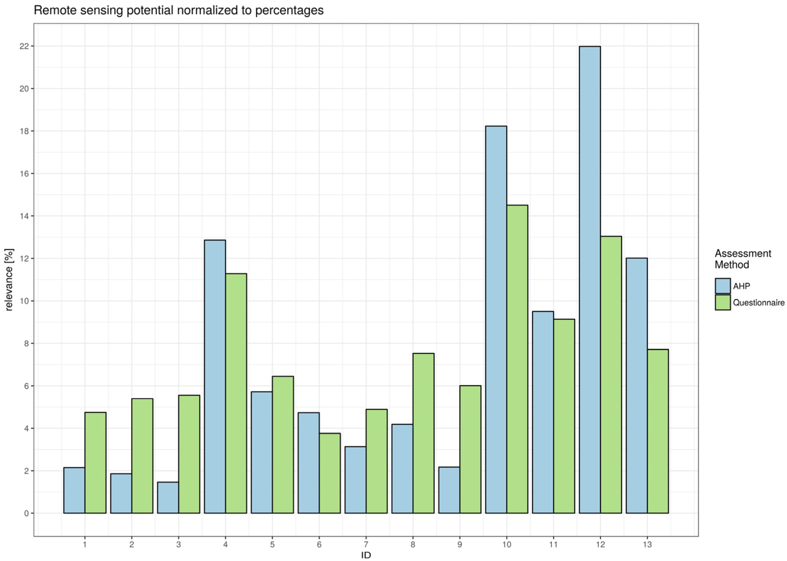
| ID | Indicators | Weights of Questionnaires | Weights of AHP Procedure |
|---|---|---|---|
| 1 | Energy consumption of public buildings per year (kWh/m2) | 4.75 | 2.09 |
| 2 | Total electrical energy use per capita (kWh/year) | 5.39 | 1.88 |
| 3 | Noise pollution | 5.55 | 1.47 |
| 4 | Square meters of public outdoor recreation space per capita | 11.28 | 12.72 |
| 5 | Percentage of city population living in slums | 6.44 | 5.78 |
| 6 | Percentage of households that exist without registered legal titles | 3.76 | 4.60 |
| 7 | Percentage of the city’s solid waste that is disposed of in a sanitary landfill | 4.89 | 3.28 |
| 8 | Kilometers of high capacity public transport system per 100,000 population | 7.53 | 4.16 |
| 9 | Number of personal automobiles per capita | 6.01 | 2.20 |
| 10 | Green area (hectares) per 100,000 population | 14.51 | 18.73 |
| 11 | Areal size of informal settlements as a per cent of the city area | 9.14 | 9.58 |
| 12 | Land area (square kilometers) | 13.04 | 21.82 |
| 13 | Percentage of non-residential area (square kilometers) | 7.71 | 11.70 |
| Indicators Provided by the Remote Sensing Experts | Adequate Equivalent Indicators Found in the ISO 37120 |
|---|---|
| Public transport capability (using street network/building blocks as proxy) |
|
| |
| Population density per km2 estimated by the size/heights of the buildings |
|
| Potential for solar energy on roofs within the city |
|
| 3D city models for sustainable planning of green/smarter cities | no matches found |
| Urban ventilation corridors (km2) |
|
| Water pollution |
|
| |
| Potential of building roofs to be used for solar energy production (roof’s area, aspect, slope, shading situation due to neighboring buildings, vegetation, terrain) |
|
| Population would be necessary for many parameters, land use/zoning would be useful | no matches found |
| Average height of construction | no matches found |
| Rank | Identified Indicators by Means of the Online Questionnaire Approach | Identified Indicators by Means of the Pairwise Comparison Approach (AHP) |
|---|---|---|
| 1 | Green area (hectares) per 100,000 population | Land area (square kilometers) |
| 2 | Land area (square kilometers) | Green area (hectares) per 100,000 population |
| 3 | Square meters of public outdoor recreation space per capita | Square meters of public outdoor recreation space per capita |
| Online Questionnaire Approach | Pairwise Comparison Approach (AHP) | |
|---|---|---|
| Advantages |
|
|
| Disadvantages |
|
|
© 2018 by the authors. Licensee MDPI, Basel, Switzerland. This article is an open access article distributed under the terms and conditions of the Creative Commons Attribution (CC BY) license (http://creativecommons.org/licenses/by/4.0/).
Share and Cite
Lehner, A.; Erlacher, C.; Schlögl, M.; Wegerer, J.; Blaschke, T.; Steinnocher, K. Can ISO-Defined Urban Sustainability Indicators Be Derived from Remote Sensing: An Expert Weighting Approach. Sustainability 2018, 10, 1268. https://doi.org/10.3390/su10041268
Lehner A, Erlacher C, Schlögl M, Wegerer J, Blaschke T, Steinnocher K. Can ISO-Defined Urban Sustainability Indicators Be Derived from Remote Sensing: An Expert Weighting Approach. Sustainability. 2018; 10(4):1268. https://doi.org/10.3390/su10041268
Chicago/Turabian StyleLehner, Arthur, Christoph Erlacher, Matthias Schlögl, Jacob Wegerer, Thomas Blaschke, and Klaus Steinnocher. 2018. "Can ISO-Defined Urban Sustainability Indicators Be Derived from Remote Sensing: An Expert Weighting Approach" Sustainability 10, no. 4: 1268. https://doi.org/10.3390/su10041268