Factors Causing Farmland Price-Value Distortion and Their Implications for Peri-Urban Growth Management

Abstract

Taiwan’s Agricultural Development Act (ADA) of 2000 relaxed farmland ownership criteria and allowed non-farmers to own farms. Although this opened up the market and induced a growth in farmland trading, relaxing these criteria without proper monitoring resulted in rapid development of farmhouses that fragmented farmlands, adversely affecting agricultural production and the quality of peri-urban environments, and increased management difficulties. Relaxing farmland ownership criteria also provided opportunities for speculation, which pushed up farmland prices, causing farmland price to deviate from its production value. We used a price:value ratio as an index of price-value distortion to explore farmland price-value distortion spatially using a geographical information system (GIS). Yilan County was used as a case study since its agricultural lands suffer high development pressure due to ready accessibility from the Taipei metropolitan area. Ordinary least square and quantile regression were used to identify factors driving distortion in Yilan County. Finally, we discuss the distortion and key factors for specific sites in Yilan to assess the urban sprawl and propose a preliminary course of action for peri-urban growth management. Our findings suggest that residential activities stimulate farmland price-value distortion but do not enhance farmland value. Designation of a land parcel as agricultural within an urban area allows for speculation and increases distortion. The land parcel’s association with infrastructure such as road and irrigation systems, and the price of agricultural products, are significantly correlated with distortion. Most of these identified factors increased farmland price because of the potential for non-agricultural land-use. We propose that to resolve farmland price-value distortion in Yilan, multi-functional values, in addition to agriculture, must be envisioned.

1. Introduction

A number of environmental impacts within farmlands and their surrounding areas are the result of current land-use planning and policies, which emphasize economic development over environmental protection, ecological conservation, and control of urban sprawl into farmlands [1,2]. Urban sprawl encompasses a complex pattern of land-use, transportation, and socioeconomic development [3], depending on the type of urban and rural planning and farmland policies [4]. Factories in rural areas, regarded as industrial land-use, are inextricably linked with urbanization and the urban sprawl pattern in Taiwan [5,6,7]. Moreover, urban sprawl into farmlands in Yilan shows a unique pattern due to the presence of farmhouses occurring both along roadsides and in the middle of farmlands, a result of amendments to the Agricultural Development Act (ADA) in 2000 that allowed for residential activities on farmland. The resultant pattern differs from the “Frog Jump” pattern observed in western countries. The urban sprawl developing along the roadside and in the middle of farmlands caused adverse impacts on the peri-urban environment and complicated sprawl management.

While agricultural production is the most conventional way of gaining revenue from farmlands currently, it is anticipated that there will be greater returns from farmlands through farmland readjustment in the future [8]. Urban sprawl onto farmlands in Yilan is a result of the comparative advantage of farmland owners and developers. The findings of Hardie et al. [9] suggested that in general, farmland and housing prices are determined by income, population, and accessibility variables. This implies that option values associated with irreversible and uncertain land development are capitalized into current farmland values. Plantinga et al. [8] decomposed farmland value into two components: (1) the quasi-rents from agricultural production and (2) the gains from potential land development at the nation’s county level. Kostov [10] applied spatial quantile regression and hedonic land price to model agricultural land sales in Northern Ireland. Later, McMillen [11] applied quantile regression to spatial grid modelling in the Chicago area and in this way predicted the change in land values as one moves closer to the central business district of the city. Yoo and Frederick [12] used quantile regression to statistically explore the effects of land subsidence and earth fissures to residential property values in a study from Arizona. Few studies, however, have concentrated on the spatial pattern of both farmland price and value and their distribution difference at site scale with geographical information system (GIS) spatial analyses.

Current farmland prices are mostly driven by the option values of potential development, which often surpass the land’s production value. Farmland prices are thus frequently higher than would be expected from their production value. With a lack of proper monitoring, speculators entered the farmland market, and a scattering of farmhouses emerged on the Yilan Plain. The agricultural production zone and surrounding areas continue to suffer from an array of environmental impacts caused by the increase of residential housing and over-development that occurred once the ADA was amended. Therefore, current farmland prices, representing the option values of potential farmland development, are a paradoxical excuse for farmland speculation in Taiwan. Because the agricultural development policy no longer stipulated that farmland had to be utilized for agricultural production and allowed development of residential buildings on farmlands, building companies and land owners triggered speculation of real estate on farmland. This caused a substantial farmland price increase and thereby distorted its price-value ratio. In Yilan, the price-value distortion of farmlands resulted in decreased agricultural production and affected farmland ecosystem services.

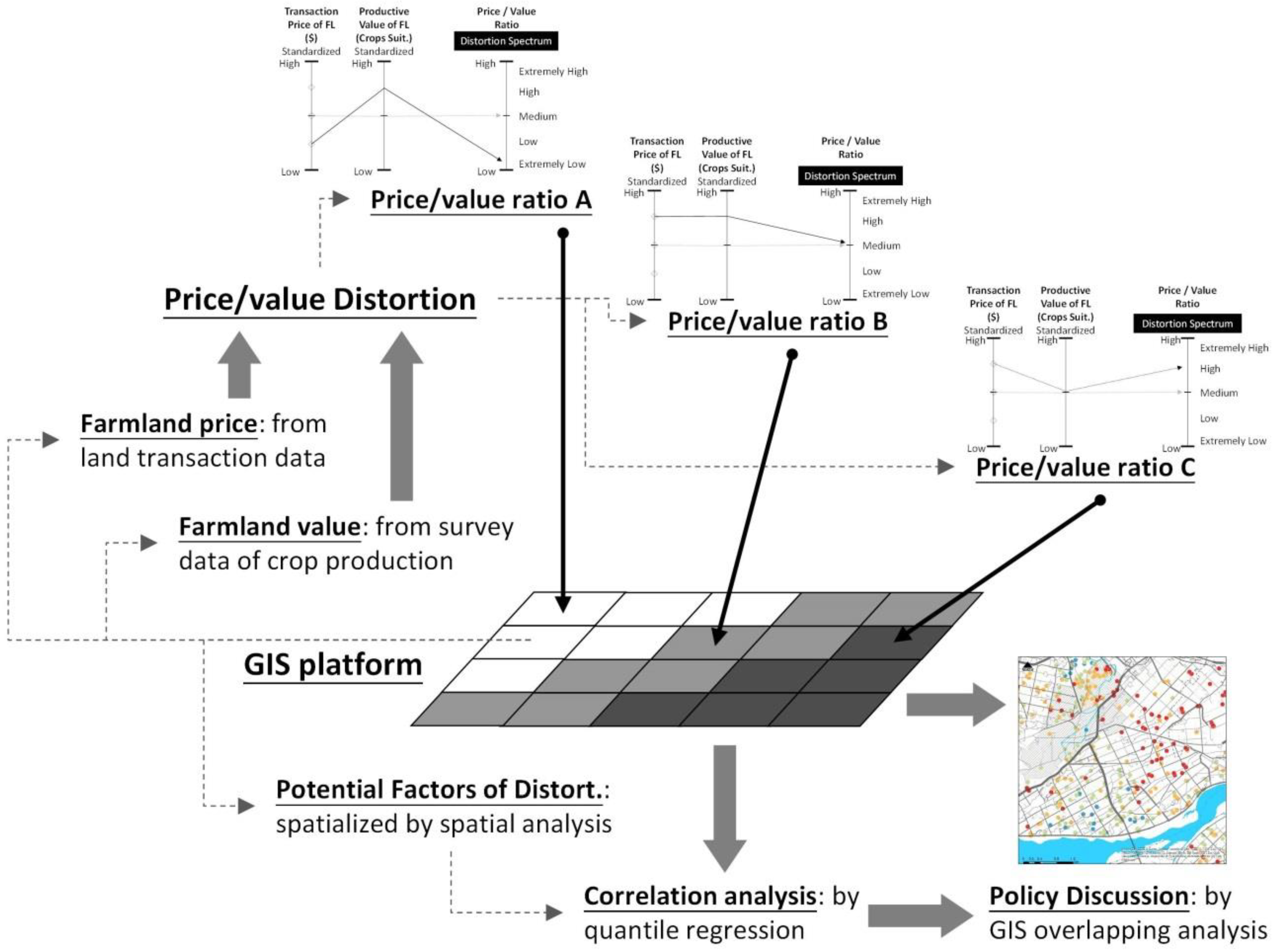
We used Yilan County as a case study to investigate spatial patterns of this price-value distortion. We used a GIS platform to integrate a farmland transaction database (price) with the value of crop production (using a “relative value from production” approach). A quantile regression (QR) was used to identify factors potentially impacting the price-value distortion for each farmland transaction. These factors were explored with spatial analyses to review the spatial pattern of the distortion relative to planning and management policies. This was used to propose potential measures to manage the price-value distortion and enhance ecosystem services of farmlands in Yilan.

2. Research Background

2.1. Farmland and Farmhouse Development in Yilan

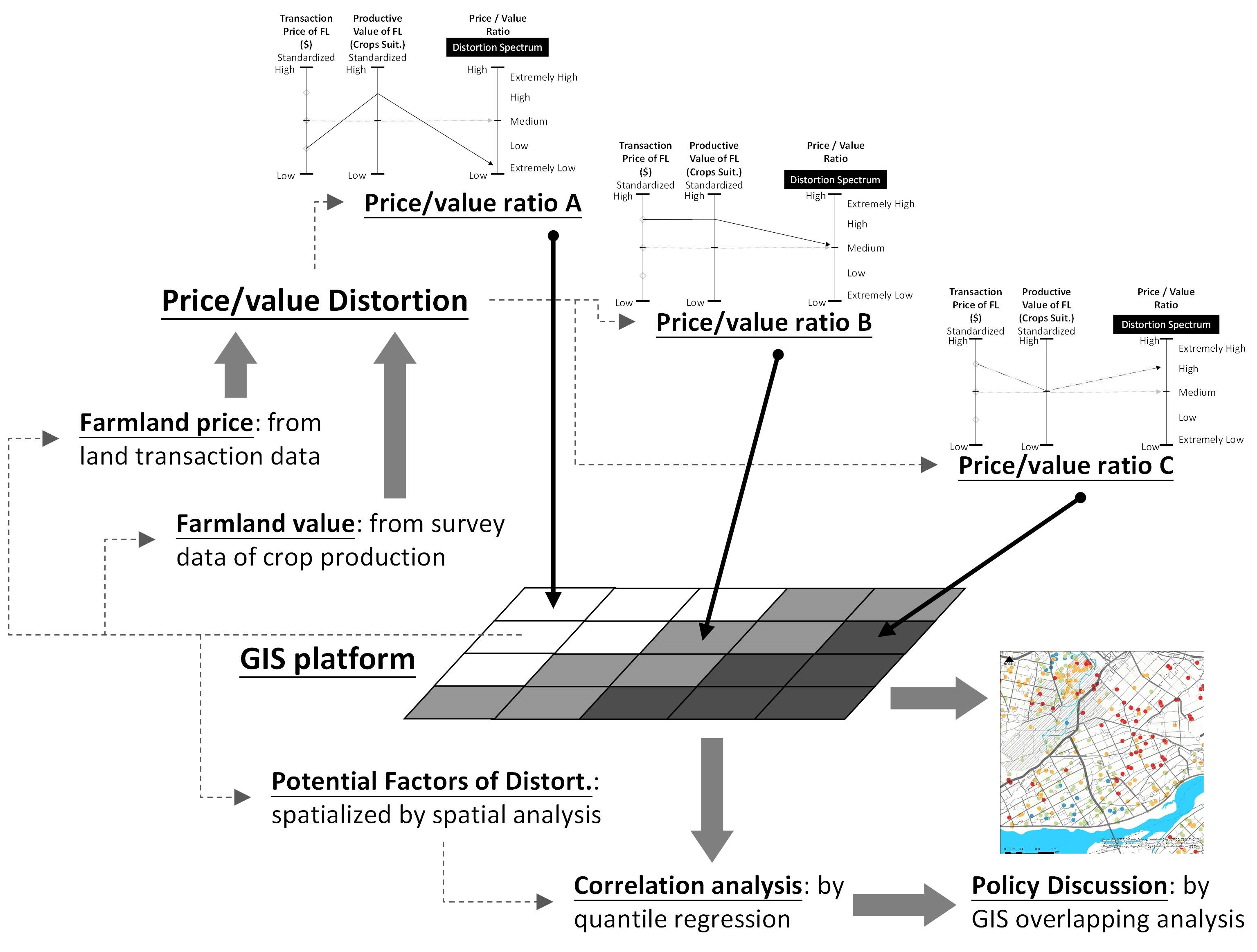
Yilan County, located in the northeast of Taiwan, is adjacent to the Taipei metropolitan area (Figure 1). It has an area of 2144 km². 14.93% of the land is a plain, known as Lanyang Plain (24°37′–24°50′ N, 121°37′–121°50′ E). Its soil quality, sufficient precipitation, and efficient irrigation system make it an important agricultural production region in Taiwan. After Taiwan’s Agricultural Development Act revised farmland ownership criteria to allow non-farmers to own farmlands in 2000, many urban civilians became farm owners and are now hobby farmers or simply build farmhouses in the production area. The completion of National Freeway No. 5 in 2006 shortened travel time, and commuting between Yilan County and Taipei city became feasible. This provided further incentives for urban residents to pursue agri-tourism in Yilan, or even to purchase farmland there. These factors all increased the transformation of Yilan from a conventional farming area into an agri-tourism industry. As a result, a large number of farmhouses were built on farmlands which caused a rapid urban sprawl pattern on the Lanyang Plain, hindering production as well as the development of agricultural industries in Yilan County [13].

To mitigate the problem, the “Regulations for Constructing Farmhouses on Agricultural Land in Yilan” (hereafter “Farmhouse Regulations”) were implemented by the Yilan County Government in 1994. They provided guidance for building farmhouses that suited the landscape and environment. Subsidies were offered for compliance, which attracted speculators and led to more farmhouses appearing on the Lanyang Plain. The demand for farmland was strong, and elevated farmland prices and a unique pattern of urban sprawl emerged on the Lanyang Plain. As Huang [14] pointed out, when it is anticipated that farmland prices will be inflated in the future, speculation prevails. This is exactly what occurred in Yilan County. It is important to realize that once farmland has been converted into buildings, both cultivation area and agricultural production value are decreased, and farmland ecosystem services, which are socioeconomically and environmentally important, will suffer from the loss of farmland [15].

2.2. Farmland Price and Value

When only farmers owned farmland, agricultural production was the most common source of revenue. As a result, farmland value was determined based on the output level or profitability of agricultural production, and transaction prices of farmland usually reflected its production value [16], implying little deviation between farmland price and value. Since the criteria for farmland ownership were relaxed and farmland policy shifted from “farmland should be owned by farmers” to “farmland should be used for agricultural production”, non-farmers have been allowed to own farmland. This caused a loophole allowing for speculation. It is anticipated that farmland readjustment (consolidation) will generate high returns and that farmland price will begin to deviate from its original purpose (i.e., production [8]). Rather than agricultural production value, the development potential of farmlands will play a vital role in determining farmland value and price. Hardie et al. [9] suggested that income, population, and other variables determine average farmland and housing prices. Their research suggests that optional values associated with irreversible and uncertain land development are capitalized into present farmland values.

The value and benefits of farmlands are worth assessing from a conservation and ecosystem services perspective. The multi-functionality of farmlands in providing such benefits as production value [16], water retention [17], wildlife habitats [18], air quality improvement [19], recreational and landscape aesthetics [20], and ecosystem services [21] has been the subject of many studies. However, this multi-functionality is based on the premise that farmlands are utilized for agricultural production rather than speculation. The capital gain from the potential development of farmlands cannot be combined with production value and other ecosystem services. Although taking ecosystem services into policy consideration is important, due to the difficulties of evaluating the value of ecosystem services of farmlands, its impacts on farmland price are not included in this study. Farmland prices in the following study therefore reflect the expected value of potential development (i.e., the possibility of building farmhouses) and agricultural production value. Discrepancies between farmland production value and farmland prices can be treated as proxies of “distortion”. Few studies have investigated the difference between prices and production values of farmlands, without which it is impossible to assess the significance of the role played by speculation.

3. Research Design and Data

3.1. Definition

Most previous studies have focused on factors influencing the price of farmlands, such as soil condition, production environment, and farmland productivity [22,23,24]. Since the advent of urbanization, additional factors have begun to influence land value. Arbitrage that hopes for appreciation may play a vital role in price decision. Therefore, analyzing the deviation between land price and its production value is helpful in understanding the current situation of farmland price distortion. The ratio of farmland price to farmland production value adjusted for the farmland price index, as defined in the present and earlier studies, reflects the level of distortion as follows:

$$\mathrm{price}-\mathrm{value}\mathrm{distortion}=\frac{\mathrm{price}\mathrm{of}\mathrm{farmland}}{\mathrm{value}\mathrm{of}\mathrm{farmland}}\times \mathrm{farmland}\mathrm{price}\mathrm{index}$$

The higher the ratio, the greater the distortion; a high distortion indicates a considerable discrepancy between farmland price and production value. Farmland price data were downloaded and summarized from the real estate transaction database provided by the Ministry of Internal Affairs. Farmland value was generated from the raw data of Taiwan’s agricultural census in 2010. Farmland price indices were collected from the Platform of Real Estate Information from the Ministry of Internal Affairs.

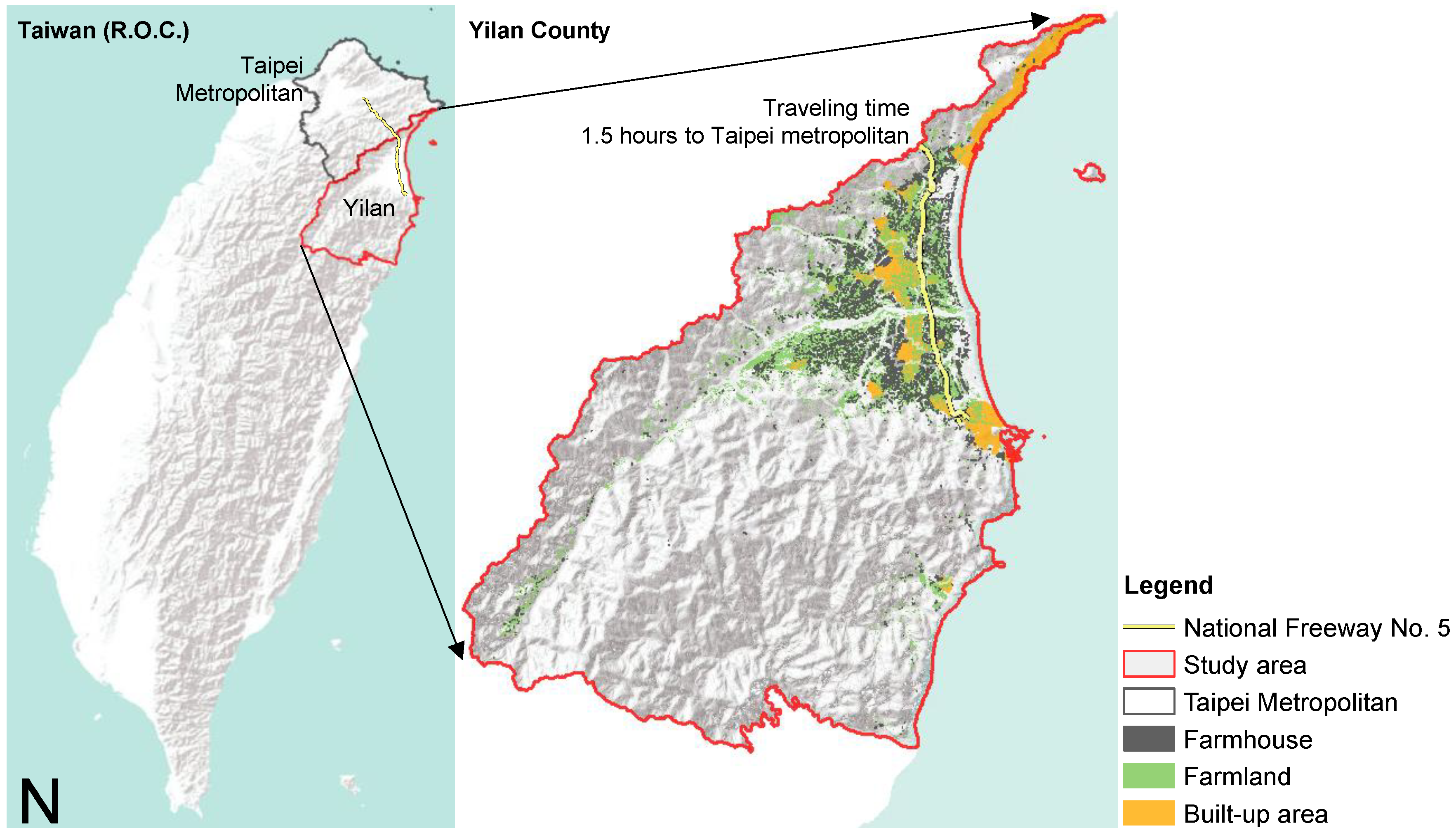
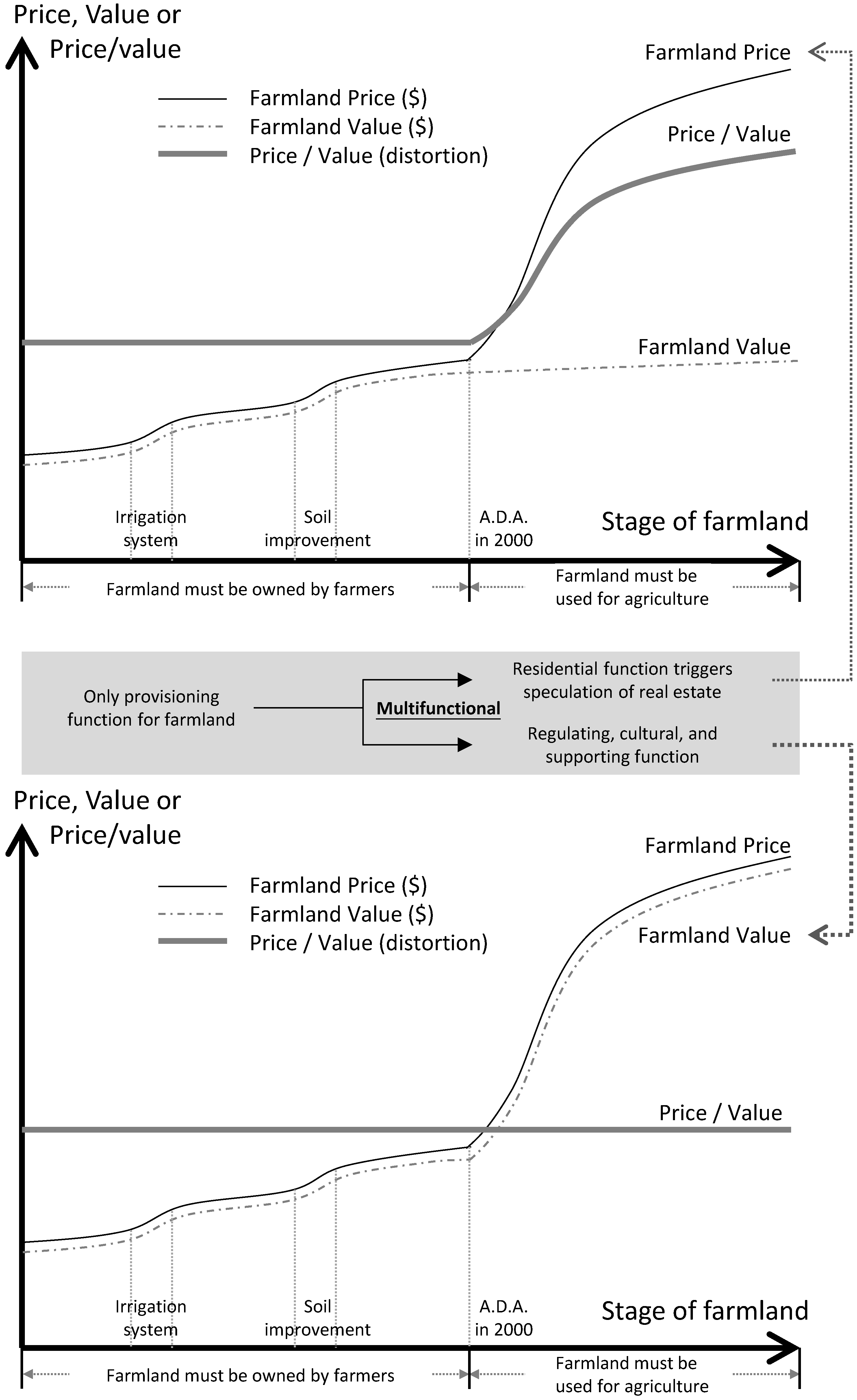
Before 2000, most Yilan farmlands were utilized for agricultural production because of the limitations of the ADA and zoning control for agricultural areas (Figure 2). During this period, farmland value was usually influenced by agricultural production and transportation cost from the perspective of land economics and location theory. Enhancing production conditions by irrigation system and soil improvement are examples of key methods for increasing farmland value and price. In this period, there was no obvious difference between farmland price and value. The farmland price increased substantially after the amendments of the ADA. Since farmland production value did not change, the farmland price:value ratio increased, resulting in a clear upward trend of price-value distortion. Subsequent studies revealed that farmland buildings along roads usually dominate the unique urban sprawl pattern in the surrounding environment of urban areas.

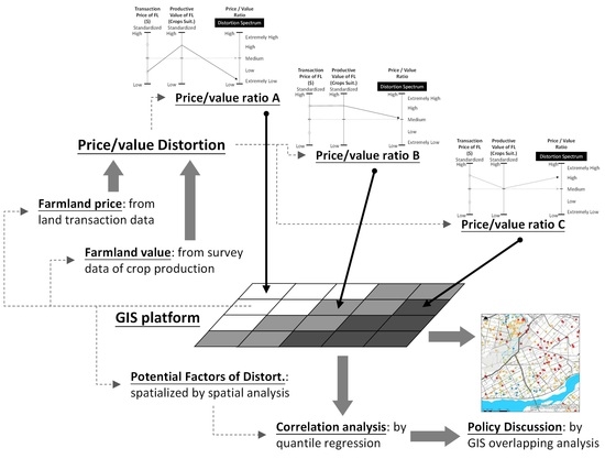
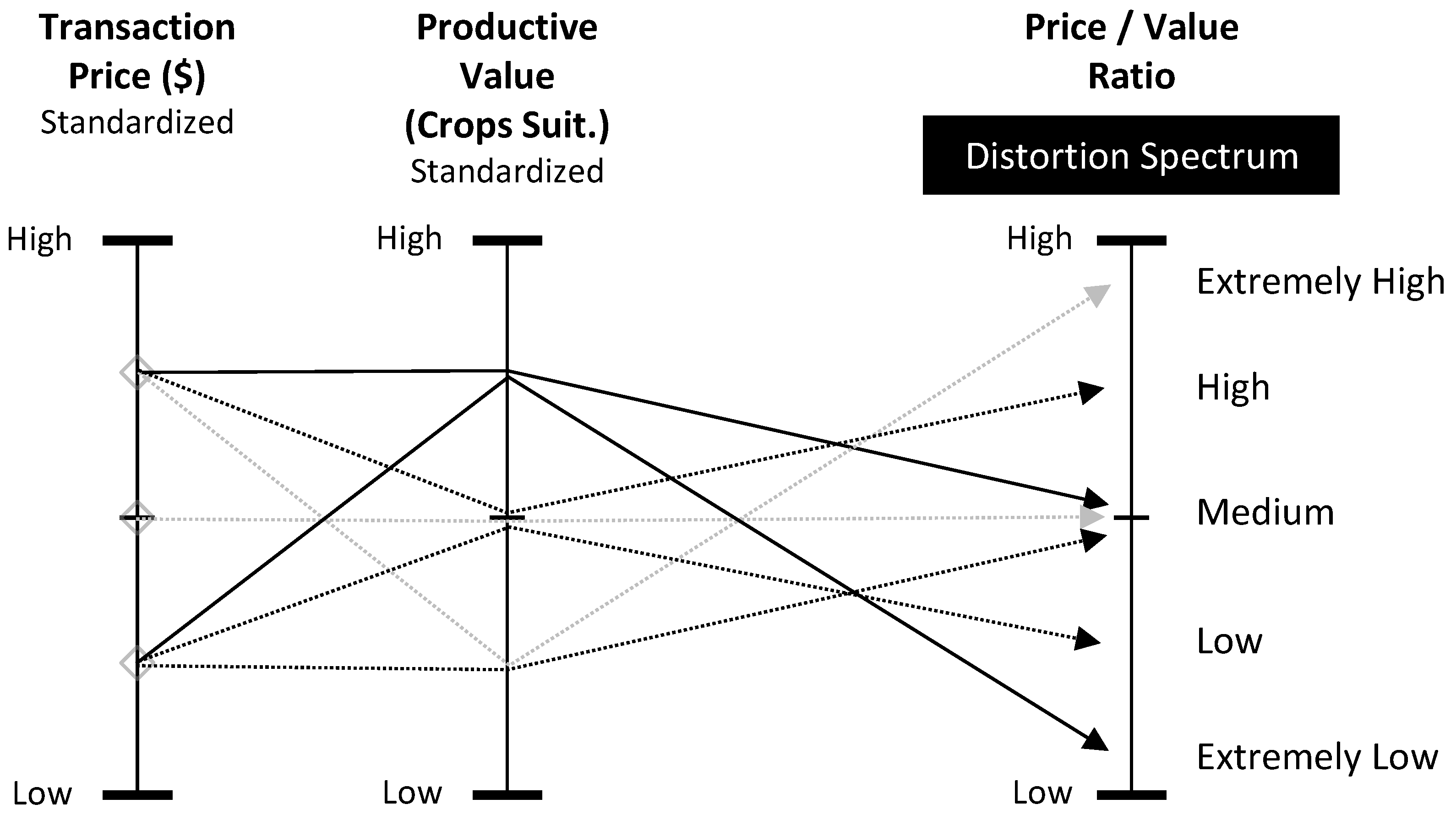
We adopt the price:value ratio firstly to generate a single index to analyze the phenomenon of farmland price-value distortion, and secondly to organize various scenarios for analyzing development impacts on good quality farmland. We then use this to discuss potential issues arising from farmland protection and demand for urban development (Figure 3). For example, farmland with both a high transaction price and a high productive value is identified as a good quality farmland in Yilan. Its price:value ratio (price-value distortion) is usually a result of serious urban development impact. Therefore, besides distortion, relative and standardized measures based on crop production value and farmland price as determined from land transactions were also used to explore farmland value. The farmland price:value ratio shows an interesting distortion spectrum which highlights the conflict between land speculation, farmland preservation, and urban growth management.

3.2. Research Design

A geographical information system (GIS) was used to integrate farmland transaction, to spatially illustrate the distortion spectrum (Figure 4), and to identify and estimate potential factors influencing the distortion. Quantile regression (QR) was also adopted to estimate the impact of factors on the distortion. The spatial pattern of the distortion relative to planning and management policies and their implications were discussed as well. Suggestions were provided to manage distortion, preservation, and urban growth management in Yilan.

3.3. Data

We selected eight potential factors influencing farmland price and production value: soil condition (a proxy for crop suitability); irrigation system; crop price variation; farmland use regulation; distance of farmland from urban area; width of the nearest road; complexity of land count and transaction; and real estate loan index [13,22,23,24,25,26,27,28]. Calculating farmland price and value in this study focuses on farmland itself without considering the price of farmhouses. In addition to calculating distortion and these factors (

Table 1. The definitions and sources of variables.

Variable	Definition and Data Description	Data Source
Price	Real transaction price of farmland (NT$/m2) (transaction price of farmland from 2012 to 2015 is adjusted by consumer price index to have a common comparative base in 2016)	Actual real estate transaction cases, Ministry of the Interior (August 2012–September 2016)
Value	Production value of farmland (NT$/m2/year) (average production value of crops per year is calculated from the original database based on the location for each farmland transaction)	Agricultural, Forestry, Fishery and Husbandry Census, Directorate General of Budget, Accounting and Statistics (2016)
Price_value	Price-value distortion (ratio of the real transaction price to production value, %)	(Same as above)
Avgattr	Soil conditions (0 is the poorest, 4 is the best)	NGIS Ecological Resources Database
near_water	Distance to the nearest canal (m)	Platform for the National Land Use Inventory
Agriprice	Annual crop prices variation (%)	Statistical database of Yilan County; Agricultural Statistics Yearbook, Council of Agriculture
use_urban	Agricultural zone in urban area (1 yes, 0 no)	Actual information of real estate transaction case, Ministry of the Interior
use_regular	General agricultural zone in non-urban area? (1 yes, 0 no)	(Same as above)
use_special	Special agricultural zone in non-urban area? (1 yes, 0 no)	(Same as above)
use_mt	Sloping and conservation zone in non-urban area? (1 yes, 0 no)	(Same as above)
near_urban	Distance to the nearest urban area (m)	Layers of use in urban planning, Construction and Planning Agency, Ministry of the Interior
Width	The width of the nearest road (m)	Taiwan Electronic Map, Ministry of the Interior
Landcount	Complexity of land counts (1, 2, 3, etc.) (many approaches could be used to define complexity of land. To simplify the problem, as well as to cope with the real situation of Yilan, the complexity of farmland ownership was applied in this research instead of common landscape metrics, Shannon index, or landscape complexity [29].)	Agricultural cadastral maps, Yilan County
Interestrate	Mortgage rate (%)	Deposit and loan rate of five leading domestic banks, Central Bank

and

Table 2. Descriptive statistics of variables.

Variable	Mean	SD	Maximum	Minimum
Price_value	306.14	360.11	5223.48	0.19
Avgattr	3.16	1.27	4	0
near_water	258.94	507.44	4921.98	0
Agriprice	2.73	7.22	29.84	−50.34
use_urban	0.08	0.28	1	0
use_regular	0.16	0.37	1	0
use_special	0.68	0.47	1	0
use_mt	0.08	0.27	1	0
near_urban	2047.44	2200.73	38,770.77	0
Width	5.77	3.24	40	1
Landcount	8.74	6.66	75	1
Interestrate	1.37	0.04	1.38	1.12

), QR and ESRI ArcGIS were used to analyze the farmland price determination in Yilan County. Our findings indicate that the factors (or explained variables) do affect distortion.

3.4. Results

3.4.1. Illustration of Price-Value Distortion in Yilan County

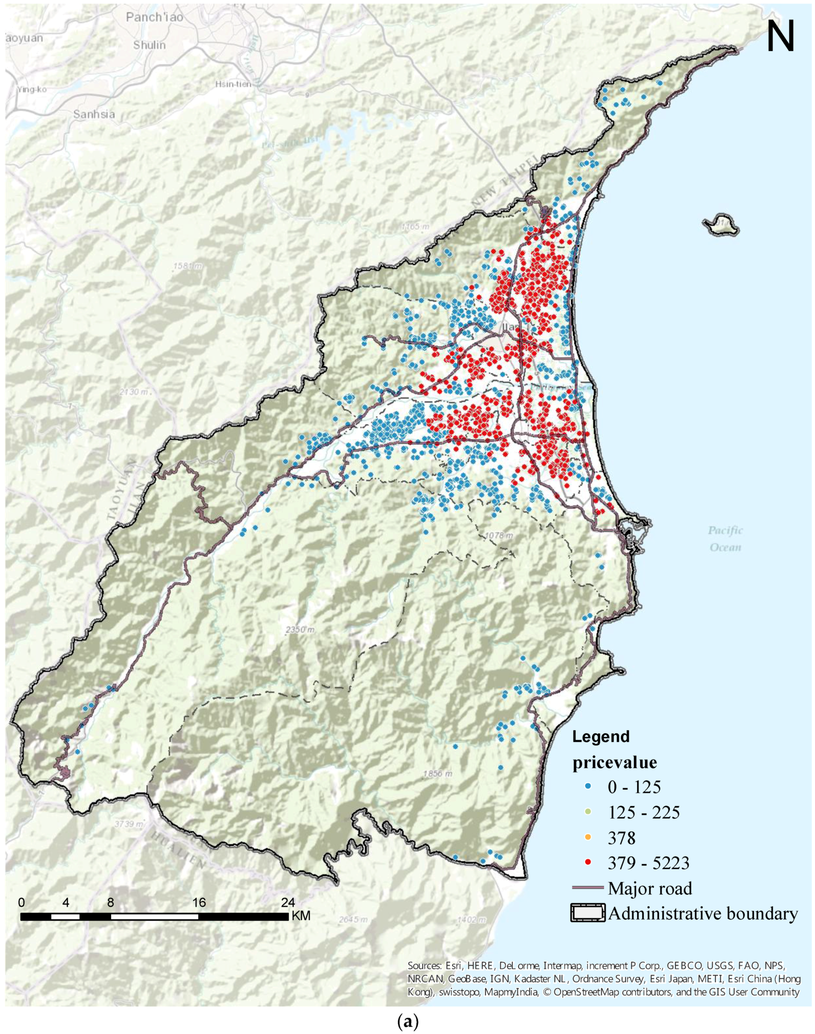
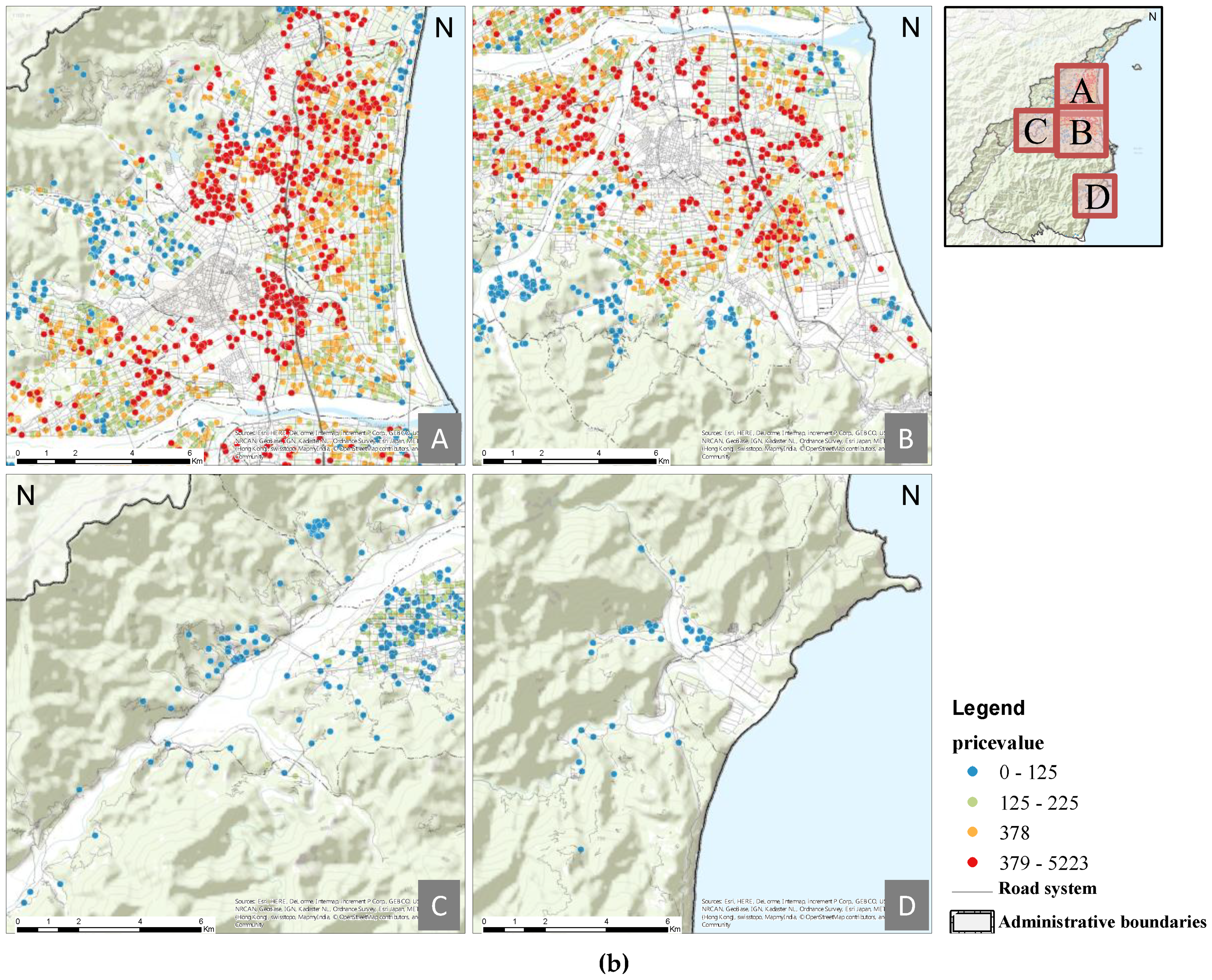
The categories of distortion, from low to high, are shown as blue, green, orange, and red (Figure 5). To facilitate comprehension, quartiles were used to define the bounds of each distortion category. The calculated distortion categories of Yilan County indicate that areas in the plain were the most heavily traded. Among these, areas with a high density of high distortion instances were Yilan City (Figure 5(b),A), Luodong Township (Figure 5(b),B), Zhuangwei Township, Wujie Township, Dongshan Township, and Jiaosi Township. Transactions decreased with distance from the city or towns (as illustrated by the color distribution of the symbols changing from orange to green and then to blue in Figure 5). Figure 5 shows that these areas are east of Yuanshan Township, Sansing Township, Datong Township (Figure 5(b),C), and Nan’ao Township (Figure 5(b),D).

3.4.2. Ordinary Least Square (OLS) Regression and Quantile Regression (QR) Analyses for Price-Value Distortion of Farmlands in Yilan County

In addition to visualizing distortion by area with ArcGIS, quantitative analysis was used to examine the factors influencing distortion. In an ordinary least square regression model, the calculated distortion was treated as the dependent variable, and suitability for crop plantation, the distance to the nearest canal, crop price variation, land usage regulation, distance to the nearest urban planning areas, width of the nearest road, the complexity of land counts, and mortgage rates were treated as explanatory (independent) variables. The full regression model can be expressed as:

$$\begin{array}{l}{\mathrm{price}\text{\_}\mathrm{value}}_{\mathrm{i}}=\\ {\mathsf{\beta }}_0+{\mathsf{\beta }}_1\mathrm{avgattr}+{\mathsf{\beta }}_2\mathrm{near}\text{\_}\mathrm{water}+{\mathsf{\beta }}_3\mathrm{agriprice}+{\mathsf{\beta }}_4\mathrm{use}\text{\_}\mathrm{urban}+{\mathsf{\beta }}_5\mathrm{use}\text{\_}\mathrm{special}+{\mathsf{\beta }}_6\mathrm{use}\text{\_}\mathrm{mt}\\ +{\mathsf{\beta }}_7\mathrm{near}\text{\_}\mathrm{urban}+{\mathsf{\beta }}_8\mathrm{width}+{\mathsf{\beta }}_9\mathrm{landcount}+{\mathsf{\beta }}_{10}\mathrm{interestrate}+{\mathsf{\epsilon }}_{\mathrm{i}},\mathrm{i}=1,2,3,\text{…},4641\end{array}$$

The results of the OLS model are shown in

Table 3. OLS (ordinary least square) and QR (quantile regression) results for the price-value distortion of farmland in Yilan County.

Variable	OLS	QR (θ)
		0.1	0.25	0.5	0.75	0.9
constant	430.334 ***	10.264 **	119.658 *	266.637 ***	249.612	1291.145 ***
	(3.02)	(3.11)	(1.88)	(3.13)	(1.29)	(3.31)
avgattr	2.196	1.807	0.736	4.619 *	15.066 ***	17.748
	(0.43)	(1.38)	(0.46)	(1.73)	(3.98)	(1.47)
near_water	−0.0284 **	−0.004	−0.012 ***	−0.018 ***	−0.017 ***	−0.017 *
	(−2.33)	(−1.44)	(−3.50)	(−4.17)	(−3.79)	(−1.73)
agriprice	1.779 ***	0.125	0.577 ***	1.080 ***	1.170 ***	1.719
	(2.79)	(0.87)	(2.1)	(3.81)	(2.54)	(1.45)
use_urban	600.541 ***	176.976 ***	298.907 ***	382.246 ***	690.964 ***	1335.272 ***
	(29.82)	(4.20)	(18.49)	(12.20)	(9.47)	(16.13)
use_special	82.934 **	63.083 ***	79.733 ***	92.831 ***	120.048 ***	117.442 ***
	(6.34)	(18.25)	(16.82)	(14.00)	(13.54)	(3.57)
use_mt	−64.989 **	−23.172 ***	−48.019 ***	−77.340 ***	−84.817 ***	−157.409 ***
	(−2.37)	(−4.52)	(−7.48)	(−7.55)	(−4.91)	(−3.33)
near_urban	−0.011 ***	−0.001	−0.000107	−0.002 *	−0.005 **	−0.007
	(−4.33)	(−1.30)	(−0.02)	(−1.56)	(−2.03)	(−1.34)
Width	17.831 ***	2.900 ***	4.733 ***	7.828 ***	15.472 ***	22.099 ***
	(12.62)	(3.31)	(6.38)	(6.76)	(7.12)	(5.00)
landcount	1.243 *	−0.329	0.299	1.173 **	3.271 ***	2.968 ***
	(1.84)	(−1.46)	(1.15)	(2.39)	(3.51)	(2.84)
interestrate	−235.224 **	−71.725 **	−54.222	−130.992 *	−111.256	−784.926 ***
	(−2.28)	(−2.44)	(−1.18)	(−2.17)	(−0.81)	(−2.81)
Adj./Pseudo R−Squared	0.283	0.1674	0.1664	0.1652	0.1902	0.2658
F statistic	183.99 ***
VIF	1.57

Note: 1. n = 4641; * p < 0.10, ** p < 0.05, *** p < 0.01. 2. The variance inflation factor (VIF) is used as an indicator of multicollinearity.

. All factors except for land count complexity significantly affected price distortion.

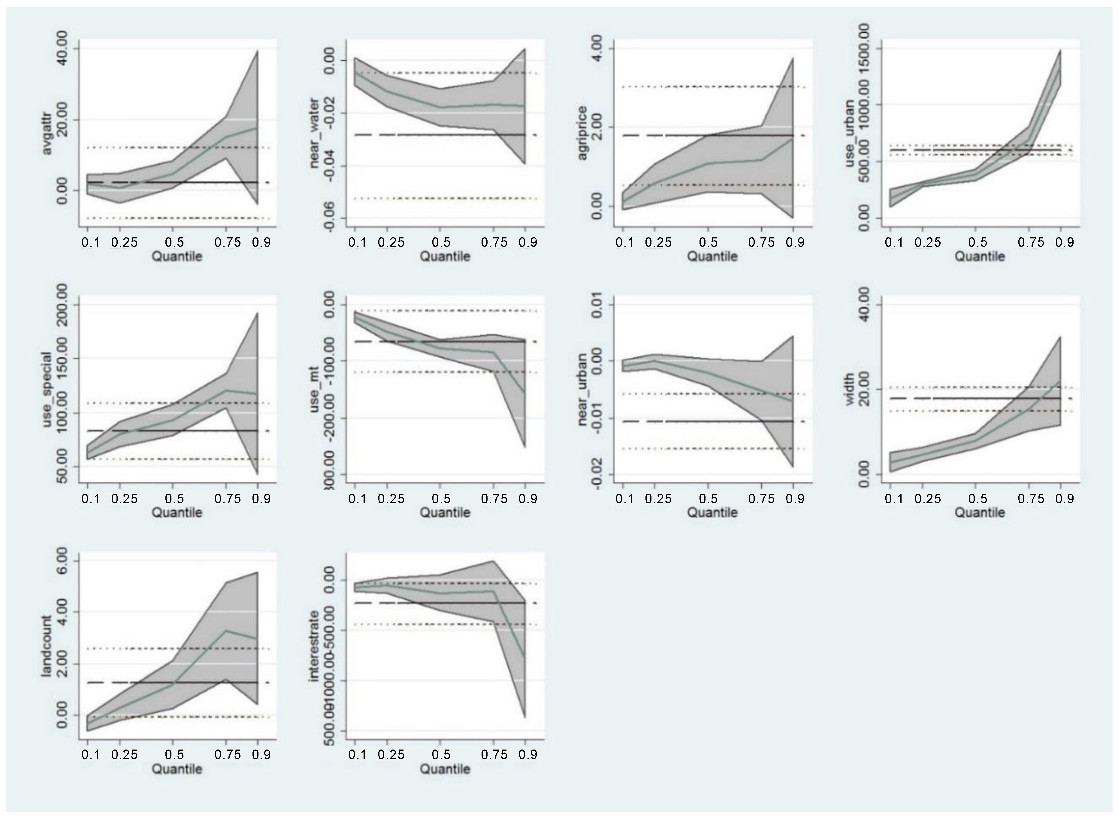
We also applied quantile regression, an approach initially introduced by Koenker and Bassett [30]. The model is used to examine the dynamic movement in each quantile and its main concept focuses on minimizing an asymmetrically weighted sum of absolute errors [31]. The relationships between dependent and independent variables under various circumstances at each quantile were discussed. In comparison to OLS models, a QR model can process samples with a non-normal distribution. Furthermore, the QR model was used to overcome a sample selection bias and outlier problems that were encountered when running the OLS model [31]. To conduct the QR, five quantiles (θ = 0.1, 0.25, 0.5, 0.75, 0.9) were used in our analysis to evaluate the impact of each factor on different distortion categories. The results (Table 3) show that the nearest distance to the canal, crop price variation, land use regulation, width of the nearest road, and the complexity of land count have positive impacts on distortion. The higher θ, the greater the distortion and when θ is higher, the impact of factors influencing distortion are higher. The confidence intervals calculated from the results of the OLS and QR are shown in Figure 6.

1. Distance to the main canal

The results suggest that distance to the nearest canal has a significant negative impact on distortion, with p < 0.01 in the 0.25, 0.5, and 0.75 quantiles, and p < 0.1 in the 0.9 quantile. Our findings suggest that when the farmland is separated by 1 m from the nearest canal, the distortion is reduced by 0.012%, 0.018%, and 0.017%, for the 0.25, 0.5, and 0.75 quantiles, respectively.

2. Crop price variation

Crop price variation has significant impact on distortion with p < 0.01 in the 0.25, 0.5, and 0.75 quantiles. Higher crop price variation is associated with greater distortion. The model indicates that when crop price variation increases by 1%, the distortion will increase by 0.577%, 1.080%, and 1.170% for the 0.25, 0.5, and 0.75 quantiles, respectively.

3. Land-use regulation

Land-use regulation has a significant impact on the price distortion with p < 0.01 under various quantiles. The price-value distortion is higher when the farmland is located in urban areas. In addition, the higher the quantile, the greater the distortion when farmlands are located in urban regions. The distortion is lower when the farmlands are located on slopes or conservation fields in non-urban zones. Compared to urban areas, distortion decreased at higher quantiles in non-urban zones.

4. Width of the nearest road

Width of the nearest road significantly affects price-value distortion under various quantiles. When the width of the nearest road widens by 1 m, the distortion is increased by 2.900%, 4.733%, 7.828%, 15.472%, and 22.099% for the 0.1, 0.25, 0.5, 0.75, and 0.9 quantiles, respectively. This suggests that the higher the quantile, the greater the impact of road width on distortion.

5. Complexity of land count

The complexity of land count significantly affects farmland distortion with p < 0.01 in the 0.5 and 0.9 quantiles. This implies that an increase in the number of farmland transactions in buffer areas causes distortion to increase by 1.173%, 3.271%, and 2.968% in the 0.5, 0.75 and 0.9 quantiles, respectively. If the quantile is less than or equal to 0.75, higher complexity of land count results in a greater distortion. The distortion reached its peak in the 0.75 quantile.

4. Discussion

4.1. Designating an Urban Area Tends to Increase the Price-Value Distortion of Agriculture Zones

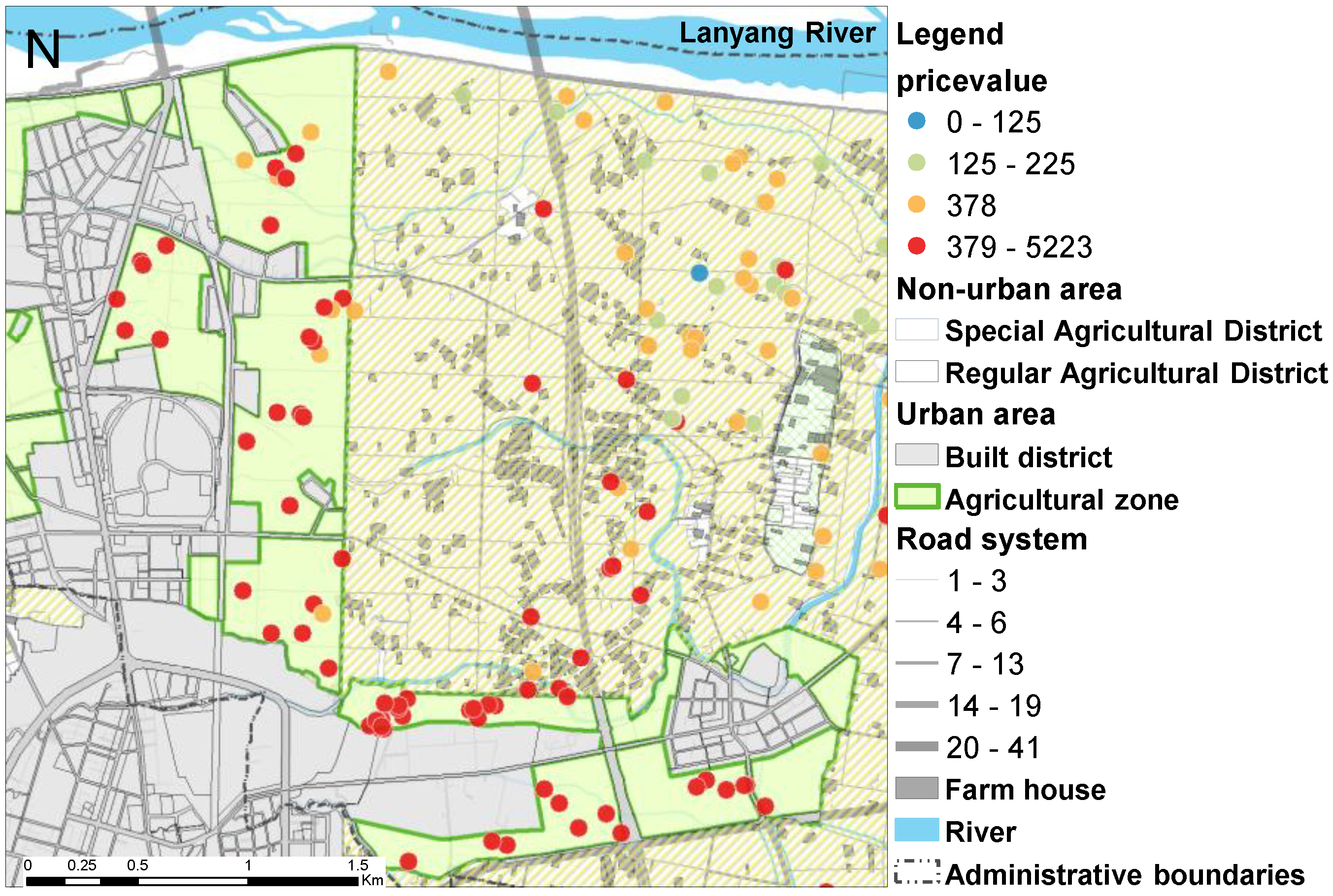
Few of Taiwan’s urban plans have been designed from the perspective of agricultural development or the multi-functionality of agriculture. These plans often imply that farmlands located in urban areas will eventually be developed for non-agricultural use. Farmlands located in urban areas are targets for speculation (Figure 7). Due to the anticipated capital gain, the prices of these farmlands are increasing, which will hinder development in these areas. It will also increase the price-value distortion ratio. Therefore, designating urban zoning in agricultural zones tends to increase the price-value distortion of farmlands.

4.2. A Better Road or Transportation System in Agricultural Zones Tends to Increase the Price-Value Distortion

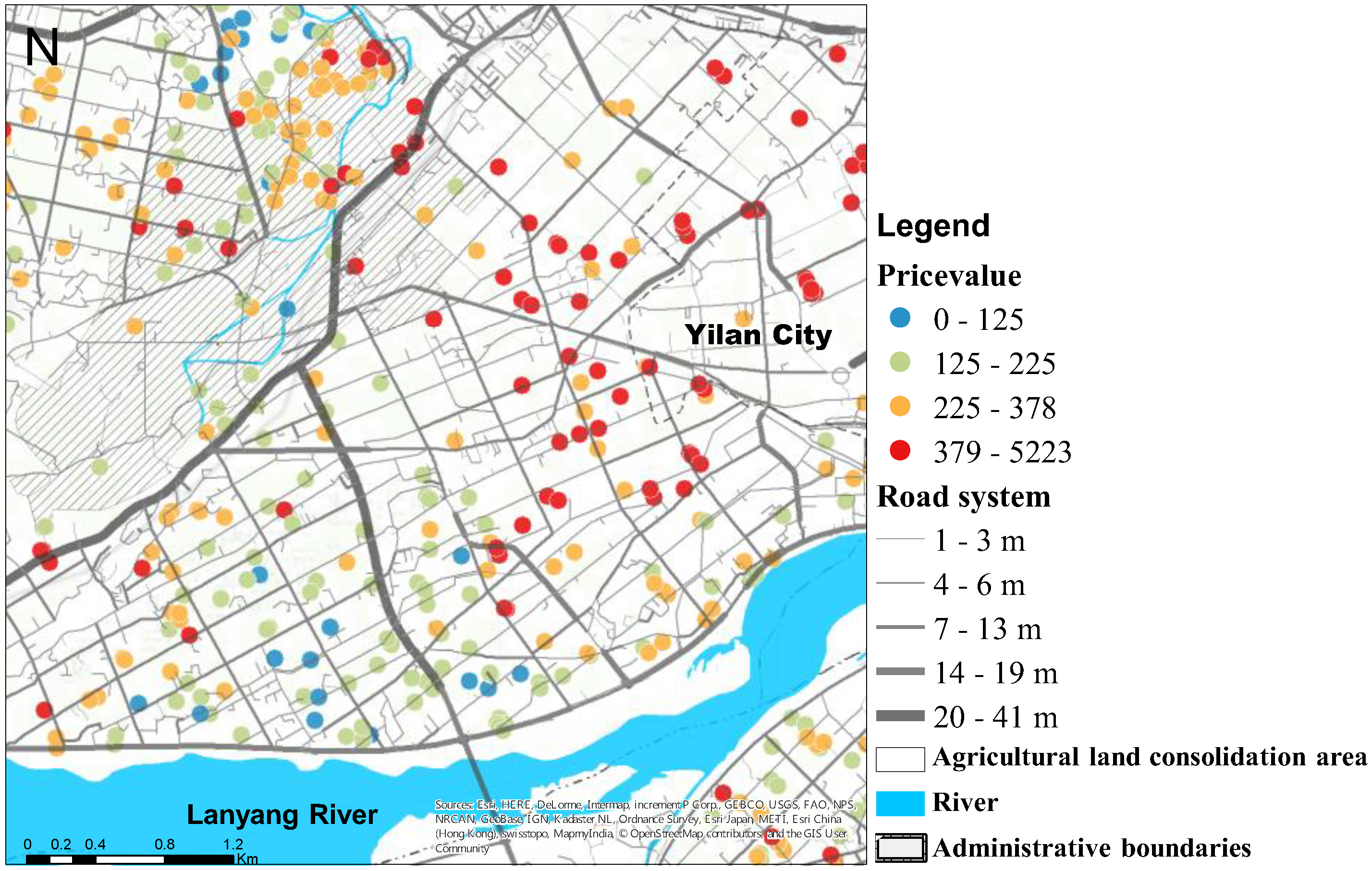
Road or transportation system accessibility is important for agricultural marketing. The width of roads is often regarded as an indicator of transportation conditions. Under the Building Act of Yilan County, the width of the nearest road was set as a minimum requirement for constructing farmhouses. A better road system therefore tends to elevate the price of farmlands. Our model suggests that road condition is highly correlated with price-value distortion, and this is consistent with reality. Figure 8 illustrates clusters of high distortion that correspond to the pattern of road width in Yuanshan Town.

4.3. Farmland Reform Policy Significantly Affects Price-Value Distortion

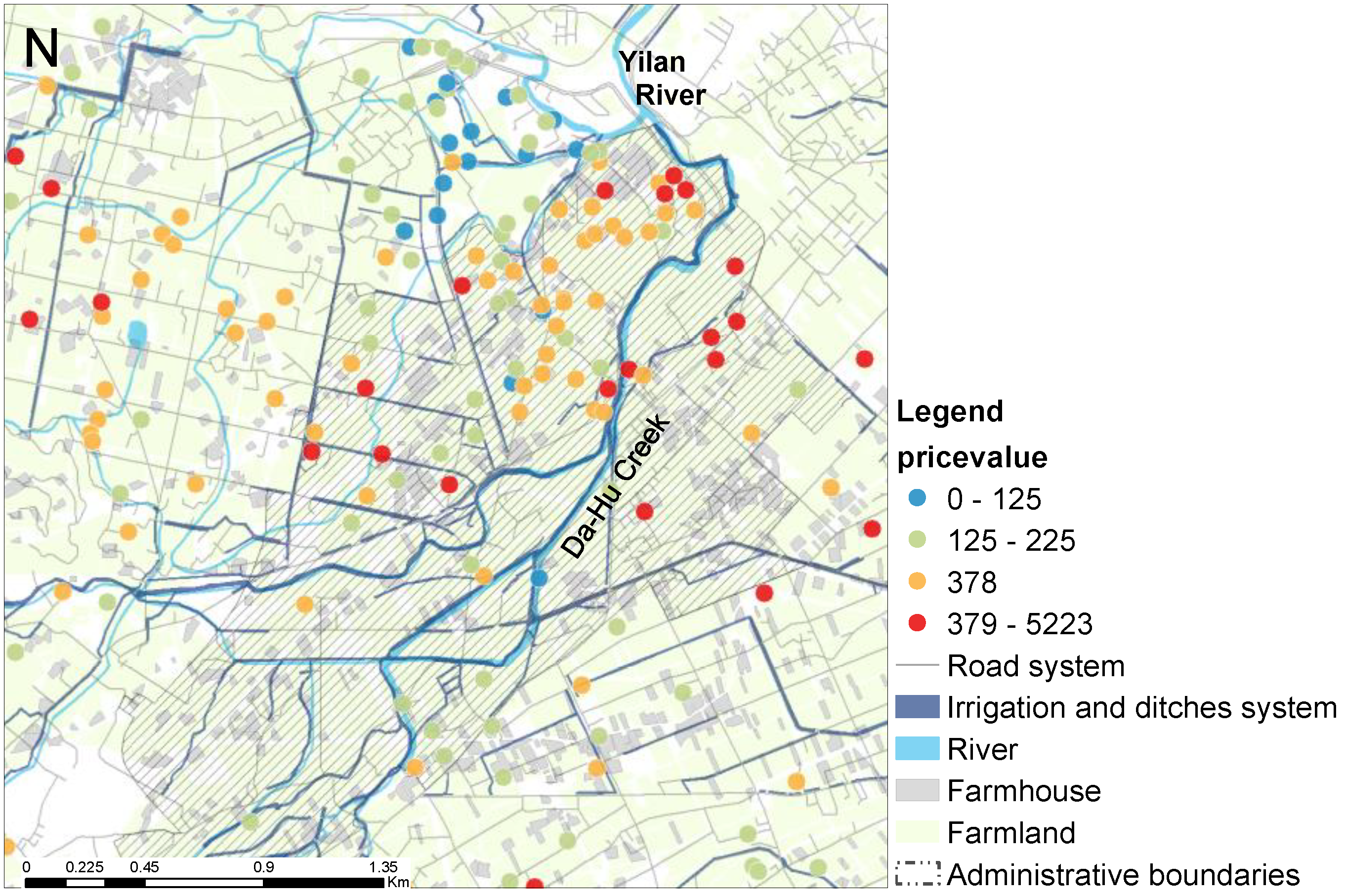
Farmland readjustment is one of the major policy mechanisms for improving the productivity of agriculture. The process aims to produce ordered farmland parcels suitable for mechanization and better irrigation systems. A better agricultural production environment increases land price but enhances the possibility of higher distortion. The regression analysis outcomes suggest that there is an important relationship between distortion and distance between farmlands and irrigation systems in Yilan. Figure 9 shows that in Yuanshan Town, higher distortion occurs in areas with better irrigation systems developed through the farmland readjustment plan. The Agricultural Development Act amendments in force since 2000 shifted the policy goal from “farmland owned by farmers” to “farmland used for agriculture”. This policy relaxed the criteria for ownership of farmland, which positively affected farmland price, and this, in turn, elevated the price-value distortion of farmlands. Higher distortion and the appearance of farmhouses on good quality farmland as a result of this agricultural policy have become major challenges for the development of Yilan’s agriculture.

4.4. Cases of Various Price-Value Distortions and Their Potential Impacts on Agriculture

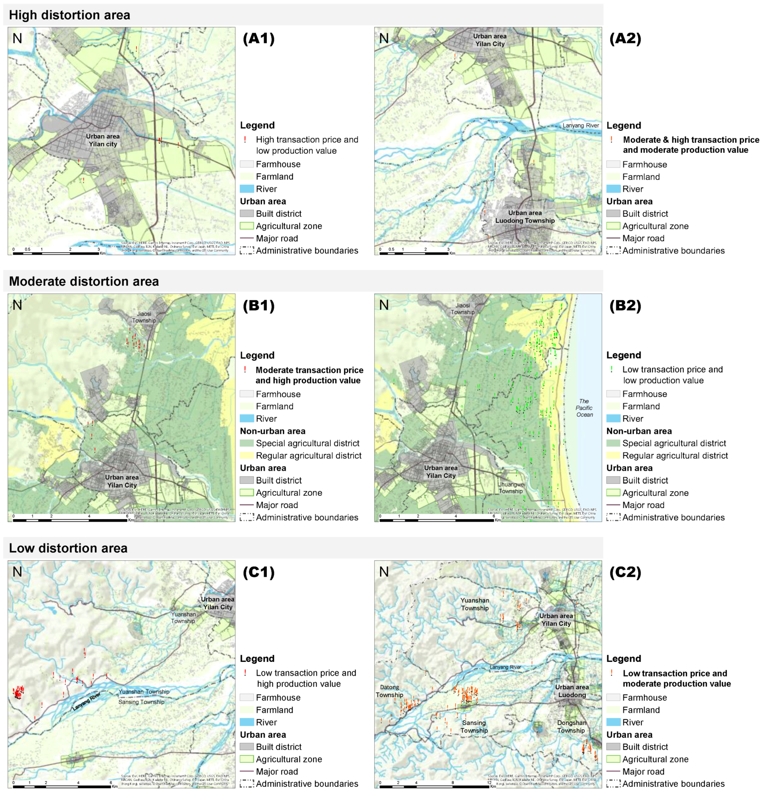
Cases of high distortion are shown in Figure 10 (A1,A2). Farmlands located in the agricultural zone of an urban area often have higher distortions due to their higher transaction prices and lower production values. This situation suggests a possibility of engendering an expectation for developing farmlands in urban areas. Development would destroy any opportunity of benefiting from the farmlands’ ecosystem services in urban areas because development is irreversible. Further, farmlands located in the special agricultural districts in the suburbs but in close proximity to urban areas often have higher transaction prices and production values; here, price-value distortions are moderate (Figure 10 (B1)) and there is serious conflict between farmland development and agricultural production.

Moderate distortions also occur when both the prices and production values of farmlands are low. This occurs in the regular agricultural district of suburbs (Figure 10 (B2)) and leads to a unique and widespread urban sprawl pattern in the rural areas of Yilan. Lower farmland price and higher production value generate low distortions, which occurs in the hilly area of Yilan County (Figure 10 (C1,C2)). Agricultural production in this area does not suffer from serious urbanization impacts. However, agricultural production itself has the potential to affect and pollute the environment through the use of fertilizers and pesticides. Clearly there are different cases of price-value distortion associated with the different farmland situations and characteristics, and these need to be taken into account by agricultural and urban planning departments of local and central governments. Therefore, a systematic approach of land administration is needed to consider the heterogeneity of these cases and inter-disciplinary cooperation from different departments in government is required [32].

5. Conclusions

Our findings indicate that policy reforms have significant impact on the farmland environment of Lanyang Plain and its surrounding regions. Investment in agricultural infrastructure was expected to improve production efficiency and increase production value. However, irrigation and road system improvements increased the price and thus the price-value distortion of farmland, which led to urbanization and impeded agricultural production in the region. The prices of farmland in agricultural zones within urban areas increased substantially due to speculation. This amplified the discrepancy between farmland price and its production value, which in turn increased the price-value ratio or distortion. Price-value distortion can be used as a proxy for the deviation between price and production value of farmlands, and can be mapped onto locations to explore reasons for the distortion and to understand its impact on agricultural development. Allowing non-farming use of farmlands can result in irreversible impacts on agriculture. Therefore, future urban planning has to consider the multi-functionality of farmland, and that the agricultural zone is not just for “reserving land for urban development.” Greater consideration of factors such as the multi-functionality of agriculture may provide a healthier balance between economic benefits and environment sustainability, as well as a finer balance between farmland price and value (Figure 11). Moreover, location assessment of farmland readjustment and agricultural investment policy should work with payment policy for the ecosystem services of farmland to decrease the distortion.

Land Administration Systems (LAS) can facilitate the sustainable development of farmland. LAS focuses land on systematic relations among various factors, ecosystem services and interaction between local and central governments [32]. The complex adaptive system can provide insights when deconstructing the complex agricultural landscape system in peri-urban area based on physical flaws and influence [33]. Additionally, Land Value Tax for non-agricultural use, real estate boom and recession may influence farmland price and distortion. It will be inspiring to employ these approaches to explore the spatial pattern of distortion ratio based on adequate and available transaction data in the future. Multifunctional use of farmland is absent from this study, but could be taken into account in future research.

References

- Gilg, A. Perceptions about land use. Land Use Policy 2009, 26, S76–S82. [Google Scholar] [CrossRef]
- Park, S.; Smardon, R.C. Worldview and social amplification of risk framework: Dioxin case in Korea. Int. J. Appl. Environ. Sci. 2011, 6, 173–191. [Google Scholar]
- Frumkin, H. Urban sprawl and public health. Public Health Rep. 2002, 117, 201–217. [Google Scholar] [CrossRef]
- Couch, C.; Petschel-Held, G. Urban Sprawl in Europe: Landscape Land Use Change and Policy; Wiley-Blackwell: London, UK, 2008. [Google Scholar]
- Chiang, Y.-C.; Tsai, F.-F.; Chang, H.-P.; Chen, C.-F.; Huang, Y.-C. Adaptive society in a changing environment: Insight into the social resilience of a rural region of Taiwan. Land Use Policy 2014, 36, 510–521. [Google Scholar] [CrossRef]
- Wang, C.-H. Analysis of Agricultural Land Change in Lanyang Plain Using a System Perspective; Chinese Cultural University: Taipei, Taiwan, 2014. (In Chinese) [Google Scholar]
- Wey, W.-M.; Hsu, J. New Urbanism and Smart Growth: Toward achieving a smart National Taipei University District. Habitat Int. 2014, 42, 164–174. [Google Scholar] [CrossRef]
- Plantinga, A.J.; Lubowski, R.N.; Stavins, R.N. The effects of potential land development on agricultural land prices. J. Urban Econ. 2002, 52, 561–581. [Google Scholar] [CrossRef] [Green Version]
- Hardie, I.W.; Narayan, T.A.; Gardner, B.L. The Joint Influence of Agricultural and Nonfarm Factors on Real Estate Values: An Application to the Mid-Atlantic Region. Am. J. Agric. Econ. 2001, 83, 120–132. [Google Scholar] [CrossRef]
- Kostov, P. A Spatial Quantile Regression Hedonic Model of Agricultural Land Prices. Spat. Econ. Anal. 2009, 4, 53–72. [Google Scholar] [CrossRef] [Green Version]
- McMillen, D. Conditionally parametric quantile regression for spatial data: An analysis of land values in early nineteenth century Chicago. Reg. Sci. Urban Econ. 2015, 55, 28–38. [Google Scholar] [CrossRef]
- Yoo, J.; Frederick, T. The varying impact of land subsidence and earth fissures on residential property values in Maricopa County—A quantile regression approach. Int. J. Urban Sci. 2017, 21, 204–216. [Google Scholar] [CrossRef]
- Chen, W.-B.; Lee, C.-L.; Chang, C.-R.; Wang, C.-H. An analysis of agricultural land change factors and spatial planning policies review for Lan-Yang Plain: The system approach. J. Taiwan Land Res. 2016, 19, 1–35. [Google Scholar]
- Huang, W.-S. The Farmland Price under Urbanization Pressure—A Case Study of I-Lan County; Department of Real Estate & Built Environment, College of Public Affairs, National Taipei University: Taipei, Taiwan, 2008. [Google Scholar]
- MA Synthesis. Ecosystems and Human Well-Being: Synthesis Report; Island Press: Washington, DC, USA, 2005. [Google Scholar]
- Stewart, P.A.; Libby, L.W. Determinants of Farmland Value: The Case of DeKalb County, Illinois. Rev. Agric. Econ. 1998, 20, 80–95. [Google Scholar] [CrossRef]
- Zhang, W.; Ricketts, T.H.; Kremen, C.; Carney, K.; Swinton, S.M. Ecosystem services and dis-services to agriculture. Ecol. Econ. 2007, 64, 253–260. [Google Scholar] [CrossRef] [Green Version]
- Bergstrom, J.C. Postproductivism and changing rural land use values and preferences. In Land Use Problems and Conflicts: Causes, Consequence and Solutions; Goetz, S.J., Shortle, J.S., Bergstrom, J.C., Eds.; Routledge: London, UK, 2005; pp. 64–76. [Google Scholar]
- De Groot, R.; Hein, L. Concept and valuation of landscape functions at diff erent scales. In Multifunctional Land Use: Meeting Future Demands for Landscape Goods and Services; Mander, Ü., Helming, K., Wiggering, H., Eds.; Springer: Berlin, Germany, 2007; pp. 15–36. [Google Scholar]
- Kong, F.; Yin, H.; Nakagoshi, N. Using GIS and landscape metrics in the hedonic price modeling of the amenity value of urban green space: A case study in Jinan City, China. Landsc. Urban Plann. 2007, 79, 240–252. [Google Scholar] [CrossRef]
- Lee, C.-L.; Lee, C.-H. Economic Assessments of Ecosystem Service Impacts of Agricultural Land-use Change (in chinese). Taiwa. Agric. Econ. Rev. 2012, 17, 111–144. [Google Scholar]
- Dehring, C.A.; Lind, M.S. Residential Land-Use Controls and Land Values: Zoning and Covenant Interactions. Land Econ. 2007, 83, 445–457. [Google Scholar] [CrossRef]
- Delbecq, B.A.; Kuethe, T.H.; Borchers, A.M. Identifying the Extent of the Urban Fringe and its Impact on Agricultural Land Values. Land Econ. 2014, 90, 587–600. [Google Scholar] [CrossRef]
- Faux, J.; Perry, G.M. Estimating Irrigation Water Value Using Hedonic Price Analysis: A Case Study in Malheur County, Oregon. Land Econ. 1999, 75, 440–452. [Google Scholar] [CrossRef]
- Beaton, W.P. The Impact of Regional Land-Use Controls on Property Values: The Case of the New Jersey Pinelands. Land Econ. 1991, 67, 172–194. [Google Scholar] [CrossRef]
- Wu, T.-C.; Lin, F.-T.; Lin, S.-T.; Hsu, Y.-L. Changes in Farmhouse Distribution Pattern and Factors Affecting Farmhouse Change in Yilan (in chinese). J. City Plan. 2013, 40, 31–57. [Google Scholar]
- Choumert, J.; Phélinas, P. Determinants of agricultural land values in Argentina. Ecol. Econ. 2015, 110, 134–140. [Google Scholar] [CrossRef] [Green Version]
- Henneberry, D.M.; Barrows, R.L. Capitalization of Exclusive Agricultural Zoning into Farmland Prices. Land Econ. 1990, 66, 249–258. [Google Scholar] [CrossRef]
- Papadimitriou, F. The Algorithmic Complexity of Landscapes. Landsc. Res. 2012, 37, 591–611. [Google Scholar] [CrossRef]
- Koenker, R.; Bassett, G. Regression Quantiles. Econometrica 1978, 46, 33–50. [Google Scholar] [CrossRef]
- Koenker, R.; Hallock, K.F. Quantile Regression. J. Econ. Perspect. 2001, 15, 143–156. [Google Scholar] [CrossRef]
- Williamson, I.; Enemark, S.; Wallace, J.; Rajabifard, A. Land Administration for Sustainable Development; Esri Press: California, CA, USA, 2010. [Google Scholar]
- Holland, J.H. Studying Complex Adaptive Systems. J. Syst. Sci. Complex. 2006, 19, 1–8. [Google Scholar] [CrossRef]
Figure 1.
Study area.
Figure 2.
Change in farmland price-value distortion.
Figure 3.
The farmland price-value distortion spectrum.