Climate Change, Agriculture, and Economic Development in Ethiopia


1
Potsdam Institute for Climate Impact Research (PIK), Member of the Leibniz Association, P.O. Box 601203, 14412 Potsdam, Germany
2
Institute of Transport and Economics, Technische Universität Dresden, 01062 Dresden, Germany
3
Humboldt-Universität zu Berlin, Department of Agricultural Economics, Unter den Linden 6, 10099 Berlin, Germany
*
Author to whom correspondence should be addressed.
Sustainability 2018, 10(10), 3464; https://doi.org/10.3390/su10103464
Submission received: 30 August 2018
/
Revised: 24 September 2018
/
Accepted: 26 September 2018
/
Published: 28 September 2018
(This article belongs to the Special Issue Climate Change and Sustainable Development Policy)
Abstract
:Quantifying the economic effects of climate change is a crucial step for planning adaptation in developing countries. This study assesses the economy-wide and regional effects of climate change-induced productivity and labor supply shocks in Ethiopian agriculture. We pursue a structural approach that blends biophysical and economic models. We consider different crop yield projections and add a regionalization to the country-wide CGE results. The study shows, in the worst case scenario, the effects on country-wide GDP may add up to −8%. The effects on regional value-added GDP are uneven and range from −10% to +2.5%. However, plausible cost-free exogenous structural change scenarios in labor skills and marketing margins may offset about 20–30% of these general equilibrium effects. As such, the ongoing structural transformation in the country may underpin the resilience of the economy to climate change. This can be regarded as a co-benefit of structural change in the country. Nevertheless, given the role of the sector in the current economic structure and the potency of the projected biophysical impacts, adaptation in agriculture is imperative. Otherwise, climate change may make rural livelihoods unpredictable and strain the country’s economic progress.
1. Introduction
Changes in the mean climatic conditions affect soil moisture, water availability, and the incidence and distribution of plant and animal pests and pathogens. These changes eventually lower agricultural productivity through their effects on crop growth [1,2,3,4,5,6], animal feed quality and quantity [6,7], and animals’ physiological performance [6,8,9]. Therefore, for a given set of inputs, climate change is analogous to technical change in agricultural production [6,10]. This will make rural livelihoods unpredictable in countries where agriculture is the main source of employment and income in rural areas. Consequently, climate change may trigger migration that involves changing residence locations (rural to urban) or changing economic sectors (agricultural to nonagricultural) or changing labor occupations (agricultural to nonagricultural) [11,12,13]. However, regardless of the form of migration, the end goal is to compensate the expected loss of income or to spread out risks [14,15]. Such productivity and migration effects in agriculture will propagate to the rest of the economy.
Sub-Sahara Africa is particularly susceptible to climate change due to the existing environmental conditions, least diversified and poor rural economies, and underdeveloped (but important in the macro-economy) agriculture [16,17,18]. Ethiopia is a typical case in this regard. Projections show that mean annual temperature and the number of hot days/nights will increase, and precipitation will be erratic but likely will decline in the country’s main crop growing season [19,20]. Such projections imply increasing evaporation and plant transpiration rates, decreasing soil moisture, and shorter crop/grass growing period [2] which all impose imminent risks to the country’s rain-fed and subsistence agriculture [20,21,22,23,24] and the macro-economy [25,26].
However, only a small share of previous studies on the economic impacts of climate change on least developed countries (LDCs) in general and on Ethiopia in particular apply general equilibrium models that are able to capture the induced and feedback effects of climate change on the whole economy. If available, most of the studies that apply general equilibrium models neglect migration, do not include regional effects (region defined as an administrative unit in a federal system), hardly deal with uncertainty of agricultural productivity changes and do not provide clear documentation on how they determine changes in agricultural productivity from crop models they employed e.g., [25,26].
We tackle some of these shortcomings in this paper. We examine the economy-wide and regional effects of shocks in agriculture due to future climate (2050s, average of 2035–2065) relative to the present climate (1990s, average of 1980–2010) in Ethiopia. First, we provide anticipated first-order effects of climate change on grain productivity, livestock productivity, and agricultural labor supply. Second, we modelled these first-order changes as changes in crop and livestock production efficiency and changes in labor supply in agricultural occupations in the computable general equilibrium (CGE) model. The results from the CGE model simulations are used to analyze the country-wide (economy-wide or general equilibrium) effects of climate change. Third, we project the sector-wise output effects simulated by the CGE model onto a regional module depicting the economic structure of different administrative regions of Ethiopia. This will help to glean information about the distribution of country-wide effects of climate change among different administrative units of the country. Fourth, we repeat the same CGE simulations of climate change impact scenarios while assuming some plausible cost-free exogenous structural change scenarios in the economy. In this regard, we specifically presume structural changes that improve labor skills (accruing to observed trends in education) and marketing margins (accruing to observed trends in transport and communication networks) in the economy. We do so to highlight the role of structural change to the resilience of the overall economy to the effects of climate change.
Our study makes several contributions to the literature. First, it links yield projections from crop models with an economic model for a developing country. Second, it incorporates climate change-induced yield changes in all grain commodities and apply an easy-to-use method to estimate climate change-induced productivity change in the livestock sector. Third, it adds migration on top agricultural productivity changes and complement the economy-wide analysis with regional analysis. Fourth, it contributes to the debate on development (structural change) as a generic climate change adaptation measure in LDCs. We believe the set of experiments in this paper gives a better picture of the economic effects of climate change in a low-income country. To the best of our knowledge, this is the first attempt to address this set of questions altogether in one paper for Ethiopia and other LDCs. Besides, our research design can easily be adapted to the case of other LDCs where a basic CGE model is already available.
2. Materials and Methods
2.1. Climate Change Impact Scenarios
We retrieved historical and future crop and grass yield projections from the Agricultural Model Intercomparison and Improvement Project (AgMIP) from [27]. Uncertainty is inherent in climate change impact projections. It accrues to one or more of the combinations of: the emission scenarios, climate models, and biophysical impact models used in the projections. Nevertheless, as shown by the Representative Concentration Pathways (RCPs), large differences are not expected among different emission scenarios until the 2050s [28]. Additionally, for a specific crop, crop models imply wider uncertainty than RCPs or Global Climate Models (GCMs) [29]. We checked and found both arguments to be tenable. Therefore, for this study, we found yield projections by different crop models are better to gauge the uncertainties in biophysical impacts.
This study is an economy-wide study. Therefore, we focus on the combinations of RCP, GCM, and global gridded crop models (GGCMs) that give us larger numbers of crop and grass yield projections. In light of this, we find the yield projections of the Lund-Potsdam-Jena managed Land (LPJmL) and the Environmental Policy Integrated Climate (EPIC) crop models under HadGEM2-ES climate model and RCP8.5 emission scenario to be better. The structural difference between the two crop models [29,30] was an additional advantage to account for uncertainties. The yields are projected with or without CO2 fertilization effects, and under no- or full-irrigation scenarios. We take the yield projections with no-CO2 fertilization effects since the actual benefits of CO2 fertilization effects are vexed [30]. We also take the yield projections with no-irrigation scenarios, partly because the current agricultural production system in Ethiopia is virtually rain-fed [31,32] while it is unlikely for the country to reach full-irrigation scenarios in the next two decades. Furthermore, we want to focus on the vulnerability of an economy where about 90% of the total agricultural production comes from rain-fed smallholder agriculture [33]. Irrigation, among others, would be a policy scenario to adapt to climate change which we leave to future research. Taken together, we consider two climate change impact scenarios. The differences between the scenarios are basically due to the crop models. Therefore, for simplicity, we hereafter refer to the climate change impact scenarios as LPJmL and EPIC scenarios. We acknowledge, due to our choice of the RCP, GCM, CO2 fertilization, and irrigation scenarios, the focus in this study is on high-end impacts as if the current agricultural system remains unchanged.
2.2. Climate Change and Crop Productivity
The AgMIP-GGCMs simulate yields for globally important crops at a spatial resolution of 0.5 × 0.5 degrees (approx. 50 × 50 km at the equator) [29,30]. Therefore, we took further steps to map the yield projections by AgMIP-GGCMs into our CGE model. First, we retrieved the mean annual yields projected using LPJmL and EPIC crop models under current (1990s: 1980–2010) and future (2050s: 2035–2065) climates from [27]. We chose 2050s as our future climate period to be consistent with the literature, e.g., [5,22,26]. The LPJmL model is applied to maize, millet, cassava, groundnut, peas, sunflower, rapeseed, rice, soybean, sugar beet, sugarcane, wheat, and managed grass. The EPIC model is applied to barley, maize, millet, dry bean, cassava, cotton, groundnut, sunflower, rapeseed, rice, sorghum, soybean, sugarcane, and wheat. Some of the AgMIP-GGCM crops however are economically less important in Ethiopia (e.g., rice and cassava) while some others are not directly represented in the country’s economic accounts (e.g., potatoes and sugarcane). On the other hand, many crops are cultivated in Ethiopia, some of which are local but economically important (e.g., teff and enset).
Second, therefore, we need to map the AgMIP-GGCM crops to the crops in the Ethiopian Social Accounting Matrix (SAM). We first established similarity between the crops on the basis of their photosynthetic pathway and the main climatic zone suitable for them [2,30]. Barley, teff, and wheat grow in areas with mild temperature and reliable rainfall [31,32]. The AgMIP-GGCM soybean and field peas are included in pulses of the Ethiopian SAM [31,32,34]. The AgMIP-GGCM groundnuts, rapeseed and sunflower are included in oilseeds of the Ethiopian SAM [31,32,34]. Based on 20 years of yield data from the Central Statistical Authority [35], we find the correlation coefficients between the yields of the aforementioned ‘similar’ crops to be high enough (r ≥ 0.85). Accordingly, for example, one can take barely or wheat yield change simulated by an AgMIP-GGCM as a proxy to teff crop yield change. However, the yield projections and changes may be sensitive to the crop model artifacts in case the crop model simulates with very low reference productivity [5,30]. Therefore, in order to control sensitivity to such variations, we imposed upper (+30%) and lower (−30%) caps to yield changes due to climate change (see also [5,30]). The mapping exercises help us to obtain climate change-induced yield changes for of all of the seven grain commodities in the original 2006 SAM of Ethiopia [34].
The procedures undertaken above give rounded up weighted average capped grain yield changes of −10% and −26% in LPJmL and EPIC scenarios, respectively. The weights are the share of each grain crop in the total grain cropland [31,32]. The average and single crop capped yield changes in this study are also in the range of yield changes reported in global [30] and regional [1,3,5] studies. Finally, in the calibrated CGE model, we modelled these grain yield changes as shocks to the total factor productivity (scale) parameter of the value-added component of the grain activity.
2.3. Climate Change and Livestock Productivity
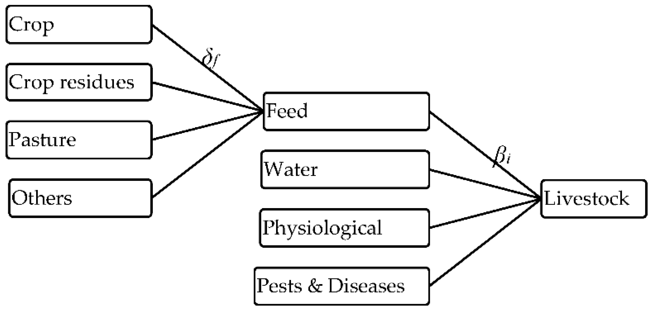
Climate change affects livestock productivity directly (e.g., through effects on growth, physiological performance, and immunity) and indirectly (e.g., through changes in the quality and quantity of forage, water availability, and pests and diseases) [6]. Unlike for the case of crops, however, there are no publicly available large-scale physiological models that directly link climate change and livestock productivity [36,37]. In spite of this, some, e.g., [8,9] argue that the indirect effects are the main channels through which climate change affects the smallholder livestock production sector in sub-Sahara Africa.
As such, we employ a simple approach that links climate change, animal feed quantity, and livestock productivity. The approach is important because about 87% of the total animal feed in Ethiopia, i.e., 59% green fodder (from grazing land) and 28% crop residue (from cropland) [31,32] is highly susceptible to climate change. The procedures presented in Section 2.2 give the effects of climate change on grain and grassland yields. We assume these yield changes, weighted by their respective shares in the total animal feed, can represent the effects of climate change on animal feed quantity. However, the changes in feed quality and quantity represent only a portion of the total effects of climate change on livestock productivity. We merely assume this channel accounts for about 30% of the total effects of climate change on livestock productivity. Accordingly, we multiplied the total feed quantity change due to climate change (which we assume is directly proportional to weighted yield changes) by 0.3 to obtain climate change-induced livestock productivity changes. We have provided further notes in Appendix A.
The procedures result in livestock productivity changes of −2% and −5% in LPJmL and EPIC scenarios, respectively. In the calibrated CGE model, we introduced these changes as shocks to the total factor productivity (scale) parameter of the value-added component of the livestock activity.
2.4. Climate Change and Agricultural Labor Migration
Climate change may trigger rural-urban migration or movement of labor from agricultural to the non-agricultural sectors/occupations [11,12,13]. However, it still remains hard to explicitly untangle the exact numbers of climate change-induced migrants between locations, sectors, or occupations [14,15]. The other constraint in modelling climate change-induced migration stems from the structure of the model at hand and its benchmark data. In light of this, just to be consistent with the labor factor accounts in the SAM, in this study we consider and model migration as the movement of labor between occupations (or labor segments). However, data on migration between economic sectors or labor segments is still hardly available. Therefore, we extrapolate such migration between occupations based on the macro- and micro-evidence of rural-urban migration in Ethiopia.
In general, previous country level reports, e.g., [38,39,40,41] and micro-level studies, e.g., [42,43,44,45,46,47] attribute rural-urban migration to the fast growing population, environmental degradation, low agricultural productivity, and recurrent droughts and famines in rural areas. For instance, between 1999 and 2013, recent migrants that attribute their main reason of migration to the shortage of agricultural land rose by 240% in urban areas and by 50% in rural areas [38,40]. Likewise, migration rates of males are found to be 1.4% and 2.6% during periods with no droughts and with severe droughts, respectively [43]. Land shortages and crop failure and related economic problems are the main drivers of rural-urban migration in Woldyia town [44] and Damot Galie district [42]. At country level, droughts and agricultural land shortages are reasons for about 0.15 million of the total 3.8 million recent migrants [38]. Many such migrants are bound for urban areas contributing to the increasing rural-urban migration trend in Ethiopia. For example, between 1999 and 2013, while the total recent migrants increased by 67%, the number of rural-urban recent migrants rose by 130% [38,40]. As a result, the rural-urban migration is catching up the rural-rural migration which has been the dominant form of migration for decades. In 2013, the rural-urban migrants accounted for 33% (up from 24% in 2005) of the total recent migrants whereas rural-rural migrants accounted for 35% (down from 46% in 2005) [38]. Similarly, the Ethiopian government resettled more than 0.5 million households in response to the infamous 1984/85 drought that affected mainly northern Ethiopia [47].
On the basis of the aforementioned micro-level case studies, national labor surveys, and population censuses, we assume that the crop and livestock productivity shocks due to LPJmL and EPIC climate change impact scenarios may, respectively, cause a migration of 0.5 and 1 million workers from agriculture. In the CGE model, we modelled this climate change-induced migration as an exogenous phenomenon that reduces labor in agricultural occupations (or agricultural labor segment) but increases labor in elementary occupations (or unskilled labor segment) by the same amount of labor. The elementary occupations include occupations that require no specific skills [34]. The aforementioned migration numbers correspond to shocks to agricultural labor supply (LPJmL = −2% and EPIC = −4%) and to unskilled labor supply (LPJmL = +36% and EPIC = +73%) compared with the corresponding observed labor supplies in the calibrated CGE model [39]. Our main focus here is on the general equilibrium effects of migration that accrue to factor substitution effects and relative wage changes in the CGE model. It requires no further information about the specific activities and regions of origin and destination of the migrants. The migrants from agriculture can still stay in rural areas and work in cottage manufacturing industries (such as weaving, tanning, grain milling, and the like).
2.5. Structural Change Scenarios
Ethiopia has experienced rapid economic growth and urbanization rates in the past decade [41,48]. In particular, the county has made promising progress in education, transport, and communications sectors where also the government plans to continue its substantial investments [48,49,50]. The past and planned trajectories in these sectors will foster structural transformation in the economy [49,51]. Development in these sectors will, among others, ease the rigidities in the labor market and reduce the trade and transport margins on market commodities. Accordingly, we construct some plausible structural change scenarios to highlight the role of such anticipated changes in the economy to dampen the adverse consequences of climate change. We treat these structural change scenarios as cost-free exogenous changes that simultaneously occur with climate change in the calibrated CGE.
2.5.1. Improving Labor Skills
We assume that the observed trends in the education sector, among others, may reduce the skill differences among different labor segments/occupations. The labor occupations in the SAM (and, hence, in the calibrated CGE model) are constructed on the basis of labor skills [34]. The occupations can broadly be categorized as agricultural and non-agricultural occupations. The latter group of occupations include unskilled workers (FLAB3 hereafter), skilled workers (FLAB4 hereafter), professional and technical workers (FLAB2 hereafter), and administrative workers (FLAB1 hereafter). The classification and notation of the labor segments/occupations here are the same as in [34] just for the sake of easy correspondence. Accordingly, the FLAB4 workers possess some skills obtained through formal and informal education, training, and experience but apparently lower (or other) than skills required for FLAB2 and FLAB1 occupations [34]. Note that in this paper we are using labor segments and occupations interchangeably.
Our argument here is that structural change will ease labor mobility among different occupations, for instance, from agricultural occupations to non-agricultural occupations. Accordingly, we construct a set of four structural change scenarios that represent different levels of changes in the skills of the present agricultural workers. Under this set of experiments, for a portion of agricultural workers (FLAB0 hereafter), skill is no more a constraining factor to transfer to other labor segments. When the agriculture sector is affected by exogenous factors (e.g., by climate change), that same portion of agricultural labor can easily move to either of the non-agricultural labor segments.
We can model these phenomena as decreasing agricultural labor supply but, increasing, the labor supply in other labor segments by the same numbers of workers. The strength of the presumed trajectories in education and training would determine the destination occupation. With no structural change assumed, the movement would be from farming (FLAB0) to elementary (i.e., FLAB3) occupations as farmers usually do not possess skills other than farming. This is what we do in Section 2.4. It will be our benchmark scenario to see the dampening effects of other labor movement scenarios corresponding to structural change scenarios (i.e., from FLAB0 to FLAB4, FLAB2, and FLAB1). The total labor supply in the economy remains fixed at the observed level in all scenarios of migration between occupations. Absence from the labor market at the time of education and training, the period of time required to finish and attain the set of skills to fit to a specific labor segment, and similar issues are beyond the scope and objectives of this study. However, structural change may also help to harness opportunities that may arise from the demographic structure of the country. The net labor supply in Ethiopia has been positive every year as about 45% and 3.5% of the total population in Ethiopia are aged below 15 and above 65 years, respectively [38]. Therefore, we construct another set of five experiments to represent the case with education and training that exclusively focuses on about 0.5 million currently economically inactive peoples. Each experiment represents the occupational group where the extra labor force will be allocated to. The benchmark among this set of experiments would be allocating the extra labor force to agricultural occupations so that the benefits due to structural change can be distinguished from the benefits due to increase in the total labor endowment of the country.
2.5.2. Declining Marketing Margins
Ethiopia has remarkably invested in transport and communication infrastructures in the past two decades [51] as a result of which domestic market integration is increasing, marketing margins are declining, and regional price disparities are narrowing [48,49]. In line with this, we consider a structural change scenario in which the marketing margins (i.e., transport and trade margins) in all marketed commodities decline by ten percent. This is particularly relevant for agricultural markets where inadequate transport and communication networks are the major setbacks. For example, about 83% of the gross grain marketing margins accrue to physical marketing costs related to transport, handling, and other marketing activities [52]. Likewise, [53] finds that transport costs account for 6–21% of market prices per quintal of maize, sorghum, and millet in rural villages surrounding Atsdemariam town in north west Ethiopia.
The summary of different climate change impact scenarios discussed so far are given below in Table 1. Each scenario correspond to a CGE simulation.
2.6. The CGE Model Calibration and Regional Projections
We apply the static IFPRI-CGE model [54]. While a dynamic version of the IFPRI-CGE model is applied in [55], we prefer the static version of the model since the projected biophysical effects in specific time are relatively uncertain compared with the average effects over a period of time. Consequently, the economic effects of climate change using dynamic models are much more prone to uncertainties compared with those effects using static models. Additionally, in general, dynamic models make it hard to distinguish the economic effects of climate change that attribute to the projected climate change (and the related uncertainties) from those effects due to the projected socio-economic changes (and the related uncertainties) [56] which may have implications for the timing, the scale, and the types of adaptation measures.
The CGE model database is the 2005/06 SAM of Ethiopia [34]. However, we modified the original SAM into 54 total accounts that consist of 17 activity, 18 commodity, eight factor, two household, three tax, and six other accounts (enterprise, government, ROW, savings-investment, changes in stock inventory, and transport and trade margin). Our calibration of the model involves of a nested production technology, a range of elasticities, a factor market closure, and a combination of macro-closures that are common in the empirical CGE modelling for developing countries. The trade, income, and factor substitution elasticities are collected from the related literature. We construct a satellite account for the physical units of each labor type, cropland, and tropical livestock units (TLU) employed in each SAM activity based on data from the 2005 National Labor Force Survey [39] and Annual Agricultural Sample Survey [32].
The CGE model is used to simulate the economy-wide effects of different climate change impact scenarios presented in Table 1 above. We present and analyze the economy-wide effects, especially on the macro-economy, sector-wise output, and households’ welfare. We further project the sector-wise results onto a regional module. These kind of regional projections help us to glean information on the regional distribution of the effects of the climate change modelled at country-wide level. In general, in the Ethiopian context, it can be argued that the economy-wide representative agents (and markets) fairly represent the regional representative agents (and markets) [51,57]. Nevertheless, the administrative regions—nine regional states and two city administrations—vary in terms of their economic structure and share in different country-wide socio-economic indicators. Under such conditions, regional disaggregation and analysis based on CGE results have enormous policy relevance [58].
The regional analysis approach that we pursued here is a top-down approach comparable with the ORANI Regional Equations System (ORES) for Australia [59]. However, unlike the ORES-Australia which explicitly classifies regional industries (activities) as ‘national’ or ‘local’, we consider all regional activities in all regions to be ‘national’ activities [58,59]. The ‘national’ activities produce commodities tradable among regions of the country, thus, the demand for commodities of ‘national’ activities comes from the whole country regardless of the regional location of the activities: Whereas the ‘local’ activities produce commodities which are non-tradable across regions, thus, the demand for local commodities comes only from the region where they are produced [58,59,60]. To overcome the data availability problems, we assume that regional shares of all sectors in country-wide sectoral outputs remain constant. By implications, output of a sector in all regions changes proportionally to the changes in the country-wide output of the same sector. However, since the contribution of each sector to the total regional output varies across regions, the overall effect of an exogenous change will be different across regions.
Unfortunately, there are no data for regional sector-wise and region-wide GDP in Ethiopia. We took a remedial measure here. We compute sector-wise and region-wide value-added GDP directly from the SAM [34] complemented with employment data from different sources [32,39,61,62]. Our approach resolves both data availability and consistency problems. It is not necessary to modify the CGE model as long as the activities of the SAM are made consistent with the activities of the micro-surveys used to construct the regional shares. Nonetheless, our approach requires a strong assumption of labor intensity (and production technology in general) of an industry is the same regardless of the administrative region in which it is located.
Taken together, other things remaining constant, the regional effects are determined by the nature of the CGE experiments (that reflect the sign and strength of sector-wise effects at country level) and the economic structure of the regions (that show the importance of each sector in different regions).
The details of the CGE model, the calibration procedure, and the regional module are presented in Appendix A.
3. Results and Discussion
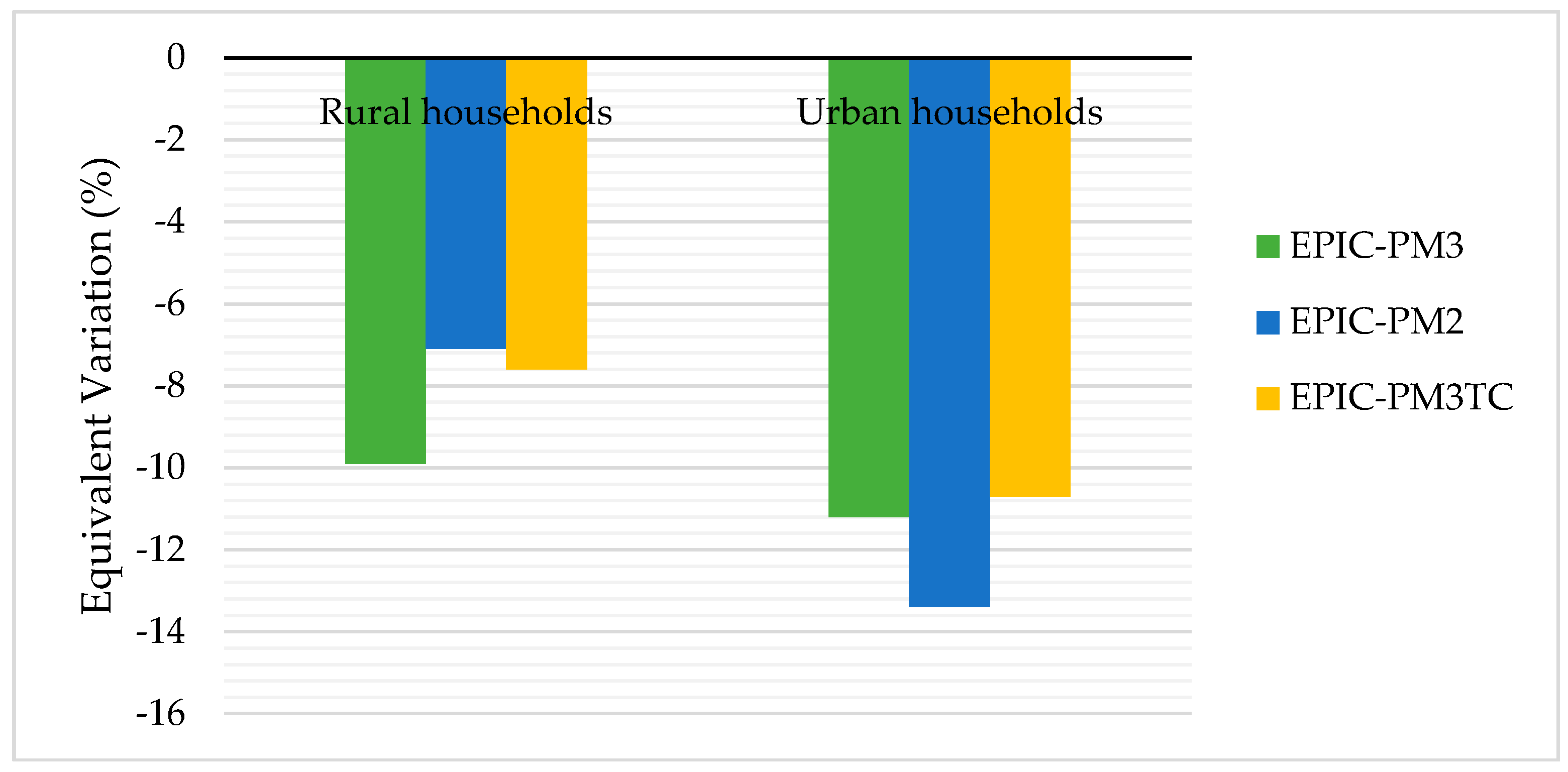
In this section, we present and discuss the effects of climate change on the macro-economy (e.g., on GDP, total private consumption, exports, and imports), sector-wise outputs, households’ welfare, and the value-added GDP of different regions. The change in household welfare is represented by the equivalent variation (EV) which measures the difference between the utility of a household before and after an exogenous change occurred.
3.1. Economic Effects of Climate Change without Structural Change
3.1.1. Country-Wide Effects
The CGE results show that total private consumption and exports decline in a range of 0.3% to 9% and 2.8% to 7.8%, respectively. The country-wide GDP declines by 2.6% to 8% which is larger than the decline in total absorption (2% to 6.5%) indicating that imports may help to dampen the macroeconomic effects of climate change [26,55]. The macroeconomic effects of the migration scenarios are negligible.
As one would expect, climate change hits agricultural activities hard (see Table 2). The effects on grain output could reach −26% under EPIC-PM3 scenario. Table 2 also shows that the climate change-induced shocks to grain and livestock activities ripple through the rest of the agricultural activities (e.g., enset crop, cash crops, and fishing and forestry). This may be explained by the increasing competition for cropland and agricultural labor. The shocks to the agricultural labor supply (i.e., migration only) cause proportional decline of agricultural output contrasting the micro-level studies which find no or little effects of migration on agricultural output [63,64]. The contrasts may be because the aforementioned studies did not consider general equilibrium effects. With increasing shocks to agricultural productivities, the repercussions spread further to non-agricultural activities that use agricultural commodities as intermediate inputs (e.g., hotels and restaurants, and construction) and to the wholesale and retail trade as agricultural commodities contribute to the total traded output in the economy.
Domestic agricultural prices will increase as a result of declining agricultural output. Consequently, the ratios of domestic prices to international (export and import) prices of agricultural commodities increase. As a result, agricultural exports decrease whereas agricultural imports increase. Since the macroeconomic trade balance is fixed, by the virtue of the macro closure rules used in calibrating the model, the decrease/increase in exports/imports of agricultural commodities shall be balanced by the increase/decrease in exports/imports of non-agricultural commodities. Accordingly, output from non-agricultural activities shall increase to fill the export gap due to decline in agricultural exports (e.g., from manufacturing, transport and communications, and ‘other’ services) and to meet the domestic demand gap due to decline in imported varieties of non-agricultural commodities (e.g., from manufacturing and mining). Therefore, in Table 2, we see increasing output in some non-agricultural activities such as manufacturing (2.5% to 13%), transport and communications (1% to 6%), ‘other’ services (1% to 13%), and minerals and quarrying (1% to 5%). Table 2 also shows that activities which employ the bulk of unskilled labor (e.g., manufacturing and ‘other’ services) will expand further under migration scenarios. Migration could also offset some of the ripple effects due to productivity shocks in agriculture in mining, trade, and hotels and restaurants in which non-negligible share of unskilled labor type is employed. One would argue that the repercussions on the rest of the sectors are weak in general. Three main features of the economy explain it. First, the factor reallocation effects between agriculture and non-agriculture sectors are rather negligible. The majority of factors of production in agriculture (cropland, livestock, and agricultural labor) are used only in the agricultural sector. Second, the interlinkage between agricultural and nonagricultural activities is rather weak. On the one hand, only a fraction of agricultural output is available to be used as intermediate input in other sectors as the majority of agricultural output is used by rural households (as home commodities) and by the sector itself (as seeds). On the other hand, the main industrial input to agriculture (i.e., fertilizer) is entirely imported. Third, the ripple effects through changes in relative commodity prices—changes in agricultural prices relative to non-agricultural prices—are also disposed to be low. On the one hand, as a low-income country, the income elasticities are low. On the other hand, the model assumes that the objective of each household group is to maximize its utility specified by a Stone-Geary function which results in a linear expenditure system (LES) of consumption demand. The LES implies low own- and cross-price elasticities as well as gross complementarity among commodities [65].
The effects of climate change on commodities (supply and price) and factors (demand and wages) eventually influence households’ welfare. Figure 1 shows welfare effects to urban households (−0.3% to −11%) and to rural households (−0.3% to −10%). The urban households are relatively worse off because they are subject to changes in output as well as changes in consumer prices of agricultural commodities compared with rural households who produce and consume the vast majority of agricultural commodities [31,32,34]. Recall that we modelled migration as movement of labor from agricultural to elementary occupations. As per the SAM [34] and the calibrated CGE model, the vast majority of unskilled labor is employed in manufacturing and services which are commonly located in urban areas. Therefore, as shown in Figure 1, the welfare loss of both household groups get worse when migration is added on top of productivity changes. The marginal welfare loss due to migration to rural households and to urban households is, respectively, explained by the decline in total agricultural output (and hence decline in total agricultural income) and by the decline in urban wage rates due to increase in labor supply, and the marginal increase in agricultural prices.
The effects on households’ welfare discussed here, as in any CGE model applications, are also influenced by the values of the parameters and the macroeconomic and factor market closures used to calibrate the model. First, the income, own- and cross-price elasticities of demand are rather low. Second, the calibrated model distinguishes between home commodities (valued at producer prices) and market commodities (valued at sales prices). Accordingly, the vast majority of agricultural commodities are home commodities for rural households. Third, we impose a minimum (mandatory) consumption requirement for both of the household groups. These are common practices in CGE modelling for LDCs. The forgoing aspects of the calibrated model control the responsiveness of the households’ consumption spending to the changes in incomes of households and prices of commodities. In effect, households’ welfare changes are smaller than changes in agricultural outputs and prices. The implication is that Ethiopian households would rather use their savings to smoothen their consumption during the times of exogenous shocks. In this regard, the CGE results corroborate the findings of [45,66] according to which Ethiopian households usually sell their assets during the periods of droughts.
Altogether, the economy-wide results show that the primary effects of climate change on agriculture have profound effects on the macro-economy (e.g., GDP, private consumption, and exports) and households’ welfare. This reflects the macroeconomic importance of agriculture in Ethiopia. The repercussions on other sectors, however, are not as strong as one would have expected because of the structural features of the economy.
3.1.2. Regional Effects
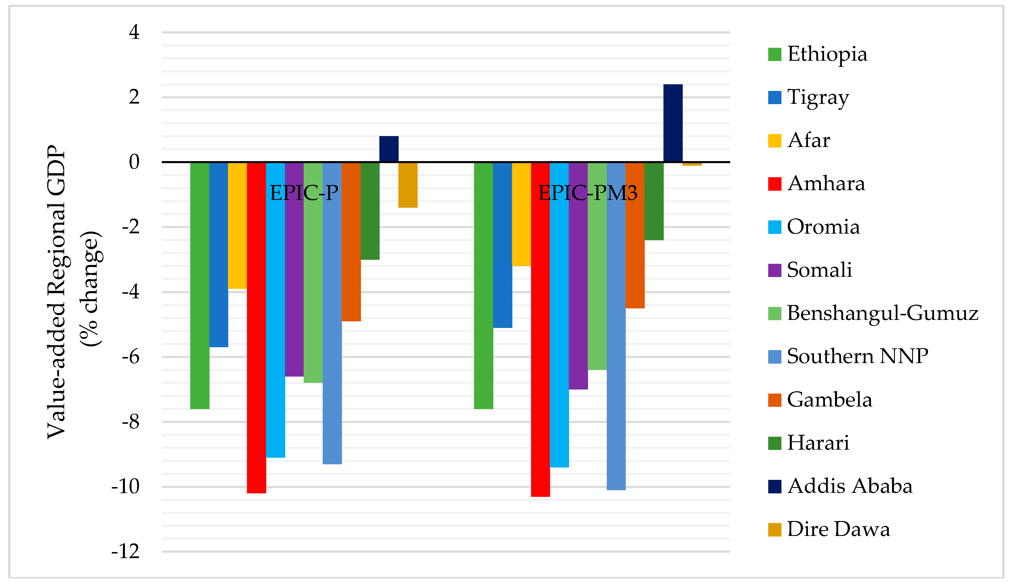
The regional effects of climate change-induced shocks to agricultural productivity range from −4.1% to +1.1% in the LPJmL scenario, and from −10.3% to +2.4% in the EPIC scenario. The effects are adverse and strong in the three largest agrarian regions of the country which include Oromia, Amhara, and Southern Nations, Nationalities, and Peoples (Southern NNP) states. In contrast, the effects are relatively low in urbanized regions, i.e., in regions where more than 50% of the total population lives in urban areas. According to [61] Addis Ababa (100%), Dire Dawa (68%), and Harari (55%) are the three most urbanized regions of Ethiopia. The share of urban population in Ethiopia in the same year was barely 16% [61]. The changes in Addis Ababa city are favorable under all impact scenarios. This is explained by the negligible share of agriculture and high share of manufacturing and services in the city’s value-added GDP (see Table 2 above and Table A2 in the Appendix). In regions where non-agricultural industries make significant contribution, climate change-induced migration between occupations may dampen the effects due to productivity shocks. This is reflected mainly in Addis Ababa, Dire Dawa, and Harari, and to some extent in Tigray and Afar regions. The effects of occupation migration are the other way around in Southern NNP, Amhara, Oromia, and Somali regions. This implies that agricultural labor migrants from agrarian regions may end in the manufacturing and services sectors of the urbanized regions. The results somehow go with the observed evidence. For example, the net migration rate per 1000 people is positive in Addis Ababa (430) and in Dire Dawa (289) but negative in Amhara (−64) and in Southern NNP (−27) [39]. Nevertheless, the CGE results shall be interpreted with caution as we do not consider the direct and indirect costs of migration to the receiving regions. If such costs are high, they probably are, climate change-induced migration will have negative consequences for the regions of origin (i.e., agrarian regions) and of destination (i.e., urbanized regions). This may be a subject of future research.
Figure 2 depicts that the regional effects of climate change depend on the region’s own economic structure as well as its structure relative to the national economic structure. For instance, Tigray is an agrarian region. However, according to our regional module, the share of grain activity in Tigray is relatively smaller than the share of grain activity in Ethiopia. It follows from this that the effects of climate change on Tigray-wide GDP are smaller than those effects on Ethiopia-wide GDP. In addition, the regional effects with occupational migration (EPIC-PM3) tend to be lower than the regional effects of productivity shocks (EPIC-P) in Tigray, Afar, and Harari regions. This is explained by the existence of other sectors (in addition to grain and livestock) which make important contributions to their regional GDP (see Table A2 in the Appendix). This highlights the role of diversification to dampen regional effects of climate change, for example, through employing migrants from agriculture in manufacturing and service sectors within the same region.
3.2. Economic Effects of Climate Change with Structural Change
We go further to investigate the role of cost-free exogenous structural change scenarios (discussed in Section 2.5) to offset the adverse effects of climate change (discussed in Section 3.1). We particularly present the case of EPIC impact scenario.
3.2.1. Country-Wide Effects
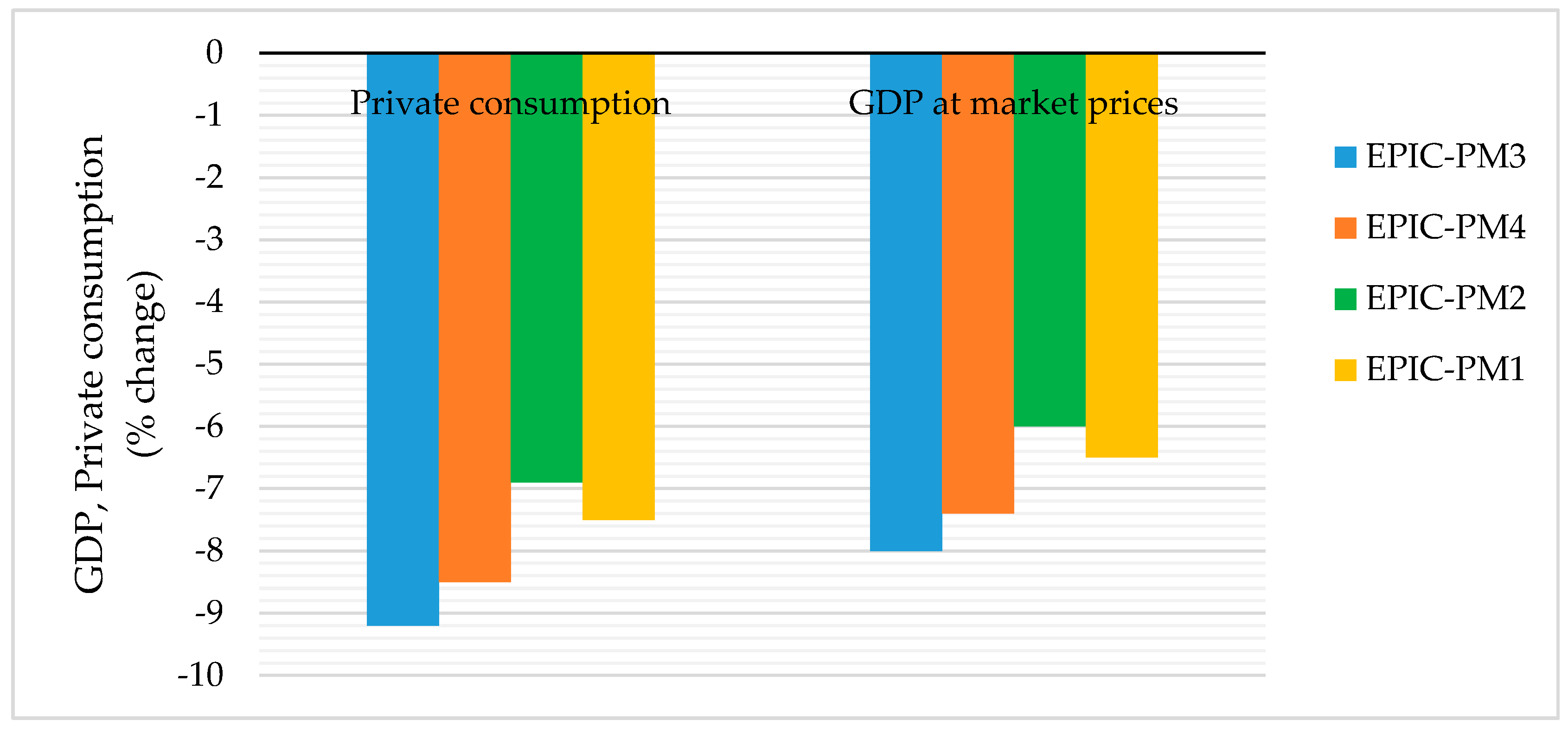
The effects of climate change get relatively smaller if the skills of the present labor force would improve. Compared with the benchmark migration scenario (EPIC-PM3), migration of agricultural labor to the skilled (EPIC-PM4), to the professional and technical (EPIC-PM2), or to the administrative (EPIC-PM1) labor segments would dampen the adverse effects on the Ethiopia-wide GDP by about 20–30%. Migration to occupations other than elementary occupations could also offset part of the aggregate private consumption loss caused by climate change. The offsets are vivid when agricultural labor moves to professional and technical occupations (see Figure 3). However, any form of occupational migration relatively increases/decreases the real wage rate of agricultural/non-agricultural labor following which the rural households/urban households are slightly better off/worse off compared with welfare effects discussed in the previous section (see Figure 1).
The results also suggest that the economy would be more climate-resilient, especially, if the future generation of labor force is directed towards professional and technical occupations. For instance, the effects of climate change on GDP under the scenario that one half million extra labor force are added to professional and technical occupations (−5.7%) is lower than the case of adding the same numbers of labor to agricultural occupations (−6.7%) or elementary occupations (−7%). The effects on total households’ welfare exhibit a similar pattern. It should, however, be noted that allocating the extra labor force to occupations other than agriculture may worsen urban households’ welfare.
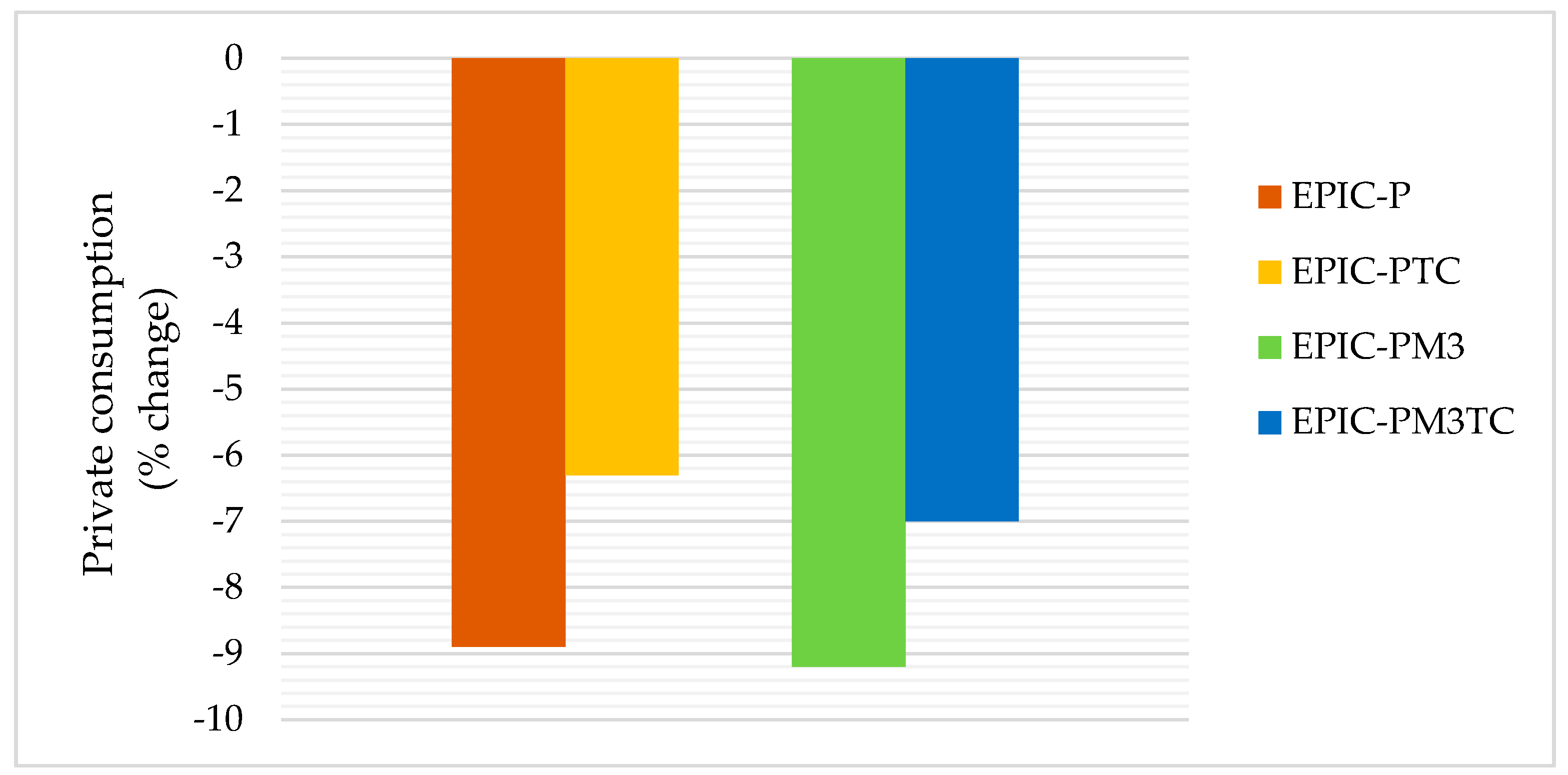
About 10% decline in marketing margins (or transaction costs) in all marketed commodities would offset the effects on total private (households) consumption by around two percentage points (see Figure 4). The offsets to the rural households are unambiguous (see Figure 1). This may accrue to the marginal increase in net agricultural revenue since, for instance, a decrease in marketing margins would increase domestic receipts from exports for a given set of international prices and volume of exports.
3.2.2. Regional Effects
The regional projections resemble the country-wide effects in many of the cases. Migration and allocation to professional and technical occupations imply better outcomes. The GDP of urbanized regions expand, particularly, under labor-oriented structural change scenarios. For instance, the effects on Addis Ababa’s GDP increase by one to five percentage points compared with the effects of climate change without assuming these structural change scenarios. This is expected with manufacturing and services which benefit from increased numbers of skilled labor types (i.e., FLAB4, FLAB2, and FLAB1) are the dominant economic sectors in Addis Ababa and other urbanized regions. Likewise, the allocation of the incoming labor force to non-agricultural occupations increases further the GDP of urbanized regions. For the agrarian regions (e.g., Southern NNP, Amhara, and Oromia), migration to other labor segments will slightly dampen (or leave unchanged) the effects due to climate change-induced productivity shocks. On the other hand, declining marketing margins affect the wholesale and retail trade output as it depends on the trade margins realized on all market-commodities. This is reflected in the regions of Harari and Dire Dawa. Despite this, declining marketing margins are still important to dampen the macroeconomic effects of climate change.
It is worth mentioning here that the structural change scenarios we assumed are not supposed to prevent (or even modify) the first-order effects of climate change in agriculture, and to change the macroeconomic relevance of the agricultural sector. What we aim to establish here is that climate change would continue to induce the primary effects in agriculture whereas the structural change scenarios would offset the ripple effects to the rest of the economy. The setup has two consequences. First, the effects of climate change in grain, livestock, and other agricultural activities are hardly dampened by the structural change scenarios. Second, the magnitude of the offsets are not so strong (only 20–30% in aggregate variables) compared with the fact that we did not account for the costs leading to such structural change scenarios. This is because we considered the role of structural change scenarios only in labor and commodity markets. The rest of the structural features of the economy including the macroeconomic relevance of the agricultural sector remains the same. By implication, structural change that simultaneously reduces structural rigidities in labor and commodity markets, and expands non-agricultural sectors would imply better resilience to climate change.
Taken altogether, the study results indicate that investments in education and training (to improve labor skills) and in market connectivity and efficiency (to reduce marketing margins) would contribute to climate-resilient economic development in Ethiopia. This can be regarded as a co-benefit of the current and future growth and structural transformation plans of the country [49,67].
4. Conclusions
We assess the economic consequences of the impacts of climate change on agricultural productivity and labor supply. The economy-wide (or CGE) analysis shows that climate change reduces agricultural output, increases agricultural price, alters the international trade mix, and profoundly affects households’ welfare. In many cases, the effects on total GDP and households’ welfare resemble those effects on agricultural GDP and rural households’ welfare. This reflects the macroeconomic importance of agriculture in Ethiopia. We find migration between occupations to cause negligible macroeconomic effects but important effects on agricultural output. We also find negligible indirect effects of climate change on non-agricultural sectors which can be attributed to the structural features of the economy which include: (1) weak inter-industry linkages, (2) using the bulk of agricultural output for rural household consumption, (3) low income and price elasticities, and (4) almost no competition between the agricultural and the non-agricultural sectors for the factors of production. We also find that the effects of climate change are uneven among administrative regions of the country. The effects are negative and strong in some agrarian regions (e.g., Amhara, Oromia, and Southern NNP) but positive in Addis Ababa and less adverse in other urbanized regions (e.g., Dire Dawa and Harari). Our regional analysis highlights that diversifying regional economies may help to harness opportunities that may come along with migration from agricultural occupations in the same region. Otherwise, migration from agriculture may widen regional disparities and impair the economic prospects of both sending agrarian regions (due to loss in productive labor) and receiving urban regions (due to pressure on real wage rates and urban infrastructure).
We find that our results with improving labor skill and declining marketing margin scenarios in general show that structural change may underpin the resilience of the Ethiopian economy to climate change. Nonetheless, the types of structural changes may matter for the regions. The offsetting effects of labor-related structural change scenarios lean towards urban regions while those of marketing margins lean towards agrarian regions.
We use different materials and methods compared with previous studies on the general equilibrium effects of climate change-induced agricultural productivity changes, e.g., [25,26,55]. Nonetheless, whenever the research questions are the same, our general results and conclusions corroborate the findings of the aforementioned studies and other studies on related topics, e.g., [45,66,68]. This leads us to conclude that the climate change risks to the Ethiopian economy are imminent irrespective of the materials and methods used. Our findings also show that structural change may contribute to climate-resilient development in the country corroborating the arguments raised elsewhere, e.g., [69,70,71,72]. As such, one would expect that the current economic growth and transformation plans of Ethiopia, e.g., [49,67] would contribute to the resilience of the economy to climate change. In balance, given the importance of the sector in the present economic structure, and the potency and the likelihood of the biophysical impacts, proactive adaptation in the Ethiopian agriculture is necessary. Otherwise, climate change may strain economic progress of the country [71] as the spectrum of adaptation in later periods may get narrower [1]. Therefore, policy makers should carefully design policy instruments that fairly allocate the country’s scarce public resources between public adaptation in agriculture and structural transformation measures. Promoting climate-resilient urban agriculture and large-scale commercial agriculture may have double-dividend in this regard. Future research in this line is needed.
Before closing, however, we want to point that the study is not without limitations. We considered only two impact scenarios which are definitely not enough to capture the range uncertainties in climate change projections and impacts. We were also compelled to focus only on grain crops as the application of crop models to simulate impacts on perennial crops is very limited to date. Due to this we are unable to include the likely effects of climate change in, for example, coffee, which is the single most important export item of the country. We also did not include effects that may arise from changes in international prices (e.g., of food imports) due to climate change impacts elsewhere in the world. Such effects can be included either by using global CGE models or integrating global partial equilibrium models of agriculture which have trade components with single-country CGE models. Most importantly, we employed rather simplistic approaches in some aspects, especially in livestock productivity, migration, and structural change. Future research to refine these approaches, particularly using empirical evidence and data, is badly needed.
Author Contributions
A.W.Y. conceived the paper, curated the data, designed the methodology, run the simulations, analyzed the results, wrote the first draft of the paper, and revised the paper. G.H. provided crucial inputs to the design of the methodology and simulations, to the analysis of the results, and revised the first draft of the paper. H.L.C. provided crucial inputs to the design of the methodology and simulations, to the analysis of the results, and reviews to revise the paper. S.T. provided reviews in each stage of the paper. All authors read and approved the final manuscript.
Funding
A.W.Y. is grateful to the financial and research support from Dresden Leibniz Graduate School (DLGS) and Leibniz Institute of Ecological Urban and Regional Development (IÖR). The publication of this article was partially funded by the Open Access Fund of the Leibniz Association.
Acknowledgments
We would like thank Christoph Müller at Potsdam Institute for Climate Impact Research (PIK) for clarifying our questions with regard to the biopsychical models and impacts.
Conflicts of Interest
The authors declare no conflict of interest.
Appendix A.
Appendix A.1. Livestock Productivity Changes
Livestock productivity changes due to climate change are linked to climate change-induced grain and grass yield changes.
Figure A1.
Conceptual framework of climate change impacts in the livestock sector. δf and βi stand for the share of a specific feed type in total animal feed and for the share of a specific impact channel through which climate change affects livestock production. Source: Authors’ illustration.
Figure A1.
Conceptual framework of climate change impacts in the livestock sector. δf and βi stand for the share of a specific feed type in total animal feed and for the share of a specific impact channel through which climate change affects livestock production. Source: Authors’ illustration.

The specification we apply is as follows.
Appendix A.2. Brief Description of the CGE Model Structure and Calibration
We apply the static IFPRI-CGE model [54]. The main features of the model are the followings:
- Perfect competition in commodity and factor markets.
- A small-open economy with respect to international trade.
- Imperfect transformation between domestic sales and exports, and imperfect substitution between domestic output and imports.
- Producers, households, enterprises, government, and rest of the world represent decision-making nodes in the CGE model.
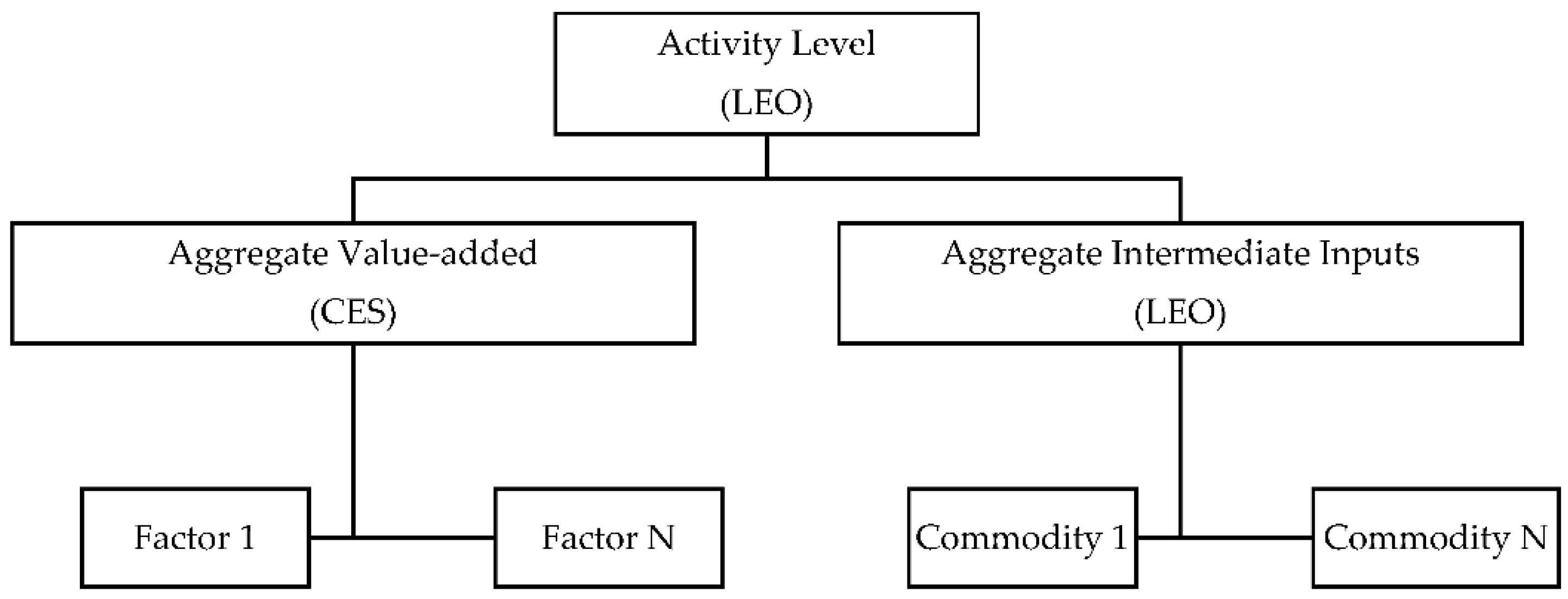
- Producers’ decisions are guided by a profit maximization goal subject to the output and input prices, and the production technology. Each producer face a two-stage production technology nest (see Figure A2). The Leontief (LEO) function combines the aggregate value-added and the aggregate intermediate input at the top of the production technology nest. The aggregate value-added nest is a composite of the primary factors of production aggregated using a constant elasticity of substitution (CES) function. The aggregate intermediate input is a composite of different intermediate commodities combined using a Leontief function.
- Every producer is allowed to produce one or more commodities that can be consumed at home (home commodities) or sold at markets (market commodities). The producers’ decision to sell market commodities in domestic or foreign markets is guided by a profit maximization goal constrained by a constant elasticity of transformation (CET) function.
- Households receive income from factors of production they own directly (e.g., labor) and indirectly (e.g., capital through enterprises), remittances from abroad, and transfers from the government. Households pay direct taxes, remit to abroad, transfer to the other household group, save, and spend on consumption. The consumption demand of households on consumption is specified by the linear expenditure system (LES). Households are allowed to consume both home commodities (valued at producer prices) and market commodities (valued at sales prices). The consumption bundle of households includes both domestic and foreign varieties of goods aggregated using a CES function.
Figure A2.
Schematic presentation of the production technology nest. Source: Authors’ illustration based on [54].
Figure A2.
Schematic presentation of the production technology nest. Source: Authors’ illustration based on [54].

The CGE model database is the 2005/06 SAM of Ethiopia [34]. We modify the original SAM into 54 total accounts that consist of 17 activity, 18 commodity, eight factor, two household, three tax, and six other accounts (enterprise, government, rest of the world, savings-investment, changes in stock inventory, and transport and trade margin). The calibration of the model to the SAM involves a specification of a production technology nest, a range of elasticities, a factor market closure, and a combination of macro closures that are common to the empirical CGE modelling for developing countries. The following are the key features of our calibration:
- The values of the elasticities are collected from the empirical literature. The values of elasticities of factor substitution increase from agricultural activities to service activities, and income elasticities of demand increase from agricultural commodities to services commodities. The elasticities of export transformation and import substitution increase with tradability of the commodities. We set the absolute value of the Frisch parameter to 2 (for rural households) and to 1.5 (for urban households).
- All factors are assumed to be fully employed. For each factor, an economy-wide wage rate is flexible to assure that the sum of factor demands is equal to the fixed (observed) quantity of factor supply. All categories of labor and land are assumed to be mobile across activities whereas livestock and capital are activity-specific. We obtain the observed employment of each labor category by activity from [39]. We use the [32] to allocate the total agricultural labor among the five agricultural activities of the modified SAM, and to compute the tropical livestock unit (TLU, a factor used only in the livestock activity). We set the average wage rate of capital factor equal to unity. Thus, the observed employment of capital per activity is represented by the payment from the activity to capital factor in the SAM.
- The combination of the macroeconomic closures is the ‘Johansen’ type [54]. For the external sector balance, the real exchange rate is flexible while the foreign saving is fixed. The government’s saving adjusts to maintain the balance between the government’s revenue and recurrent expenditure. All tax rates and real government consumption of goods and services are fixed. The saving-investment (S-I) balance closure is investment-driven.
- The consumer price index (CPI) is the numeraire of the model. All simulated changes shall be interpreted relative to this numeraire.

Table A1.
Summary of elasticities used in calibration of the CGE model.
| Elasticities | Applied for | Values |
|---|---|---|
| Elasticities of factor substitution | All activities | 0.3–2.0 |
| Elasticities of import substitution | All import goods | 0.5–2.0 |
| Elasticities of export transformation | All export goods | 0.5–2.0 |
| Income elasticities | All household consumption goods | 0.7–1.5 |
| Frisch parameter (absolute value) | Both household groups | 1.5–2.0 |
Source: Authors’ desk review. The list of references for this specific table can be obtained from the authors.
Appendix A.3. Regional Module and Projections
Due to lack of data, we simply assume that activities in each region produce a constant portion of the corresponding country-wide activity output [60]. In other words, the regional shares () are exogenous and fixed:
Accordingly, the effects of a specific CGE simulation on output of an activity in a region () is equal to the effect of the same simulation on the country-wide output of the same activity () [58,59]. For example, a 10% decrease in the economy’s aggregate sectoral output of manufacturing leads to a 10% decrease in the output of manufacturing in each region [59]:
The Ethiopia-wide sectoral output effects () are simulated by the CGE model. Then, for each of the eleven regions, the regional projections involve taking the Ethiopia-wide effects in all of the economic sectors as ‘inputs’ to compute the overall regional effects () of a specific CGE experiment:
where represents the share of industry a in region r’s region-wide value-added GDP. It captures the importance of a specific industry in region r. Since data for regional industry-wise output and region-wide GDP are not available in Ethiopia, we took remedial measures. We compute sector-wise and region-wide GDP at factor cost directly from the SAM.
- We apply a simple rule to disaggregate the Ethiopia-wide sectoral output to obtain regional sectoral output. We find the employment data to be relatively comprehensive and easy to map with the SAM. We take a regional share in Ethiopia-wide sectoral employment as proxy to a regional share in Ethiopia-wide sectoral output. Our main source of employment data, per industry, in each region is [39]. We made adjustments. We used the population and housing census [61] to control for a possible sampling bias in the labor force survey [39]. We use [32] to adjust employment among agricultural activities. We use the government expenditure on agriculture and rural development in each region [62] to compute regional shares in activity of public administration (agriculture) services (i.e., public admin. (agri.) in Table A2 below).
- We compute the sector-wise output of the 17 activities for each region based on the regional shares from the previous step. Summing the regional sector-wise outputs gives the region-wide GDP for each region.
- To check the robustness of the regional module, we apply the same procedures using employment data from [73] instead of [39]. The economic structure of many regions remain more or less. Only the case with Tigray region where the employment in manufacturing activity in [73] is lower than what is reported in [39] was an exception. Thus, the regional module based on the former increases the role of agriculture in Tigray region. There are no noticeable differences in the rest of the regions. We retain the case with data from [39] as it is also used for creating the original SAM [34].
Table A2.
Regional module (economic structure of Ethiopian regions).
| Notation | Description | ETH | Region | ||||||||||
|---|---|---|---|---|---|---|---|---|---|---|---|---|---|
| TIG | AFR | AMH | ORM | SOM | BNG | SNNP | GAM | HAR | ADD | DD | |||
| AGRAIN | Grain crops | 18 | 21 | 7 | 34 | 21 | 8 | 26 | 13 | 11 | 5 | 0 | 3 |
| ACCROP | Cash crops | 10 | 2 | 7 | 7 | 12 | 7 | 5 | 19 | 15 | 9 | 0 | 3 |
| AENSET | Enset crop | 1 | 0 | 0 | 0 | 0 | 0 | 0 | 5 | 1 | 0 | 0 | 0 |
| ALIVST | Livestock | 14 | 5 | 15 | 12 | 20 | 13 | 3 | 20 | 2 | 1 | 0 | 2 |
| AFISFOR | Fishing & forestry | 5 | 0 | 3 | 2 | 2 | 25 | 0 | 8 | 0 | 0 | 0 | 0 |
| AMINQ | Mining & quarrying | 1 | 2 | 0 | 0 | 0 | 1 | 9 | 0 | 2 | 1 | 0 | 1 |
| ACONS | Construction | 4 | 14 | 4 | 5 | 3 | 2 | 15 | 1 | 6 | 5 | 8 | 8 |
| AMAN | Manufacturing | 7 | 7 | 12 | 9 | 7 | 3 | 9 | 5 | 7 | 4 | 7 | 4 |
| ATSER | Wholesale & retail trade | 11 | 9 | 12 | 7 | 12 | 14 | 9 | 12 | 18 | 27 | 12 | 27 |
| AHSER | Hotels & restaurants | 2 | 2 | 2 | 2 | 3 | 1 | 3 | 2 | 1 | 1 | 2 | 1 |
| ATRNCOM | Transport & comm. | 5 | 3 | 8 | 3 | 3 | 6 | 1 | 2 | 8 | 10 | 19 | 22 |
| AFSER | Financial intermediaries | 2 | 1 | 5 | 1 | 1 | 2 | 1 | 1 | 3 | 3 | 6 | 4 |
| ARSER | Real estate & renting | 8 | 7 | 6 | 7 | 5 | 9 | 2 | 4 | 6 | 4 | 25 | 10 |
| APADMN | Public admin. (general) | 4 | 13 | 9 | 2 | 2 | 4 | 7 | 2 | 9 | 14 | 7 | 4 |
| APAGRI | Public admin. (agri) | 1 | 4 | 2 | 1 | 1 | 1 | 2 | 1 | 2 | 1 | 0 | 1 |
| ASSER | Social services | 4 | 5 | 5 | 4 | 4 | 3 | 6 | 3 | 7 | 13 | 7 | 5 |
| AOSER | Other services | 3 | 4 | 3 | 2 | 3 | 2 | 2 | 1 | 3 | 4 | 7 | 6 |
| TOTAL | Total GDP at factor cost | 100 | 100 | 100 | 100 | 100 | 100 | 100 | 100 | 100 | 100 | 100 | 100 |
Notes: ETH (Ethiopia), TIG (Tigray regional state), AFR (Afar regional state), AMH (Amhara regional state), ORM (Oromia regional state), SOM (Somali regional state), BNG (Benshangul-Gumuz regional state), SNNP (Southern nations, nationalities, and peoples regional state), GAM (Gambella regional state), HAR (Harari regional state), ADD (Addis Ababa city administration), and DD (Dire Dawa city council). Source: Authors’ construction.
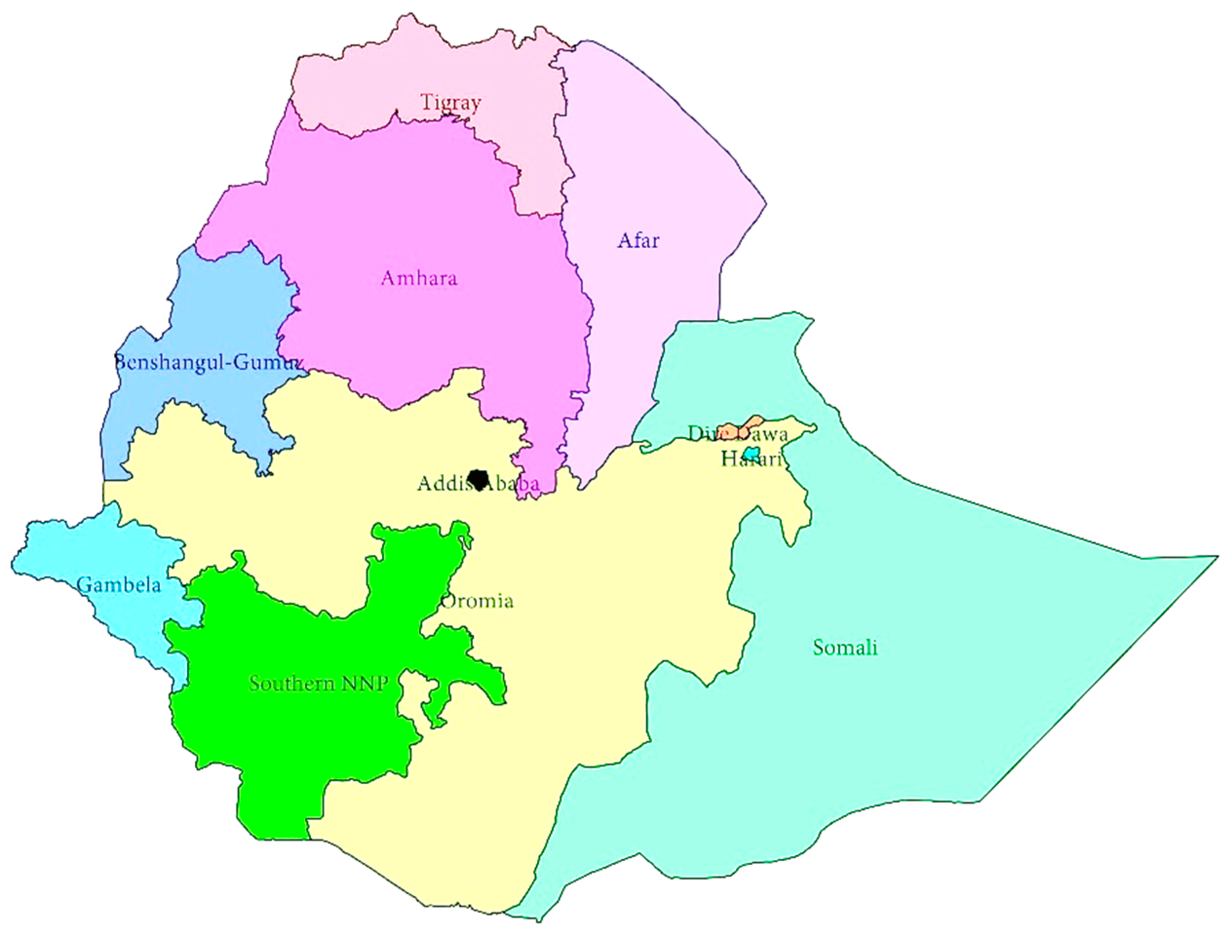
Figure A3.
Administrative units (regions) of Ethiopia.

References
- Müller, C.; Waha, K.; Bondeau, A.; Heinke, J. Hotspots of climate change impacts in sub-Saharan Africa and implications for adaptation and development. Glob. Chang. Biol. 2014, 20, 2505–2517. [Google Scholar] [CrossRef] [PubMed]
- Hertel, T.W.; Lobell, D.B. Agricultural adaptation to climate change in rich and poor countries: Current modeling practice and potential for empirical contributions. Energy Econ. 2014, 46, 562–575. [Google Scholar] [CrossRef]
- Knox, J.; Hess, T.; Daccache, A.; Wheeler, T. Climate change impacts on crop productivity in Africa and South Asia. Environ. Res. Lett. 2012, 7, 034032. [Google Scholar] [CrossRef] [Green Version]
- Schlenker, W.; Lobell, D.B. Robust negative impacts of climate change on African agriculture. Environ. Res. Lett. 2010, 5, 014010. [Google Scholar] [CrossRef] [Green Version]
- Nelson, G.C.; Rosegrant, M.W.; Koo, J.; Robertson, R.; Sulser, T.; Zhu, T.; Lee, D. The Costs of Agricultural Adaptation to Climate Change; Development and Climate Change Discussion Paper No. 4; World Bank: Washington, DC, USA, 2010. [Google Scholar]
- Adams, R.M.; Hurd, B.H.; Lenhart, S.; Leary, N. Effects of global climate change on agriculture: An interpretative review. Clim. Res. 1998, 11, 19–30. [Google Scholar] [CrossRef]
- Thornton, P.K.; van de Steeg, J.; Notenbaert, A.; Herrero, M. The impacts of climate change on livestock and livestock systems in developing countries: A review of what we know and what we need to know. Agric. Syst. 2009, 101, 113–127. [Google Scholar] [CrossRef]
- Nardone, A.; Ronchi, B.; Lacetera, N.; Ranieri, M.S.; Bernabucci, U. Effects of climate changes on animal production and sustainability of livestock systems. Livest. Sci. 2010, 130, 57–69. [Google Scholar] [CrossRef]
- Seo, S.N.; Mendelsohn, R. Measuring impacts and adaptations to climate change: A structural Ricardian model of African Livestock management. Agric. Econ. 2008, 38, 151–165. [Google Scholar] [CrossRef]
- Antle, J.M.; Capalbo, S.M. Adaptation of agricultural and food systems to climate change: An economic and policy. Appl. Econ. Perspect. Policy 2010, 32, 386–416. [Google Scholar] [CrossRef]
- Kubik, Z.; Mathilde, M. Weather shocks, agricultural production and migration: Evidence from Tanzania. J. Dev. Stud. 2016, 52, 665–680. [Google Scholar] [CrossRef]
- Mertz, O.; Mbow, C.; Reenberg, A.; Genesio, L.; Lambin, E.F.; D’haen, S.; Sandholt, I. Adaptation strategies and climate vulnerability in the Sudano-Sahelian region of West Africa. Atmos. Sci. Lett. 2011, 12, 104–108. [Google Scholar] [CrossRef] [Green Version]
- Naude, W. The determinants of migration from sub-Saharan African Countries. J. Afr. Econ. 2010, 19, 330–356. [Google Scholar] [CrossRef]
- Brown, O. Migration and Climate Change; IOM Migration Research Series, No. 31; International Organization for Migration: Geneva, Switzerland, 2008. [Google Scholar]
- McLeman, R.; Smit, B. Migration as an adaptation to climate change. Clim. Chang. 2006, 76, 31–53. [Google Scholar] [CrossRef]
- Alagidede, P.; Adu, G.; Frimpong, P.B. The effect of climate change on economic growth: Evidence from sub-Saharan Africa. Environ. Econ. Policy Stud. 2016, 18, 417–436. [Google Scholar] [CrossRef]
- Dell, M.; Jones, B.F.; Olken, B.A. Temperature shocks and economic growth: Evidence from the last half century. Am. Econ. J. Macroecon. 2012, 4, 66–95. [Google Scholar] [CrossRef] [Green Version]
- Jones, B.F.; Olken, B.A. Climate shocks and exports. Am. Econ. Rev. Pap. Proc. 2010, 100, 454–459. [Google Scholar] [CrossRef]
- Climate Change Knowledge Portal. Available online: http://data.worldbank.org/country/ethiopia (accessed on 24 September 2016).
- Conway, D.; Schipper, E.F. Adaptation to climate change in Africa: Challenges and opportunities identified from Ethiopia. Glob. Environ. Chang. 2011, 21, 227–237. [Google Scholar] [CrossRef]
- Kassie, B.T. Climate Variability and Change in Ethiopia: Exploring Impacts and Adaptation Options for Cereal Production. Ph.D. Thesis, Wageningen University, Wageningen, The Netherlands, 2014. [Google Scholar]
- Admassu, G.; Getinet, M.; Thomas, T.S.; Waithaka, M.; Kyotalimye, M. Ethiopia. In East African Agriculture and Climate Change: A Comprehensive Analysis; Waithaka, M., Nelson, G.C., Thomas, T.S., Kyotalimye, M., Eds.; International Food Policy Research Institute: Washington, DC, USA, 2013; pp. 149–182. [Google Scholar]
- Evangelista, P.; Young, N.; Burnett, J. How will climate change spatially affect agriculture production in Ethiopia? Case studies of important cereal crops. Clim. Chang. 2013, 119, 855–873. [Google Scholar] [CrossRef]
- Deressa, T.T.; Hassan, R.M. Economic impact of climate change on crop production in Ethiopia: Evidence from cross-section measures. J. Afr. Econ. 2009, 18, 529–554. [Google Scholar] [CrossRef]
- Arndt, C.; Robinson, S.; Willenbockel, D. Ethiopia’s growth prospects in a changing climate: A stochastic general equilibrium approach. Glob. Environ. Chang. 2011, 21, 701–710. [Google Scholar] [CrossRef]
- World Bank. Economics of Adaptation to Climate Change: Ethiopia; World Bank: Washington, DC, USA, 2010. [Google Scholar]
- AgMIP Tool: A GEOSHARE Tool for Aggregating Outputs from the AgMIP’s Global Gridded Crop Modeling Initiative (Ag-GRID). Available online: https://mygeohub.org/resources/agmip (accessed on 24 November 2015).
- Moss, R.H.; Edmonds, J.A.; Hibbard, K.A.; Manning, M.R.; Rose, S.; van Vuuren, D.P.; Wilbanks, T.J. The next generation of scenarios for climate change research and assessment. Nature 2010, 463, 747–756. [Google Scholar] [CrossRef] [PubMed]
- Rosenzweig, C.; Elliott, J.; Deryng, D.; Ruane, A.C.; Müller, C.; Arneth, A.; Jones, J.W. Assessing agricultural risks of climate change in the 21st century in a global gridded crop model intercomparison. Proc. Natl. Acad. Sci. USA 2010, 111, 3268–3273. [Google Scholar] [CrossRef] [PubMed] [Green Version]
- Müller, C.; Robertson, R.D. Projecting future crop productivity for global economic modeling. Agric. Econ. 2014, 45, 37–50. [Google Scholar] [CrossRef]
- Annual Agricultural Sample Survey (AgSS); Central Statistics Agency: Addis Ababa, Ethiopia, 2014. Available online: www.csa.gov.et (accessed on 15 November 2015).
- Annual Agricultural Sample Survey (AgSS); Central Statistics Agency: Addis Ababa, Ethiopia, 2006. Available online: www.csa.gov.et (accessed on 15 November 2015).
- Ethiopia’s Agricultural Sector Policy and Investment Framework: 2010–2020; Ministry of Agriculture and Rural Development (MoARD): Addis Ababa, Ethiopia, 2010.
- Input-output Table and Social Accounting Matrix; Ethiopian Development Research Institute (EDRI): Addis Ababa, Ethiopia, 2009.
- Agricultural Sample Survey Time Series Data for National and Regional Level: From 1995/96–2014/15: Report on Crop Area and Production; Central Statistics Agency: Addis Ababa, Ethiopia, 2015. Available online: www.csa.gov.et (accessed on 20 April 2016).
- Robinson, S.; Strzepek, K.; Cervigni, R. The Cost of Adapting to Climate Change in Ethiopia: Sector-Wise and Macro-Economic Estimates; ESSP II Working Paper No. 53; Ethiopia Strategic Support Program II; Ethiopian Development Research Institute (EDRI): Addis Ababa, Ethiopia, 2013. [Google Scholar]
- Weindl, I.; Lotze-Campen, H.; Popp, A.; Müller, C.; Havlík, P.; Herrero, M.; Rolinski, S. Livestock in a changing climate: Production system transitions as an adaptation strategy for agriculture. Environ. Res. Lett. 2015, 10, 094021. [Google Scholar] [CrossRef]
- National Labor Force Survey; Central Statistics Agency: Addis Ababa, Ethiopia, 2013. Available online: www.csa.gov.et (accessed on 14 December 2015).
- National Labor Force Survey; Central Statistics Agency: Addis Ababa, Ethiopia, 2005. Available online: www.csa.gov.et (accessed on 14 December 2015).
- National Labor Force Survey; Central Statistics Agency: Addis Ababa, Ethiopia, 1999. Available online: www.csa.gov.et (accessed on 14 December 2015).
- Inter-Censal Population Survey; Central Statistics Agency: Addis Ababa, Ethiopia, 2012. Available online: www.csa.gov.et (accessed on 14 December 2015).
- Gebeyehu, Z.H. Land Policy Implications in Rural-Urban Migration: The Dynamics and Determinant Factors of Rural-Urban Migration in Ethiopia. Ph.D. Thesis, Technische Universität München, Munich, Germany, 2015. [Google Scholar]
- Gray, C.; Mueller, V. Drought and population mobility in rural Ethiopia. World Dev. 2012, 40, 134–145. [Google Scholar] [CrossRef] [PubMed]
- Miheretu, B.A. Causes and Consequences of Rural-Urban Migration: The Case of Woldiya Town, North Ethiopia. Master’s Thesis, University of South Africa, Pretoria, South Africa, 2011. [Google Scholar]
- Dercon, S. Growth and shocks: Evidence from rural Ethiopia. J. Dev. Econ. 2004, 74, 309–329. [Google Scholar] [CrossRef]
- Ezra, M. Demographic response to environmental stress in drought- and famine-prone areas of northern Ethiopia. Int. J. Popul. Geogr. 2001, 7, 259–279. [Google Scholar] [CrossRef]
- Ezra, M.; Kiros, G.E. Rural out-migration in the drought prone areas of Ethiopia: A multilevel analysis. Int. Migr. Rev. 2001, 35, 749–771. [Google Scholar] [CrossRef] [PubMed]
- National Bank Annual Report 2014–2015; National Bank of Ethiopia: Addis Ababa, Ethiopia, 2016. Available online: http://www.nbe.gov.et/publications/annualreport.html (accessed on 12 January 2017).
- Growth and Transformation Plan II: 2015/16–2019/20; National Planning Commission of Ethiopia: Addis Ababa, Ethiopia, 2016.
- Universal Rural Road Access Program; Ethiopian Roads Authority: Addis Ababa, Ethiopia, 2010. Available online: http://www.era.gov.et/documents/10157/72095/UNIVERSAL+RURAL+ROAD+ACCESS+PROGRAM.pdf (accessed on 24 April 2015).
- Yalew, A.W.; Hirte, G.; Lotze-Campen, H.; Tscharaktschiew, S. Economic Effects of Climate Change in Developing Countries: Economy-Wide and Regional Analysis for Ethiopia; Working Paper 10/17; CEPIE: Dresden, Germany, 2017. [Google Scholar]
- Gabre-Madhin, E.Z. Market Institutions, Transaction Costs, and Social Capital in the Ethiopian Grain Market; Research Report No. 124; International Food Policy Research Institute: Washington, DC, USA, 2001. [Google Scholar]
- Stifel, D.; Minten, B.; Koru, B. Economic benefits of rural feeder roads: Evidence from Ethiopia. J. Dev. Stud. 2016, 52, 1335–1356. [Google Scholar] [CrossRef]
- Lofgren, H.; Harris, L.R.; Robinson, S. A Standard Computable General Equilibrium (CGE) Model in GAMS; Microcomputers in Policy Research No. 5; International Food Policy Research Institute: Washington, DC, USA, 2002; Available online: www.ifpri.org/publication/standard-computable-general-equilibrium-cge-model-gams-0 (accessed on 10 July 2014).
- Robinson, S.; Willenbockel, D.; Strzepek, K. A dynamic general equilibrium analysis of adaptation to climate change in Ethiopia. Rev. Dev. Econ. 2012, 16, 489–502. [Google Scholar] [CrossRef]
- Pielke, R. Mistreatment of the economic impacts of extreme events in the Stern Review Report on the Economics of Climate Change. Glob. Environ. Chang. 2007, 17, 302–310. [Google Scholar] [CrossRef] [Green Version]
- Yalew, A.W.; Hirte, G.; Lotze-Campen, H.; Tscharaktschiew, S. General Equilibrium Effects of Public Adaptation in Agriculture in LDCs: Evidence from Ethiopia; Working Paper 11/17; CEPIE: Dresden, Germany, 2017. [Google Scholar]
- Higgs, P.J.; Parmenter, B.R.; Rimmer, R.J. A hybrid top-down, bottom-up regional computable general equilibrium model. Int. Reg. Sci. Rev. 1988, 11, 317–328. [Google Scholar] [CrossRef]
- Dixon, P.B.; Parmenter, B.R.; Sutton, J.; Vincent, D.P. ORANI: A Multisectoral Model of the Australian Economy; North-Holland Publishing Co.: Amsterdam, The Netherlands, 1982. [Google Scholar]
- Naqvi, F.; Peter, M.W. A multiregional, multisectoral model of the Australian economy with an illustrative application. Aust. Econ. Pap. 1996, 35, 94–113. [Google Scholar] [CrossRef]
- Population and Housing Census (PHC); Central Statistical Agency: Addis Ababa, Ethiopia, 2007. Available online: www.csa.gov.et (accessed on 24 September 2018).
- Quarterly Government Finance: National and Regional Budgets; Ministry of Finance and Economic Development (MoFED): Addis Ababa, Ethiopia, 2015.
- Wondimagegnhu, B.A. Staying or leaving? Analyzing the rationality of rural-urban migration associated with farm income of staying households: A case study from Southern Ethiopia. Adv. Agric. 2015. [Google Scholar] [CrossRef]
- De Brauw, A. Migration, Youth, and Agricultural Productivity in Ethiopia. 2014. Available online: http://ageconsearch.umn.edu//handle/189684 (accessed on 24 September 2016).
- De Boer, P.; Missaglia, M. Estimation of Income Elasticities and Their Use in a CGE Model for Palestine; Repot No. 12; Econometric Institute, Erasmus University Rotterdam: Rotterdam, The Netherlands, 2006; Available online: http://repub.eur.nl/pub/7753 (accessed on 15 January 2016).
- Von Braun, J. A Policy Agenda for Famine Prevention in Africa; Food Policy Statement No. 13; International Food Policy Research Institute: Washington, DC, USA, 1991. [Google Scholar]
- Growth and Transformation Plan: 2010/11–2014/15; Ministry of Finance and Economic Development (MoFED): Addis Ababa, Ethiopia, 2010.
- Dorosh, P.; Thurlow, J. Urbanization and Economic Transformation: A CGE Analysis for Ethiopia; ESSP II Working Paper No. 14; Ethiopia Strategy Support Program II; Ethiopian Development Research Institute (EDRI): Addis Ababa, Ethiopia, 2011. [Google Scholar]
- Fankhauser, S.; Schmidt-Traub, G. From adaptation to climate-resilient development: The costs of climate-proofing the millennium development goals in Africa. Clim. Dev. 2011, 3, 94–113. [Google Scholar] [CrossRef]
- Henderson, J.V.; Storeygard, A.; Deichmann, W. Has climate change driven urbanization in Africa? J. Dev. Econ. 2017, 124, 60–82. [Google Scholar] [CrossRef] [PubMed] [Green Version]
- Millner, A.; Dietz, S. Adaptation to climate change and economic growth in developing Countries. Environ. Dev. Econ. 2015, 20, 380–406. [Google Scholar] [CrossRef]
- Mendelsohn, R. The economics of adaptation to climate change in developing Countries. Clim. Chang. Econ. 2012, 3, 1250006. [Google Scholar] [CrossRef]
- Household Income, Consumption, and Expenditure Survey (HICES); Central Statistics Agency: Addis Ababa, Ethiopia, 2005. Available online: www.csa.gov.et (accessed on 14 December 2015).
Figure 1.
The effects of climate change on households’ welfare. Source: CGE simulations.

Figure 2.
Effects of climate change on regional value-added GDP. Source: Regional projections.

Figure 3.
Macroeconomic effects of climate change with structural change. Source: CGE simulations.

Figure 4.
The effects of climate change on total real private consumption. Source: CGE simulations.

Table 1.
Summary of CGE simulations.
| Simulation | Description |
|---|---|
| LPJmL-P | −10% and −2% productivity effects on grain and livestock activities, respectively |
| EPIC-P | −26% and −5% productivity effects on grain and livestock activities, respectively |
| LPJmL-M3 | 0.5 million workers migrating from FLAB0 to FLAB3, corresponding to LPJmL scenario |
| EPIC-M3 | 1 million workers migrating from FLAB0 to FLAB3, corresponding to EPIC scenario |
| LPJmL-PM3 | LPJmL-P and LPJmL-M (productivity plus migration effects) |
| EPIC-PM3 | EPIC-P and EPIC-M (productivity plus migration effects) |
| EPIC-PM4 | EPIC-P and 1 million labor moving from FLAB0 to FLAB4 |
| EPIC-PM2 | EPIC-P and 1 million labor moving from FLAB0 to FLAB2 |
| EPIC-PM1 | EPIC-P and 1 million labor moving from FLAB0 to FLAB1 |
| EPIC-PL0 | EPIC-P and 0.5 million extra labor force allocated to FLAB0 |
| EPIC-PL3 | EPIC-P and 0.5 million extra labor force allocated to FLAB3 |
| EPIC-PL4 | EPIC-P and 0.5 million extra labor force allocated to FLAB4 |
| EPIC-PL2 | EPIC-P and 0.5 million extra labor force allocated to FLAB2 |
| EPIC-PL1 | EPIC-P and 0.5 million extra labor force allocated to FLAB1 |
| EPIC-PTC | EPIC-P and 10% decline in marketing margins |
| EPIC-PM3TC | EPIC-PM3 and 10% decline in marketing margins |
Table 2.
Sector-wise effects of climate change.
| Activity | Simulations (% Change) | |||||
|---|---|---|---|---|---|---|
| LPJmL-P | EPIC-P | LPJmL-M3 | EPIC-M3 | LPJmL-PM3 | EPIC-PM3 | |
| Grain crops | −9.3 | −24 | −1.7 | −3.4 | −10.8 | −25.6 |
| Cash crops | −3.8 | −13.1 | −1.5 | −3.1 | −5.5 | −15.7 |
| Enset crop | −3.4 | −10.4 | −0.8 | −1.7 | −4.2 | −11.6 |
| Livestock Production | −4.0 | −11.4 | −1.3 | −2.7 | −5.3 | −13.6 |
| Fishing & forestry | −2.5 | −8.1 | −1.1 | −2.2 | −3.6 | −10.0 |
| Mining & quarrying | 0.8 | 2.2 | 1.6 | 3.0 | 2.4 | 5.1 |
| Construction | 0.0 | −0.1 | 0.0 | 0.0 | 0.0 | 0.0 |
| Manufacturing | 2.5 | 7.0 | 3.5 | 6.7 | 6.0 | 13.2 |
| Wholesale & retail trade | −1.6 | −5.0 | 0.0 | 0.0 | −1.6 | −4.8 |
| Hotels & restaurants | −0.8 | −3.2 | 0.5 | 0.8 | −0.4 | −2.6 |
| Transport & comm. | 1.2 | 4.0 | 0.7 | 1.4 | 2.0 | 5.6 |
| Financial intermediaries | 0.2 | 0.5 | 0.8 | 1.4 | 0.9 | 1.9 |
| Real estate & renting | 0.0 | 0.0 | 0.1 | 0.2 | 0.1 | 0.2 |
| Public admin. (general) | 0.0 | 0.0 | 0.0 | 0.0 | 0.0 | 0.0 |
| Public admin. (agriculture) | 0.0 | 0.0 | 0.0 | 0.0 | 0.0 | 0.0 |
| Social services | 0.1 | 0.1 | 0.3 | 0.6 | 0.4 | 0.7 |
| Other services | 1.1 | 3.3 | 5.1 | 9.8 | 6.2 | 13.5 |
| Total GDP at factor cost | −2.7 | −7.6 | −0.2 | −0.5 | −2.9 | −7.6 |
Source: CGE simulations.
© 2018 by the authors. Licensee MDPI, Basel, Switzerland. This article is an open access article distributed under the terms and conditions of the Creative Commons Attribution (CC BY) license (http://creativecommons.org/licenses/by/4.0/).
Share and Cite
MDPI and ACS Style
Yalew, A.W.; Hirte, G.; Lotze-Campen, H.; Tscharaktschiew, S. Climate Change, Agriculture, and Economic Development in Ethiopia. Sustainability 2018, 10, 3464. https://doi.org/10.3390/su10103464
AMA Style
Yalew AW, Hirte G, Lotze-Campen H, Tscharaktschiew S. Climate Change, Agriculture, and Economic Development in Ethiopia. Sustainability. 2018; 10(10):3464. https://doi.org/10.3390/su10103464
Chicago/Turabian StyleYalew, Amsalu Woldie, Georg Hirte, Hermann Lotze-Campen, and Stefan Tscharaktschiew. 2018. "Climate Change, Agriculture, and Economic Development in Ethiopia" Sustainability 10, no. 10: 3464. https://doi.org/10.3390/su10103464
Note that from the first issue of 2016, this journal uses article numbers instead of page numbers. See further details here.