Genetic Algorithm-Optimized Long Short-Term Memory Network for Stock Market Prediction

Ewha School of Business, Ewha Womans University, 52 Ewhayeodae-gil, Seodaemun-gu, Seoul 03760, Korea
*
Author to whom correspondence should be addressed.
Sustainability 2018, 10(10), 3765; https://doi.org/10.3390/su10103765
Submission received: 28 September 2018
/
Revised: 16 October 2018
/
Accepted: 16 October 2018
/
Published: 18 October 2018
(This article belongs to the Special Issue Expert Systems: Applications of Business Intelligence in Big Data Environments)
Abstract
:With recent advances in computing technology, massive amounts of data and information are being constantly accumulated. Especially in the field of finance, we have great opportunities to create useful insights by analyzing that information, because the financial market produces a tremendous amount of real-time data, including transaction records. Accordingly, this study intends to develop a novel stock market prediction model using the available financial data. We adopt deep learning technique because of its excellent learning ability from the massive dataset. In this study, we propose a hybrid approach integrating long short-term memory (LSTM) network and genetic algorithm (GA). Heretofore, trial and error based on heuristics is commonly used to estimate the time window size and architectural factors of LSTM network. This research investigates the temporal property of stock market data by suggesting a systematic method to determine the time window size and topology for the LSTM network using GA. To evaluate the proposed hybrid approach, we have chosen daily Korea Stock Price Index (KOSPI) data. The experimental result demonstrates that the hybrid model of LSTM network and GA outperforms the benchmark model.
1. Introduction
With recent advances in computing technology, massive amounts of data and information are being constantly accumulated. Big data is being used as a key mechanism to support the innovation of artificial intelligence (AI) techniques, which are undergoing rapid development in recent years, and it is expected to play an important role in improving social and environmental sustainability. This study adopts big data and AI techniques in the field of finance, in order to manage the potential risks of financial market and help achieve socioeconomic sustainability.
In the field of finance, we have great opportunities to create useful insights by analyzing this information, because the financial market produces a tremendous amount of real-time data, including transaction records. Accordingly, this study intends to develop a novel stock market prediction model using the available financial data. We adopt a deep learning technique, since one of the main advantages of this technique is the excellent learning ability from massive datasets.
Stock market predictions have an important role, since they can significantly impact the global economy. Due to of its functional importance, analyzing stock market volatility has become a major research issue in various areas, including finance, statistics, and mathematics [1]. However, most stock indices behave very similarly to a random walk, because the financial time series data is noisy and non-stationary in nature [2]. Undoubtedly, it is very difficult to predict the stock market, since the volatility is too large to be captured in a model [3].
Despite these difficulties, there has been a constant desire to develop a reliable stock market prediction model [4]. Several approaches, in recent decades, have been made to forecast stock markets using statistics and soft computing skills. Most early studies tend to employ statistical methods, but these approaches have limitations when applied to the complicated real-world financial data, due to many statistical assumptions, such as linearity and normality [5]. Accordingly, various machine learning techniques, including artificial neural network (ANN) and support vector machine (SVM), that can reflect nonlinearity and complex characteristics of financial time series, have started being applied to stock market prediction. These approaches have provided prominent skills in predicting the chaotic environments of stock markets by capturing their nonlinear and unstructured nature [6,7].
In recent years, there have been increasing attempts to apply deep learning techniques to stock market prediction. Deep learning is a generic term for an ANN with multiple hidden layers between the input and output layers. They have been attracting significant attention for their excellent predictability in image classification and natural language processing (NLP). Deep belief network (DBN), convolution neural network (CNN), and recurrent neural network (RNN) are representative methodologies of deep learning. In particular, RNN is mainly used for time series analysis, because it has feedback connections inside the network that allow past information to persist, and time series and nonlinear prediction capabilities. Conventional ANNs do not take the “temporal effects” of past significant events into account [8]. The temporal representation capabilities of RNN have advantages in tasks that process sequential data, such as financial predictions, natural language processing, and speech recognition [9]. Traditional neural networks cannot handle this type of data effectively, which is one of their major weaknesses. This study intends to overcome this limitation by applying RNN to stock market predictions. We adopt long short-term memory (LSTM) units for sequence learning of financial time series. LSTM is a state-of-the-art unit of RNN, and RNN composed of LSTM units is generally referred to as “LSTM networks”. They are one of the most advanced deep learning algorithms, but less commonly applied to the area of financial prediction, yet inherently appropriate for this domain.
Despite LSTM network being used as a powerful tool in time series and pattern recognition problems, there are several drawbacks in using an LSTM network. First, neural network models, including LSTM network, suffer from a lack of ability to explain the final decision that models acquire. The neural network models have a highly complex computational process, which can achieve a prominent solution for the target problem to be solved. However, they are not able to provide specific explanations for their prediction results. To avoid this problem, Shin and Lee (2002) proposed a hybrid approach of integrating genetic algorithm (GA) and ANN, and extracted rules from the bankruptcy prediction model [10]. Castro et al. (2002) investigated fuzzy rules from an ANN to provide an interpretation of classification decisions that were made by neural network model [11]. Second, like other neural network models, LSTM network has numerous parameters that must be modified by the researcher, such as the number of layers, neurons per layer, and number of time lags. However, time and computation limitations make it impossible to sweep through a parameter space and find the optimal set of parameters. In previous research, the determination of those control parameters has heavily depended on the experience of researchers. In spite of its importance, there is little research on investigation of optimal parameters for LSTM networks. Accordingly, we comprehensively handle these aspects of LSTM models that significantly affect the performance of stock market prediction models. This study proposes a hybrid model that integrates LSTM network with a GA to search for a suitable model for prediction of the next-day index of the stock market. We focus on the optimization of architectural factors related to the detection of temporal patterns of a given dataset, such as the size of time window and number of LSTM units in hidden layers. GA is used to determine the size of the trends to be considered in a model, and simultaneously investigate the optimal topology for hidden layers of LSTM network. Especially, detecting the appropriate size for the time window that can contain the context of the dataset is a crucial task when designing the LSTM network. If the time window is too small, significant signals may be missed, whereas if the size of time window is too big, unsuitable information may act as noise. Regarding the investigation of the time window of RNN, many studies have suggested general approaches based on statistical methods or trial and error, along with various heuristics. We apply GA technique to obtain the best solution and optimize the prediction efficacy [12]. To the best of our knowledge, most research on LSTM network does not take this aspect into account. We tested our method on the Korea Composite Stock Price Index (KOSPI) for 2000–2016, and found that it was more predictable than other methods.
The remainder of this paper is organized as follows: Section 2 provides a brief overview of the theoretical literature. Section 3 describes the methodologies that are used in this study, and introduces the hybrid model of LSTM network and GA. Section 4 describes data and variables that are used in this study. Section 5 presents the experimental results and compares the proposed method to a benchmark model. Section 6 summarizes the findings and provides suggestions for further research.
2. Related Works
2.1. Stock Market Prediction
Stock market forecasting is a known challenging task, since it is characterized by being non-stationary and with a high degree of uncertainty [2]. Stock market prediction has been studied for decades, although the efficient market hypothesis (EMH) asserts that price changes in capital market can occur independently; in addition, several empirical studies have demonstrated that stock market predictions are possible, to some extent [4,13,14]. EMH can be divided into three types (weak, semi-strong, and strong) according to the level of reflection of market information. Among three types of EMH exist, this study assumes weak EMH, which only concerns past market trading data [15].
Previous studies usually employed statistical and machine learning techniques to forecast future financial values. Traditional stock market prediction techniques, based on statistical methods, are generated via a linear process [12]. Statistical analysis based on historical stock data, such as the autoregressive integrated moving average model (ARIMA), the autoregressive conditional heteroscedasticity (ARCH) model, and the generalized autoregressive conditional heteroscedasticity (GARCH) model, has been widely used to make predictions about the financial market [16,17,18,19]. However, prediction systems based on statistical methods do not perform well, and have their own limitations because they require more historical data to meet statistical assumptions, such as normality postulates [20].
Since stock markets are regarded as nonlinear and non-parametric dynamic systems [2], more flexible methods that can learn complex dimensionality are essential to improve the prediction performance. Machine learning techniques have strong advantages in that respect, because they can extract nonlinear relationships between data without prior knowledge of the input data [3]. These techniques have been widely adopted, with relative success in making stock market predictions [21]. Among them, ANN and SVM are the most popular techniques for forecasting financial time series, since they can investigate the noisy behavior of data without making any statistical restrictions [4]. Empirical results show that machine learning techniques produce outstanding performance as compared with statistical models [7,22], since they have a better ability to learn the hidden relationships among market factors and capture the complex patterns in data [23].
Saad et al. (1998) compared three neural network models, time delay, recurrent, and probabilistic neural networks, and employed training methods of conjugate gradient and multi-stream extended Kalman filter for time delay neural network (TDNN) and RNN for stock trend prediction [9]. RNN showed the best performance among other models. Chen et al. (2005) utilized the neural network, TS fuzzy system and hierarchical fuzzy system to verify the efficacy of the hybrid model, and various parameters of each models were optimized by one of the search algorithms, the particle swarm optimization (PSO) algorithm [24]. Yu et al. (2014) employed SVM to construct stock selection system and applied principal component analysis (PCA) to get low dimensional and informative financial time series [25]. The experimental result showed that the return of stocks selected by PCA–SVM were apparently superior to other benchmarks. Chen and Hao (2017) proposed the hybrid framework to predict the stock market indices with feature weighted SVM and feature weighted K-nearest neighbor [26]. They used information gain to consider the influence of each feature and made it possible to take into account the relative importance of each feature.
Recently, with the outstanding performance in various classification problems [27,28], there have been attempts to apply deep learning techniques to stock market prediction. Deep learning techniques have achieved remarkable success in numerous prediction tasks, since they can extract useful features automatically during the learning process [29,30].
Chong et al. (2017) predicted future market trend by examining the effect of three unsupervised feature extraction methods (PCA, auto encoder, and restricted Boltzmann machine (RBM)) on the deep learning network [21]. Sezer et al. (2017) proposed a stock trading system based on deep neural network for buy–sell–hold predictions [31]. GA was used to optimize the technical analysis parameters and create the buy–sell point of the system.
There have also been some approaches to integrate qualitative information with deep learning techniques for stock market forecasting. Yoshihara et al. (2014) exploited the textual information as input variable and predicted market trends based on RNN model combined with restricted Boltzmann machine (RBM) to investigate the temporal effects of past events [8]. Ding et al. (2015) proposed an event-driven stock market prediction system [32]. The events were obtained from the news text, and deep CNN was exploited for the examining the long-term and short-term influences of extracted events on S&P 500 index and individual stock movements. Table 1 presents a summary of recent stock market prediction studies.
2.2. RNN for Time Series Prediction
Most ANNs, including multi-layer perceptron (MLP) can only learn spatial patterns from time independent inputs and outputs [5]. RNN provides advantages over traditional ANN because the “memory feature” of RNN can be employed to elicit temporal patterns in data. RNN has been used for time series analyses, due to its useful characteristics. In recent years, with the significant advance in deep learning techniques, RNN is actively applied to various tasks, such as natural language processing, speech recognition, and computer vision, that deal with sequential data [38,39]. In addition, several existing studies, using RNN including LSTM networks, achieved satisfactory performance in the financial time series forecasting problem.
Lin et al. (2009) predicted the closing price of the following trading day by utilizing one variant of RNN, echo state networks (ESN). They chose an initial transient by using Hurst exponent, and select subseries with the greatest capability of forecasting during training [6]. Wei and Cheng (2012) proposed a hybrid method using a synthesis feature selection to detect crucial technical indicators for stock market prediction [20]. They exploited the stepwise regression and decision tree to reduce the dimension of financial data. The experimental result showed the superiority of the proposed model. Dixon (2017) applied RNN to high frequency trading, classifying the movements of short-term price from limit order books of financial futures to predicting the price flip of the next event [40]. Fischer and Krauss (2018) deployed LSTM networks to forecast the directional movement of constituent stocks of the S&P 500 from 1992 to 2015 [41]. They compared the simulation result with memory-free classifiers, such as random forest (RF), deep neural network (DNN), and logistic regression. The LSTM model outperformed the other comparative models by a very clear margin, and they found that the LSTM network is suitable for the financial domain.
Furthermore, studies that integrate RNN and search algorithms have been conducted. Cai et al. (2007) combined global search algorithm PSO and evolutionary algorithm (EA) with RNN to estimate missing values in time series data [42]. Hsieh et al. (2011) suggested an integrated system with a combination of an artificial bee colony (ABC) algorithm and RNN for stock market prediction [12]. They applied ABC to optimize the connection weight of RNN, and utilized the wavelet transform to decompose the market data, along with removing the noise. Rather et al. (2015) presented an integrated model which was comprised of RNN and two linear models, including ARIMA and exponential smoothing, to predict stock returns, and the optimal weight of RNN is produced by GA [43].
RNN has highly sensitive network parameters that can affect its performance, such as the number of hidden neurons, the depth of a network, and the size of time window. Determining the time window size is particularly important, because it defines the shape of the input variables entered into the RNN, and the degree of past information to be considered. Trial and error based on heuristics is commonly used to estimate the time window size of RNN. Meanwhile, various statistical or mathematical techniques, such as autocorrelation function (ACF), rescaled range analysis (R/S analysis), and information theory, can be applied to determine the appropriate time lag for time series analysis. ACF presents the degree of autocorrelation as time progresses [5]. It represents the covariance and correlation coefficient between time points in sequential data, and investigates the pattern of seasonality. The R/S analysis is similar to ACF that is used as a measure of the long-term memory of time series [6]. Information theory is one of the quantification methods which can search the length of dimension that can lead the time series data in a statistically significant manner. Zhang et al. (2017) adopted concepts of mutual information of information theory to specify the time shift of the input variable [44]. However, most studies on RNN still follow the experience rather than systematic approaches, and the literature remains limited.
3. Methodology
3.1. Long Short-Term Memory (LSTM) Network
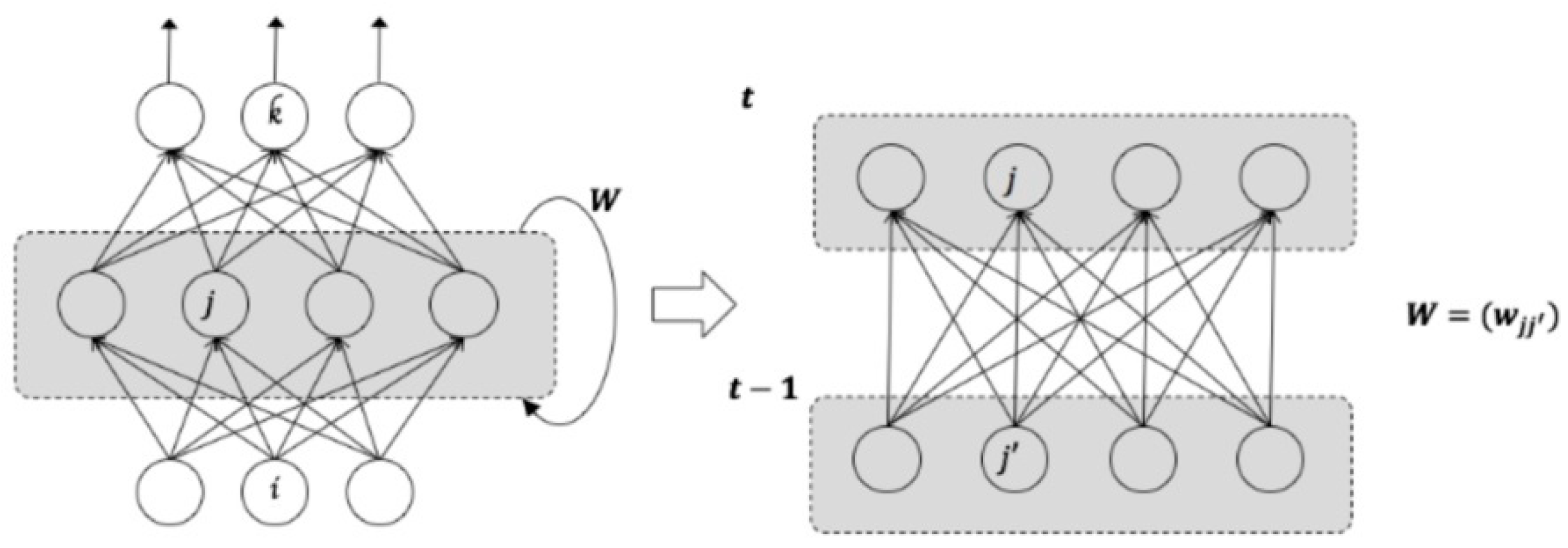
LSTM network is a type of deep RNN model composed of LSTM units. As discussed earlier, RNN is a deep learning network with internal feedback between neurons. These internal feedbacks enable the memorization of significant past events and incorporate past experience. Unlike a traditional fully connected feedforward network, RNN shares parameters across all the parts of a model, so it can be generalized to sequence lengths that have not been seen during training. Figure 1 presents an example of RNN architecture that produces an output at every time step, and has recurrent connections among hidden neurons [45].
The RNN has weight matrices that connects the input-to-hidden weight matrix , that connects hidden-to-hidden, and a weight matrix , that connects hidden-to-output. Forward propagation proceeds by defining the initial state of the hidden unit . Then, for each time step from , we apply the following update equations. The input value of hidden neuron at time is given as
where is the weight between input neuron and hidden neuron , and is input value at time . denotes the weight between hidden neuron and , and is output value of hidden neuron at time .
The transfer function of hidden neuron is named , and the output of hidden neuron is expressed as
Finally, the output value of the hidden layer is fed into output neuron , and the output value of output layer is given as
where is the weight between hidden and output neurons.
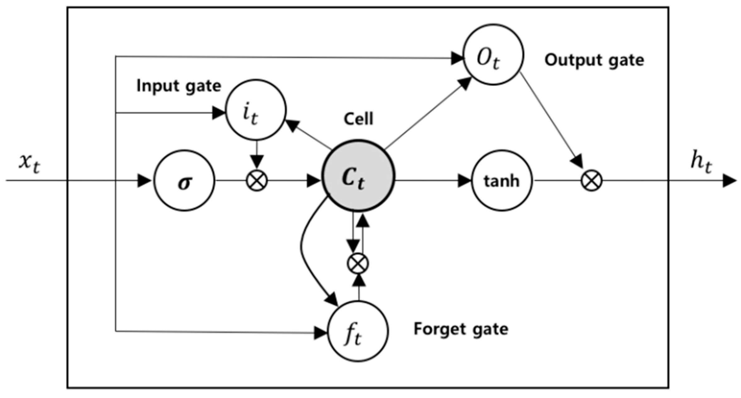
However, RNN has difficulty in learning long time-dependencies that are more than a few time steps in length [46]. As the number of time steps to consider increases, information from the past events exponentially disappears. LSTM is proposed as a way to overcome the long-term dependency problem. LSTM networks can contain past information of more than 1000 time steps. LSTM can scale to much longer sequences than simple RNN, overcoming the intrinsic drawbacks of simple RNN, i.e., vanishing and exploding gradients. Today, LSTM is widely used in many sequential modeling tasks, including speech recognition, motion detection, and natural language processing [47]. The LSTM block diagram is depicted in Figure 2.
The LSTM block contains memory cell and three multiplicative gating units; an input, an output, and a forget gate. There are recurrent connections between the cells, and each gate provides continuous operations for the cells. The cell is responsible for conveying “state” values over arbitrary time intervals, and each gate conducts write, read, and reset operations for the cells [45,46,47].
The computation process within an LSTM block is as follows. The input value can only be preserved in the state of the cell if the input gate permits it. The input value of and the candidate value of the memory cells, , at time step, t, is calculated as follows:
where , , represent the weight matrices and bias, respectively.
The weight of the state unit is managed by the forget gate and the value of forget gate is computed as
Through this process, the new state of memory cell is updated as
With the new state of memory cell, the output value of the gate is calculated as follows:
The final output value of cell is defined as
The output of the cell can be blocked by the output gate, and all gates use sigmoidal nonlinearity, and the state unit can perform as an extra input to other gating units [45,46,47]. Through this process, the LSTM architecture can solve the problem of long-term dependencies at small computational costs [48].
3.2. Genetic Algorithm (GA)
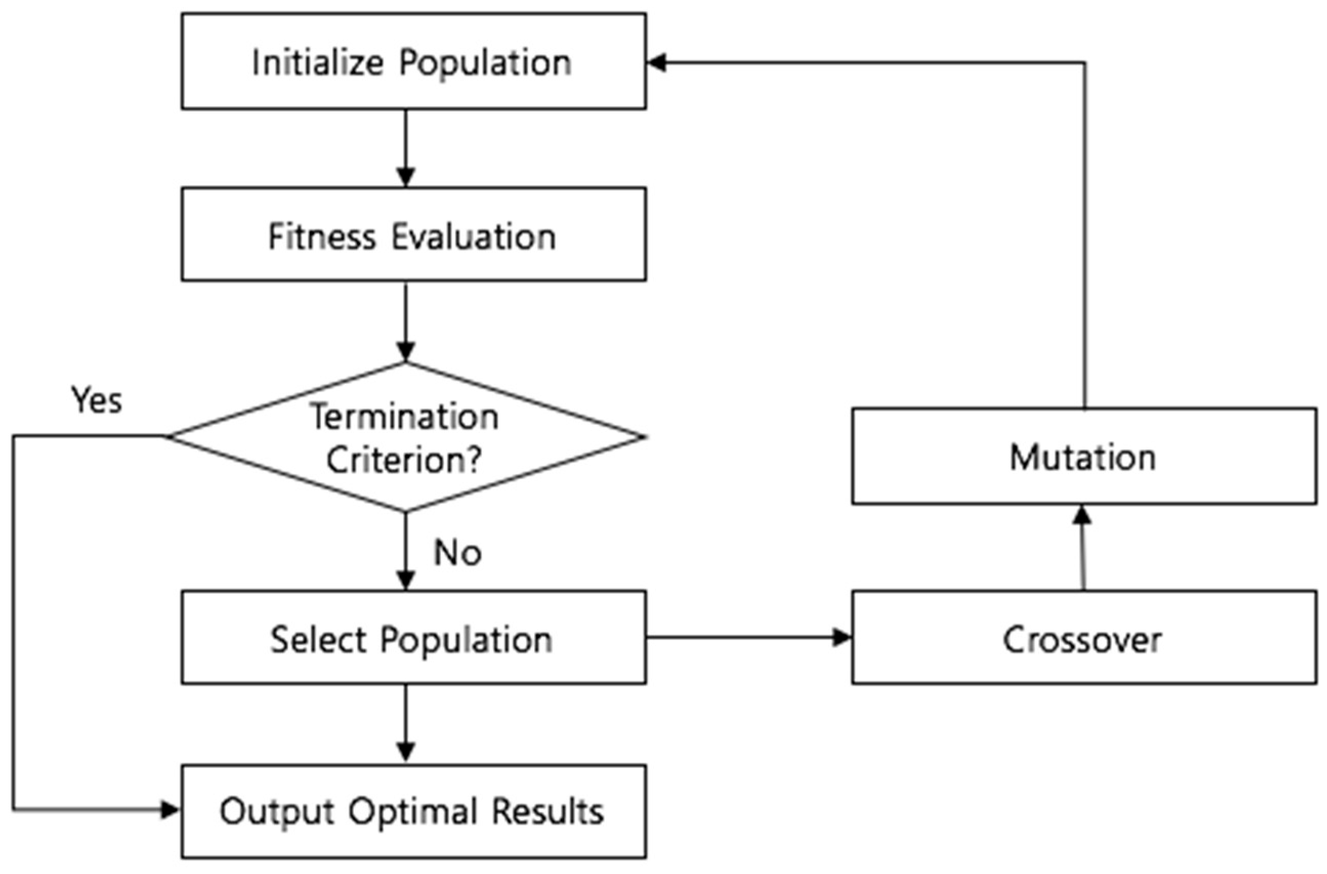
GA is metaheuristic and stochastic optimization algorithm inspired by the process of natural evolution [49]. They are widely used to find near-optimal solutions to optimization problems with large search spaces. The process of GA includes operators that imitate natural genetic and evolutionary principles, such as crossover and mutation. The major feature of GA is the population of “chromosomes”. Each chromosome acts as a potential solution to a target problem, and is usually expressed in the form of binary strings. These chromosomes are generated randomly, and the one that provides the better solution gets more chance to reproduce [15].
Processing the GA can be divided into six stages: initialization, fitness calculation, termination condition check, selection, crossover, and mutation, as shown in Figure 3 [50]. In the initialization stage, a chromosome in the search space is arbitrarily selected, and then the fitness of each selected chromosome is calculated in accordance with the predefined fitness function. The fitness function is a concept used to numerically encode a chromosome’s performance [5]. In optimization algorithms, such as GA, the definition of a fitness function is a crucial factor that affects the performance. Through the process of calculating the fitness for the fitness function, only solutions with excellent performance are preserved for further reproduction processes. Some chromosomes are selected several times through the selection process, and chromosomes that disappear without selection are generated because they are chosen stochastically according to the adaptability of fitness function. That is, the chromosomes with prominent performance have a higher probability of being inherited by the next generation. Selected superior chromosomes produce offspring by interchanging corresponding parts of the string and changing gene combinations. The crossover process leads to new solutions being created from existing ones. In the mutation process, one of the chromosomes is selected to change one randomly chosen bit. The aim of this process is to introduce diversity and novelty into the solution pool by arbitrarily swapping or turning off solution bits. The crossover process has the limitation in that completely new information cannot be generated. However, these limitations can be overcome by the mutation operation by changing corresponding bits to completely new values.
The newly generated chromosome through selection, crossover, and mutation processes calculates the fitness to the model, and verifies the termination criteria. The standard procedure of GA is over when the termination criteria have been satisfied. If some termination criteria are not satisfied, the selection, crossover, and mutation processes are repeated, to generate a superior chromosome with higher performance. In this study, chromosomes are represented as binary arrays and the mean squared error (MSE) of the prediction model is acting as the fitness value.
3.3. A Hybrid Approach to Optimization in LSTM Network with GA
Evolutionary algorithms, mostly GA, have been widely applied to neural network models, such as MLP and RNN, and used in various hybrid approaches for financial time series forecasting to optimize technical analysis or train the neural network [23,36]. Muhammad and King (1997) exploited evolutionary fuzzy networks in the foreign exchange market forecasting [51], and Kai and Wenhua (1997) proposed an ANN model trained with GA to predict the stock price [52]. Kim and Han (2000) optimized the connection weights between layers and conducted the feature discretization with GA, reducing the dimensionality of feature space [23]. Kim et al. (2006) also predicted the stock index using a GA-based multiple classifier combination technique to incorporate classifiers that stem from machine learning, experts, and users [53]. Meanwhile, combining optimized size of time window with LSTM networks in time series forecasting has not been studied extensively.
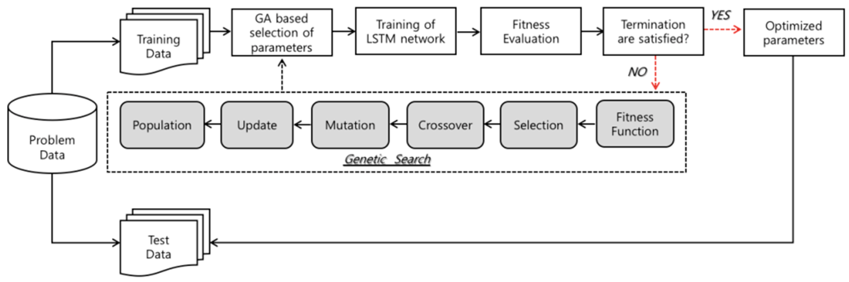
In this study, we propose a hybrid approach of LSTM network integrating GA to find the customized time window and number of LSTM units for financial time series prediction. Since LSTM network uses past information during the learning process, a suitably chosen time window plays an important role in the promising performance. If the window is too small, the model will neglect important information, while, if the window is too large, the model will be overfitted on the training data. Figure 4 depicts the flowchart of the model proposed in our work.
This study consists of two stages, which are as follows. The first stage of the experiment involves designing the appropriate network parameters for the LSTM network. We use a LSTM network with sequential input layer followed by two hidden layers, and optimal number of hidden neurons in each hidden layer is investigated by GA. In LSTM–RNN model, the hyperbolic tangent function is utilized as an activation function of the input nodes and hidden nodes. The hyperbolic tangent function is a scaled sigmoid function, and returns input value into a range between −1 and 1. The activation function of output node is designated as a linear function, since our goal is the prediction of closing price of the next day which can be formulated as a problem of regression. Initial weights of network are set as random values, and the network weight is adjusted by using a gradient-based “Adam” optimizer, which is famous for its simplicity, straightforwardness, and computational efficiency. The method is appropriate for problems which have large data and parameters, and also has strength in dealing with non-stationary problems with very noisy and sparse gradients [54].
As described above, we employ one of the evolutionary search algorithms, GA, to investigate the optimal size of time windows and architectural factors of LSTM network. In the second stage, various sizes of time windows and different numbers of LSTM units of each hidden layer are applied to evaluate the fitness of GA. The populations that are composed with possible solutions are initialized with random values, before the genetic operators start to explore the search space. The chromosomes used in this study are encoded in binary bits that represent the size of the time window and number of LSTM cells. Based on the population, the selection and recombination operators begin to search for the superior solution. The solutions are evaluated by predefined fitness function, and strings with prominent performance are selected for the reproduction. Fitness function is a crucial part of GA, and has to be chosen carefully. In this research, we use the MSE to calculate the fitness of each chromosome, and the subset of architectural factors that returns the smallest MSE is selected as the optimal solution. If the output of the reproduction process satisfies the termination criteria, derived optimal or near-optimal solution is applied to the prediction model. If not, the whole process of selection, crossover, and mutation are repeated again. In order to acquire the outstanding solution for the problem, genetic parameters, such as crossover rate, mutation rate, and population size, can affect the result. In this study, we use a population size of 70, 0.7 crossover rate, and 0.15 mutation rate in the experiment. As a stopping condition, the number of generations is assigned as 10.
4. Research Data and Experiment
4.1. Data Description
Research data in this study comes from the daily Korea Stock Price Index (KOSPI) for January 2000–December 2016. The total number of cases comprises 4203 trading days, and historical data is obtained from Bloomberg; each sample contains daily price information, including the low price, high price, opening price, closing price, and trading volume [55]. The entire dataset is divided into training (first 80% of the whole) and holdout sets (last 20% of the whole). Within the training set, a validation set (15% of the training set) is set aside to adopt some form of weight pruning, preventing overfitting. The training set is used to investigate efficient parameters and specification of the model, while the holdout set is reserved for the evaluation of out-of-sample and performance comparison among prediction models.
4.2. Feature Selection
In this study, five technical indicators and five historical values (high price, low price, opening price, closing price, and trading volume) are employed as input variables. The output of the prediction model is the closing price the next day. Many investors and traders in the stock market use technical indicators as cues for future market trends [56]. We selected five technical indicators by reviewing domain experts and prior research [23,33,57]. All indicators are computed from collected raw data, and the original data is scaled into the range of [0, 1], obtaining the normalized multi-dimensional time series. Through the linear scaling process, each feature component is normalized to the specified range, since the range of values of raw data varies widely, and it helps gradient descent to converge much faster. The linearly scaled value of is as follows:
where min, max are the minimum and maximum value of the attribute , respectively.
The technical indicators used in this study, including their formulae, are summarized in Table 2, and descriptive statistics of input variables are shown in Table 3. A brief explanation of each indicator is provided here.
1. Moving Average (MA)
Moving average is one of the popular technical indicators that can identify the short-, medium-, and long-term price trend. Simple moving average (SMA) is the unweighted mean value of the specified time period. Weighted moving average (WMA) assigns more weight to the latest data points, since they contain more relevant information than data points in the distant past. In this study, the time period of the moving average is 10 days.
2. Relative Strength Index (RSI)
RSI is a momentum indicator that investigates the current and historical gain and losses of the recent trading period, measured on a scale from 0 to 100. It measures the speed and change in price movements of a security [26]. Since the most typically used timeframe of RSI is 14-day, we also adopted it in our research.
3. Stochastic Oscillator
Stochastic oscillator presents the position of a closing price of stock in relation to the high and low range of the price over a set period. There are two kinds of stochastic oscillators; stochastic %K and stochastic %D, and %D is the 3-day moving average of %K.
5. Result and Analysis
As discussed earlier, this study applies GA to investigate the optimal architectural factors, including the size of the time window to be fed a LSTM network, and derives results through this genetic search. The best time window size for stock market prediction has been chosen as 10 by GA. In other words, it is most effective to analyze the stock market by using the information of the past 10 trading days in stock market prediction. Moreover, the best number of LSTM units, that is composing two hidden layers, have been derived as 15 and 7, respectively.
We apply input embedding of the last 10 time steps, and optimized the architecture to verify the effectiveness of GA–LSTM model on holdout data. The derived result of the GA-optimized LSTM network is measured by computing the mean squared error (MSE), mean absolute error (MAE), and the mean absolute percentage error (MAPE) of the actual closing price of stock market, and the output of the proposed hybrid model. MSE is defined as
where is the predicted output value of the model’s th observation, is the desired one, and denotes the number of samples.
MAE is defined as follows:
MAPE is given as
These performance measures have been widely used in several studies, and provide the means with which to determine the effectiveness of the model for forecasting the daily stock index [24,35,36,37]. The results are compared to a simple algorithm that predicts no day-to-day change, tested against the same dataset used in this study, to test the efficacy of proposed model. Table 4 presents the experimental results of the proposed approach in this study.
As shown in Table 4, GA-optimized LSTM network presents better performance than the benchmark in all error measures. The predict MSE of benchmark model is 209.45, while the predicted MSE of the combined GA model and LSTM network is 181.99, and the prediction result enhances by 13.11% compared to the benchmark model. The predicted MAE of the benchmark model is 11.71, while the predicted MAE of the proposed model is 10.21, and the prediction result enhances 12.80% compared to the benchmark model. Lastly, the predicted MAPE of the benchmark, which expresses accuracy as a percentage of error, is 1.10%, while the MAPE of the GA–LSTM hybrid model is 0.91%. The normalized prediction output of GA-optimized LSTM network model is presented in Figure 5, of which the blue line presents the actual closing price, while the red line is the prediction output of the proposed model in this research.
The superior performance derived from the GA–LSTM model may be explained by the fact that the globally investigated time window and architecture of LSTM network enhanced the efficiency of learning process and prevented unnecessary computations. The results suggest that appropriate tuning of the parameters is an important condition to achieve satisfactory performance. Despite the fast growth of deep learning algorithms, it is very difficult task to find an optimal set of parameters of deep architectures by expert knowledge. However, the experimental results demonstrate that the method used in this study can be an effective tool to determine the optimal or near-optimal model for deep learning algorithms, and showed the potential for its applicability.
One form of statistical verification, called t-test has been conducted to investigate whether GA–LSTM outperforms the benchmark significantly. A t-test is employed to investigate the difference in unknowns of two groups, comparing the mean values of two samples extracted from each group. The t-test result of prediction performance, between proposed model and benchmark, is summarized in Table 5. The p-value of t-test results of the predictive performance, between the GA based model and the benchmark, is derived as 0.015, which means that the difference between two models is statistically significant at a 5% significance level. This result verifies that the GA–LSTM network performs better than the benchmark model, and indicates the capability of the proposed model to consider the temporal properties in the stock market prediction problem.
We also applied the GA–LSTM model on individual stocks included in the KOSPI, to validate the efficiency of the proposed model. In addition to forecasting of the market index, predictability for individual stocks is also important for investment decisions. We start by identifying the ten largest stocks in terms of market capitalization, among which we eliminate the stocks with no price records over the sample period. Six stocks are left, the list of which is presented in Table 6. The experimental results for those individual stocks are shown in Table 7.
As reported in Table 7, the integrated model of GA and LSTM network proves to be as performant on the individual stocks, as on the index. GA–LSTM even shows better prediction performance and statistical significance.
Based on these empirical results, we conclude that the optimization of time window and topology of LSTM network is an important task which can improve the performance of prediction models significantly. The integrating approach of combining GA and LSTM network has advantages in financial time series prediction problems, and this is evident when the simultaneous optimization over time lag and composing units is accomplished. The proposed hybrid model learned to capture some aspects of the market’s chaotic behavior, and was able to predict the price index of the next day with prominent performance compared to the benchmark.
In this research, we use GA technique, and prove that it is able to find the optimal solution for the model effectively. Through the overall results, we identify the superiority of the GA–LSTM network to predict the stock market. Experimental results suggest that using a suitably chosen time window and architectural factors on financial time series tasks can significantly improve the predictability of the LSTM network. The proposed GA–LSTM model could also tradeoff the limitations of commonly used methods, which are known as heuristic approaches.
In recent years, research on stock prediction using deep learning has been increasing. Chen et al. (2015) adopted LSTM network for forecasting the return of the Chinese stock market, which demonstrated poor performance [58]. Hiransha et al. (2018) predicted the price of different companies from the National Stock Exchange (NSE) of India and New York Stock Exchange (NYSE) using several deep networks, including LSTM network and CNN, and compared their performance [59]. The recent work by Dixon (2018) also used a LSTM network, and predicted short-term price movements on the S&P500 E-mini futures level II data [40]. However, these studies do not deal with the problem of network architecture when it comes to defining the number of hidden layers and nodes it can include. This is where our model comes in handy, as it provides the solution based on GA, rather than a simple rule of thumb, which was shown to achieve better performance along with higher efficiency. This hybrid deep learning method can make better predictions, and it successfully deals with complex high dimensional data by offering an optimal model for financial prediction.
6. Conclusions
The prediction of the stock market can generate an actual financial loss or gain, so it is practically important to enhance the predictability of models. Consequently, many studies have been trying to model and predict financial time series, using statistical or soft computational skills that are capable of examining the complex and chaotic financial market. In recent years, deep learning techniques have been actively applied, based on their excellent achievements in various classification problems.
In this study, we constructed a stock price prediction model based on RNN using LSTM units, which is one of the typical methodologies of deep learning. We integrated GA and LSTM network to consider the temporal properties of the stock market, and utilized the customized architectural factors of a model. The LSTM network used in this study is composed with two hidden layers, which is a deep architecture for expressing nonlinear and complex features of the stock market more effectively. GA was employed to search the optimal or near-optimal value for the size of the time window and number of LSTM units in an LSTM network.
To verify the effectiveness of this approach, we perform the experiment on 17 years’ worth of KOSPI values, and predicted the closing price one day after, and the result is compared with a simple benchmark model that predicts no day-to-day change. The experimental results presented show that our proposed approach has lower MSE, MAE, and MAPE, and the improvements are found to be statistically significant. These overall results demonstrate that a GA–LSTM approach can be an effective method for stock market forecasting to reflect temporal patterns.
This study suggests useful implications for designing the proper architecture for LSTM network, which affects the detection of temporal patterns. Defining the time window is particularly crucial, because it plays an important role in investigating the temporal properties of given a dataset, but when processing the LSTM network, they are not specifically fine-tuned to the purpose of the problem, which causes the model to learn the least significant patterns. Much of the existing literature, that uses LSTM network in time series problems, usually employs subjective approaches based on trial and error, rather than systematic approaches to find the optimal size of the time window. Furthermore, other approaches that using statistical methods have the limitations that come from various statistical assumptions. However, we solved this problem by adapting an evolutionary search algorithm, GA, and our empirical results support the efficacy of the proposed model. We suggest a purpose-specific model with less restrictions, that can capture more significant leading signals in financial time series. The ability of the proposed model to track noisy patterns of financial time series may be applicable to various domains.
Although the proposed integrated model has a prominent predictive performance, it still has some insufficiencies. First, we did not take into consideration the trading commission in the analysis, and only forecasted the value of stock index and prices. However, in real-world investment environments, it is necessary to consider the trading commissions for higher returns, which can be a good topic for further discussion. Second, this study is conducted using only Korean stock market data. Therefore, further research can include data from various stock markets. Third, as mentioned earlier, the decision output of LSTM network is not easy to comprehend. Another improvement can be derived, providing an interpretable LSTM model in association with other machine learning techniques. Finally, there are some requirements to consider when designing the LSTM network architecture: restriction of overfitting phenomena and the influence of noise. These difficulties are particularly relevant for the financial time series, which are chaotic and require complex learning algorithms. To prevent these problems, learning parameters of the neural network should be properly selected, thus, further research can be conducted to optimize various other hyperparameters in LSTM networks. In addition, when it also comes to setting control parameters of GA, like the crossover rate and mutation rate, many suitable combinations can be derived that can improve the performance of research.
Author Contributions
Conceptualization, K.S.; Data curation, H.C.; Formal analysis, H.C.; Investigation, K.S.; Methodology, H.C. and K.S.; Project administration, K.S.; Software, H.C.; Supervision, K.S.; Writing—original draft, H.C.; Writing—review & editing, K.S.
Funding
This research received no external funding.
Acknowledgments
This research did not receive any specific grant from funding agencies in the public, commercial, or not-for-profit sectors.
Conflicts of Interest
The authors declare no conflict of interest.
References
- Cavalcante, R.C.; Brasileiro, R.C.; Souza, V.L.; Nobrega, J.P.; Oliveira, A.L. Computational intelligence and financial markets: A survey and future directions. Expert Syst. Appl. 2016, 55, 194–211. [Google Scholar] [CrossRef]
- Abu-Mostafa, Y.S.; Atiya, A.F. Introduction to financial forecasting. Appl. Intell. 1996, 6, 205–213. [Google Scholar] [CrossRef]
- Atsalakis, G.S.; Valavanis, K.P. Surveying stock market forecasting techniques–Part II: Soft computing methods. Expert Syst. Appl. 2009, 36, 5932–5941. [Google Scholar] [CrossRef]
- Tay, F.E.; Cao, L. Application of support vector machines in financial time series forecasting. Omega 2001, 29, 309–317. [Google Scholar] [CrossRef]
- Kim, H.J.; Shin, K.S. A hybrid approach based on neural networks and genetic algorithms for detecting temporal patterns in stock markets. Appl. Soft Comput. 2007, 7, 569–576. [Google Scholar] [CrossRef]
- Lin, X.; Yang, Z.; Song, Y. Short-term stock price prediction based on echo state networks. Expert Syst. Appl. 2009, 36, 7313–7317. [Google Scholar] [CrossRef]
- Adebiyi, A.A.; Adewumi, A.O.; Ayo, C.K. Comparison of ARIMA and artificial neural networks models for stock price prediction. J. Appl. Math. 2014, 2, 1–7. [Google Scholar] [CrossRef]
- Yoshihara, A.; Fujikawa, K.; Seki, K.; Uehara, K. Predicting stock market trends by recurrent deep neural networks. In Proceedings of the Pacific Rim International Conference on Artificial Intelligence, Gold Coast, Australia, 1–5 December 2014; Springer: Berlin/Heidelberg, Germany, 2014; pp. 759–769. [Google Scholar]
- Saad, E.W.; Prokhorov, D.V.; Wunsch, D.C. Comparative study of stock trend prediction using time delay, recurrent and probabilistic neural networks. IEEE Trans. Neural Netw. 1998, 9, 1456–1470. [Google Scholar] [CrossRef] [PubMed] [Green Version]
- Shin, K.S.; Lee, Y.J. A genetic algorithm application in bankruptcy prediction modeling. Expert Syst. Appl. 2002, 23, 321–328. [Google Scholar] [CrossRef]
- Castro, J.L.; Mantas, C.J.; Benítez, J.M. Interpretation of artificial neural networks by means of fuzzy rules. IEEE Trans. Neural Netw. 2002, 13, 101–116. [Google Scholar] [CrossRef] [PubMed]
- Hsieh, T.J.; Hsiao, H.F.; Yeh, W.C. Forecasting stock markets using wavelet transforms and recurrent neural networks: An integrated system based on artificial bee colony algorithm. Appl. Soft Comput. 2011, 11, 2510–2525. [Google Scholar] [CrossRef]
- Kim, J.H.; Shamsuddin, A.; Lim, K.P. Stock return predictability and the adaptive markets hypothesis: Evidence from century-long US data. J. Empir. Finan. 2011, 18, 868–879. [Google Scholar] [CrossRef]
- Kumar, D.A.; Murugan, S. Performance analysis of Indian stock market index using neural network time series model. In Proceedings of the International Conference on Pattern Recognition, Informatics and Mobile Engineering, Salem, India, 21–22 February 2013; pp. 72–78. [Google Scholar]
- Armano, G.; Marchesi, M.; Murru, A. A hybrid genetic-neural architecture for stock indexes forecasting. Inf. Sci. 2005, 170, 3–33. [Google Scholar] [CrossRef]
- Rao, J.N.K.; Box, G.E.P.; Jenkins, G.M. Time Series Analysis Forecasting and Control. Econometrica 1972, 40, 970. [Google Scholar] [CrossRef]
- Engle, R.F. Autoregressive conditional heteroscedasticity with estimates of the variance of United Kingdom inflation. Econometrica 1982, 50, 987–1007. [Google Scholar] [CrossRef]
- Karolyi, G.A. A multivariate GARCH model of international transmissions of stock returns and volatility: The case of the United States and Canada. J. Bus. Econ. Stat. 1995, 13, 11–25. [Google Scholar] [CrossRef]
- Franses, P.H.; Van Dijk, D. Forecasting stock market volatility using (nonlinear) GARCH models. J. Forecast. 1996, 15, 229–235. [Google Scholar] [CrossRef]
- Wei, L.Y.; Cheng, C.H. A hybrid recurrent neural networks model based on synthesis features to forecast the Taiwan stock market. Int. J. Innov. Comput. Inf. Control 2012, 8, 5559–5571. [Google Scholar]
- Chong, E.; Han, C.; Park, F.C. Deep learning networks for stock market analysis and prediction: Methodology, data representations, and case studies. Expert Syst. Appl. 2017, 83, 187–205. [Google Scholar] [CrossRef] [Green Version]
- De Faria, E.L.; Albuquerque, M.P.; Gonzalez, J.L.; Cavalcante, J.T.P.; Albuquerque, M.P. Predicting the Brazilian stock market through neural networks and adaptive exponential smoothing methods. Expert Syst. Appl. 2009, 36, 12506–12509. [Google Scholar] [CrossRef]
- Kim, K.J.; Han, I. Genetic algorithms approach to feature discretization in artificial neural networks for the prediction of stock price index. Expert Syst. Appl. 2000, 19, 125–132. [Google Scholar] [CrossRef]
- Chen, Y.; Abraham, A.; Yang, J.; Yang, B. Hybrid methods for stock index modeling. In Proceedings of the International Conference on Fuzzy Systems and Knowledge Discovery, Changsha, China, 27–29 August 2005; Springer: Berlin/Heidelberg, Germany; pp. 1067–1070. [Google Scholar]
- Yu, H.; Chen, R.; Zhang, G. A SVM stock selection model within PCA. Procedia Comput. Sci. 2014, 31, 406–412. [Google Scholar] [CrossRef]
- Chen, Y.; Hao, Y. A feature weighted support vector machine and K-nearest neighbor algorithm for stock market indices prediction. Expert Syst. Appl. 2017, 80, 340–355. [Google Scholar] [CrossRef]
- Glorot, X.; Bordes, A.; Bengio, Y. Domain adaptation for large-scale sentiment classification: A deep learning approach. In Proceedings of the 28th International Conference on Machine Learning (ICML-11), Bellevue, WA, USA, 28 June–2 July 2011; pp. 513–520. [Google Scholar]
- Krizhevsky, A.; Sutskever, I.; Hinton, G.E. Imagenet classification with deep convolutional neural networks. In Proceedings of the Advances in Neural Information Processing Systems, Lake Tahoe, NV, USA, 3–8 December 2012; pp. 1097–1105. [Google Scholar]
- Guo, Y.; Liu, Y.; Oerlemans, A.; Lao, S.; Wu, S.; Lew, M.S. Deep learning for visual understanding: A review. Neurocomputing 2016, 187, 27–48. [Google Scholar] [CrossRef]
- Lee, J.; Jang, D.; Park, S. Deep Learning-Based Corporate Performance Prediction Model Considering Technical Capability. Sustainability 2017, 9, 899. [Google Scholar] [CrossRef]
- Sezer, O.B.; Ozbayoglu, M.; Dogdu, E. A Deep Neural-Network Based Stock Trading System Based on Evolutionary Optimized Technical Analysis Parameters. Procedia Comput. Sci. 2017, 114, 473–480. [Google Scholar] [CrossRef]
- Ding, X.; Zhang, Y.; Liu, T.; Duan, J. Deep learning for event-driven stock prediction. In Proceedings of the 24th International Joint Conference on Artificial Intelligence, Buenos Aires, Argentina, 25–31 July 2015; pp. 2327–2333. [Google Scholar]
- Kara, Y.; Boyacioglu, M.A.; Baykan, Ö.K. Predicting direction of stock price index movement using artificial neural networks and support vector machines: The sample of the Istanbul Stock Exchange. Expert Syst. Appl. 2011, 38, 5311–5319. [Google Scholar] [CrossRef]
- Enke, D.; Mehdiyev, N. Stock market prediction using a combination of stepwise regression analysis, differential evolution-based fuzzy clustering, and a fuzzy inference neural network. Intell. Autom. Soft Comput. 2013, 19, 636–648. [Google Scholar] [CrossRef]
- Kristjanpoller, W.; Fadic, A.; Minutolo, M.C. Volatility forecast using hybrid neural network models. Expert Syst. Appl. 2014, 41, 2437–2442. [Google Scholar] [CrossRef]
- Nayak, R.K.; Mishra, D.; Rath, A.K. A Naïve SVM-KNN based stock market trend reversal analysis for Indian benchmark indices. Appl. Soft Comput. 2015, 35, 670–680. [Google Scholar] [CrossRef]
- Lei, L. Wavelet neural network prediction method of stock price trend based on rough set attribute reduction. Appl. Soft Comput. 2018, 62, 923–932. [Google Scholar] [CrossRef]
- Brocki, Ł.; Marasek, K. Deep belief neural networks and bidirectional long-short term memory hybrid for speech recognition. Arch. Acoust. 2015, 40, 191–195. [Google Scholar] [CrossRef]
- Donahue, J.; Anne Hendricks, L.; Guadarrama, S.; Rohrbach, M.; Venugopalan, S.; Saenko, K.; Darrell, T. Long-term recurrent convolutional networks for visual recognition and description. In Proceedings of the IEEE Conference on Computer Vision and Pattern Recognition, Boston, MA, USA, 7–12 June 2015; pp. 2625–2634. [Google Scholar]
- Dixon, M. Sequence classification of the limit order book using recurrent neural networks. J. Comput. Sci. 2017, 24, 277–286. [Google Scholar] [CrossRef]
- Fischer, T.; Krauss, C. Deep learning with long short-term memory networks for financial market predictions. Eur. J. Oper. Res. 2018, 270, 654–669. [Google Scholar] [CrossRef] [Green Version]
- Cai, X.; Zhang, N.; Venayagamoorthy, G.K.; Wunsch, D.C. Time series prediction with recurrent neural networks trained by a hybrid PSO–EA algorithm. Neurocomputing 2007, 70, 2342–2353. [Google Scholar] [CrossRef]
- Rather, A.M.; Agarwal, A.; Sastry, V.N. Recurrent neural network and a hybrid model for prediction of stock returns. Expert Syst. Appl. 2015, 42, 3234–3241. [Google Scholar] [CrossRef]
- Zhang, G.; Xu, L.; Xue, Y. Model and forecast stock market behavior integrating investor sentiment analysis and transaction data. Cluster Comput. 2017, 20, 789–803. [Google Scholar] [CrossRef]
- Goodfellow, I.; Bengio, Y.; Courville, A.; Bengio, Y. Deep Learning; MIT Press: Cambridge, MA, USA, 2016; pp. 373–418. [Google Scholar]
- Schmidhuber, J.; Hochreiter, S. Long short-term memory. Neural Comput. 1997, 9, 1735–1780. [Google Scholar] [CrossRef]
- Gers, F.A.; Schmidhuber, J.; Cummins, F. Learning to forget: Continual prediction with LSTM. Neural Comput. 1999, 12, 2451–2471. [Google Scholar] [CrossRef]
- Kim, Y.; Roh, J.H.; Kim, H. Early Forecasting of Rice Blast Disease Using Long Short-Term Memory Recurrent Neural Networks. Sustainability 2017, 10, 34. [Google Scholar] [CrossRef]
- Holland, J.H. Adaptation in Natural and Artificial Systems; University of Michigan Press: Ann Arbor, MI, USA, 1975; p. 183. [Google Scholar]
- Pal, S.K.; Wang, P.P. Genetic Algorithms for Pattern Recognition; CRC Press: Boca Raton, FL, USA, 1996; p. 336. [Google Scholar]
- Muhammad, A.; King, G.A. Foreign exchange market forecasting using evolutionary fuzzy networks. In Proceedings of the IEEE/IAFE 1997 Computational Intelligence for Financial Engineering (CIFEr), New York, NY, USA, 24–25 March 1997; pp. 213–219. [Google Scholar]
- Kai, F.; Wenhua, X. Training neural network with genetic algorithms for forecasting the stock price index. In Proceedings of the 1997 IEEE International Conference on Intelligent Processing Systems, Beijing, China, 28–31 October 1997; pp. 401–403. [Google Scholar]
- Kim, M.J.; Min, S.H.; Han, I. An evolutionary approach to the combination of multiple classifiers to predict a stock price index. Expert Syst. Appl. 2006, 31, 241–247. [Google Scholar] [CrossRef]
- Kingma, D.P.; Ba, J. Adam: A method for stochastic optimization. arXiv 2014, arXiv:1412.6980. [Google Scholar]
- Figshare. Available online: https://figshare.com/articles/Data_csv/7120769 (accessed on 22 September 2018).
- Kim, K. Financial time series forecasting using support vector machines. Neurocomputing 2003, 55, 307–319. [Google Scholar] [CrossRef]
- Vanstone, B.; Finnie, G. An empirical methodology for developing stock-market trading systems using artificial neural networks. Expert Syst. Appl. 2009, 36, 6668–6680. [Google Scholar] [CrossRef]
- Chen, K.; Zhou, Y.; Dai, F. A LSTM-based method for stock returns prediction: A case study of China stock market. In Proceedings of the 2015 IEEE International Conference on Big Data, Santa Clara, CA, USA, 29 October–1 November 2015; pp. 2823–2824. [Google Scholar]
- Hiransha, M.; Gopalakrishnan, E.A.; Menon, V.K.; Soman, K.P. NSE stock market prediction using deep-learning models. Procedia Comput. Sci. 2018, 132, 1351–1362. [Google Scholar] [CrossRef]
Figure 1.
Basic structure of a simple recurrent neural network (RNN).

Figure 2.
Long short-term memory (LSTM) cell with gating units.

Figure 3.
Basic process of a genetic algorithm (GA).

Figure 4.
Flowchart of the GA–LSTM model.

Figure 5.
Normalized prediction outputs of the holdout data.


Table 1.
A summary of recent studies on stock market prediction.
| Authors (Year) | Data Type (Number of Input Variable × Lagged Time) | Output | Method | Performance Measure |
|---|---|---|---|---|
| Kara et al. (2011) [33] | Turkey ISE National 100 Index (10 × 1) | Direction of stock market (up/down) | ANN, SVM | Directional accuracy |
| Enke and Mehdiyev (2013) [34] | US S&P 500 index (20 × 1) | Stock price | Fuzzy clustering + fuzzy NN | RMSE |
| Kristjanpoller et al. (2014) [35] | 3 Latin-American stock exchange indices (4 × 2) | Volatility | ANN + GARCH | RMSE, MSE, MAE, MAPE |
| Yu et al. (2014) [25] | China SSE (7 × 1) | Return rank (divided by 25%) | PCA + SVM | Accuracy (classified by return rank) |
| Nayak et al. (2015) [36] | India BSE and CNX (11× 1) | Stock index | KNN + SVM | MSE, RMSE, MAPE |
| Chen and Hao (2017) [26] | China SSE and SZSE (14 × [1~30]) | Direction of return (profit/loss) | IG+SVM+KNN | Directional accuracy |
| Chong et al. (2017) [21] | Korea KOSPI 38 stock returns (38 × 10) | Stock return | DNN | NMSE, RMSE, MAE |
| Lei (2018) [37] | China SSE Composite Index, CSI 300 Index, Japan Nikkei 225 Index, and US Dow Jones Index (15 × 1) | Stock price | Rough set + Wavelet Neural Network | RMSE, MAD, MAPE, CP, CD |
Method: ANN—artificial neural network, SVM—support vector machine, GARCH—generalized autoregressive conditional heteroskedasticity, PCA—principal component analysis, KNN—K-nearest neighbor, IG—information gain, DNN—deep neural network; performance measure: RMSE—root mean squared error, MSE—mean squared error, MAE—mean absolute error, MAPE—mean absolute percentage error, NMSE—normalized mean squared error, CP—correct uptrend, CD—correct downtrend.
Table 2.
Selected technical indicators and their formulae.
| Method | Indicator Formula |
|---|---|
| Simple 10-day moving average | |
| Weighted 10-day moving average | |
| Relative strength index (RSI) | |
| Stochastic K% | |
| Stochastic D% |
Note: is the closing price, is the low price, and is the high price at time . and are the lowest low and highest high in the last days, respectively. represents the upward price change and represents the downward price change at time .
Table 3.
Summary statistics of selected input variables.
| Name of Input | Max | Min | Mean | Standard Deviation |
|---|---|---|---|---|
| High price | 2231.47 | 472.31 | 1439.90 | 541.51 |
| Low price | 2202.92 | 463.54 | 1420.12 | 539.65 |
| Opening price | 2225.95 | 466.57 | 1431.28 | 541.15 |
| Closing price | 2228.96 | 468.76 | 1430.54 | 540.70 |
| Trading volume | 2,379,293,952 | 136,328,992 | 420,925,245 | 192,841,151 |
| Simple 10-day moving average | 2208.53 | 474.37 | 1430.06 | 540.35 |
| Weighted 10-day moving average | 2210.60 | 473.76 | 1430.22 | 540.42 |
| Relative strength index (RSI) | 99.06 | 3.29 | 53.38 | 17.21 |
| Stochastic K% | 100.00 | 0.00 | 56.17 | 32.29 |
| Stochastic D% | 100.00 | 0.00 | 56.18 | 26.73 |
Table 4.
Performance measure.
| Method | MSE | MAE | MAPE |
|---|---|---|---|
| Benchmark | 209.45 | 11.71 | 1.10 |
| GA–LSTM | 181.99 | 10.21 | 0.91 |
Table 5.
t-Test results of model comparison.
| Method | Mean | Std. Dev. | t | |
|---|---|---|---|---|
| Benchmark | 1987.15 | 61.22 | −2.43 | 0.015 ** |
| GA–LSTM | 1994.01 | 55.07 |
Note: ** significant at the 5% level.
Table 6.
List of sample stocks used in this study.
| Stock ID | Listed Name |
|---|---|
| 1 | Samsung Electronics Co., Ltd. |
| 2 | SK Hynix Inc. |
| 3 | Hyundai Motor Co. |
| 4 | POSCO |
| 5 | SK Telecom Co., Ltd. |
| 6 | Hyundai Mobis Co., Ltd. |
Table 7.
Experimental result on individual stocks.
| Stock ID | MSE | t | |
|---|---|---|---|
| Benchmark | GA–LSTM | ||
| 1 | 323,320,293.39 | 60,935,029.38 | 12.51 *** |
| 2 | 555,866.78 | 344,163.32 | 16.76 *** |
| 3 | 7,645,782.15 | 5,346,711.91 | −31.55 *** |
| 4 | 8,999,908.92 | 16,063,226.96 | −17.47 *** |
| 5 | 15,378,065.29 | 13,256,115.03 | 7.82 *** |
| 6 | 22,506,781.62 | 22,319,257.27 | −19.57 *** |
Note: *** significant at the 1% level.
© 2018 by the authors. Licensee MDPI, Basel, Switzerland. This article is an open access article distributed under the terms and conditions of the Creative Commons Attribution (CC BY) license (http://creativecommons.org/licenses/by/4.0/).
Share and Cite
MDPI and ACS Style
Chung, H.; Shin, K.-s. Genetic Algorithm-Optimized Long Short-Term Memory Network for Stock Market Prediction. Sustainability 2018, 10, 3765. https://doi.org/10.3390/su10103765
AMA Style
Chung H, Shin K-s. Genetic Algorithm-Optimized Long Short-Term Memory Network for Stock Market Prediction. Sustainability. 2018; 10(10):3765. https://doi.org/10.3390/su10103765
Chicago/Turabian StyleChung, Hyejung, and Kyung-shik Shin. 2018. "Genetic Algorithm-Optimized Long Short-Term Memory Network for Stock Market Prediction" Sustainability 10, no. 10: 3765. https://doi.org/10.3390/su10103765
Note that from the first issue of 2016, this journal uses article numbers instead of page numbers. See further details here.