National Green GDP Assessment and Prediction for China Based on a CA-Markov Land Use Simulation Model

Abstract

Green Gross Domestic Product (GDP) is an important indicator to reflect the trade-off between the ecosystem and economic system. Substantial research has mapped historical green GDP spatially. But few studies have concerned future variations of green GDP. In this study, we have calculated and mapped the spatial distribution of the green GDP by summing the ecosystem service value (ESV) and GDP for China from 1990 to 2015. The pattern of land use change simulated by a CA-Markov model was used in the process of ESV prediction (with an average accuracy of 86%). On the other hand, based on the increasing trend of GDP during the period of 1990 to 2015, a regression model was built up to present time-series increases in GDP at prefecture-level cities, having an average value of R square (R²) of approximately 0.85 and significance level less than 0.05. The results indicated that (1) from 1990 to 2015, green GDP was increased, with a huge growth rate of 78%. Specifically, the ESV value was decreased slightly, while the GDP value was increased substantially. (2) Forecasted green GDP would increase by 194,978.29 billion yuan in 2050. Specifically, the future ESV will decline, while the rapidly increased GDP leads to the final increase in future green GDP. (3) According to our results, the spatial differences in green GDP for regions became more significant from 1990 to 2050.

1. Introduction

China’s economic development has improved people’s living standards. The GDP in China increased from 367.87 billion yuan to 74 trillion yuan during the period of 1978 to 2016 [1]. With the rapid economic growth, ecosystem degradation has been aggravated and has severely affected the ecosystem function. The contradiction between economic growth and ecosystem carrying capacity has become an important limiting factor for sustainable development [2]. Therefore, a set of evaluation indicators was proposed and supposed to properly reveal the relationship between socio-economic development and ecosystem services. Those indicators provided a basis for the formulation of human social and economic sustainable development decisions. Among all of those indicators, green GDP is the most popular.

The United Nations first proposed the concept of green GDP in 1993 and released the system of ecosystem and economic accounting to reflect the relationship between economic development and preservation of natural resources [3,4]. Based on the concept proposed by the United Nations, numerous academic studies have been carried out to measure, evaluate and display green GDP for different regions at varying scales. For example, Sutton and Costanza [5] first attempted to map the ESV including green GDP accounting and estimated global market and non-market economic value and presented an integrated indicator called the subtotal ecological-economic product (SEP) that includes ecosystem services products (ESPs) and GDP. Kultida et al. [6] calculated the green GDP for Thailand from 2015 to 2020 by considering three types of environmental costs. Lin et al. [7] calculated the green GDP for China from 2006 to 2010 by considering energy intensity and pollution intensity. Talberth and Bohara [8] compared the gaps between green GDP increase and GDP increase. Li and Lang [9] implemented green GDP accounting for China with the purpose of illustrating the ongoing conflict between environmental preservation goals and economic growth goals. Li and Fang [10] mapped and estimated national green GDP globally by considering the economic value of ecosystem services and GDP. Yang and Poon [11] calculated the green GDP for China in 2007 and found that once considering green GDP, China’s geography of income inequality is much less obvious.

It is obvious that green GDP accounting has become increasingly popular. Green GDP can be calculated by various methods concerning energy intensity, pollution intensity [7], environmental costs [6] and ecosystem service value [9,12,13]. Until now, using different methods to measure green GDP, comparing differences between green GDP and GDP and mapping the spatial distribution of green GDP have been widely studied concerning the historical value of green GDP. However, even if substantial studies have focused on the temporal trends of GDP [14], due to the difficulties in predicting spatial variation of environmental cost or value by statistical models, few studies have predicted the future changes in green GDP, especially the spatial change. Being aware of the future green GDP in space is significant for government to control local economic development and ecological preservation.

On the other hand, the method used to predict future ecosystem service value in response to land use change has been well developed and fully implemented. For example, Arowolo et al. [15] evaluated changes in ESV in response to land-use/land-cover dynamics in Nigeria. Xu and Ding [16] focused on the desertification in North China and its impact on the regional ESV from 1981 to 2010. Anderson et al. [17] calculated the ESV for South Africa according to land use datasets. Numerous studies have been carried out to evaluate ESV changes by considering land use changes. Obviously, the response of ESV to land use change has been proved and applied in calculating ESV. In addition, among all these studies, the cellular automata (CA) approach integrated with the Markov model (CA-Markov) is the most popular for simulating land use [18,19]. To be specific, CA is a spatiotemporal dynamic simulation model with discretization in time, space and state [20,21]. It focuses mainly on the local interactions of cells with distinct temporal and spatial coupling features. It has been widely used in simulating pedestrian dynamics [22,23], traffic flow [24] and fire spreading [25]. CA was first proposed in geographical modeling by Tobler [26]. Now, CA has become a popular method to simulate spatial distribution of urban sprawl for urban planning [27,28]. On the other hand, the Markov method is commonly used in predicting geographical characteristics lacking after-effect events. The integration of CA and Markov can provide a reasonable approach for future land use pattern prediction. For example, Etemadi et al. [29] used CA-Markov algorithms to monitor and predict future land use changes in coastal mangrove forests in Iran; Kamusoko [21] and Moghadam and Helbich [30] simulated the spatiotemporal urbanization process of one megacity in India using CA-Markov.

In response to the gaps in green GDP prediction and significance of being aware of future green GDP and given the advantages of CA-Markov in land use change simulation, this study attempted to account for the green GDP for the entirety of China from 1990 to 2015 at the prefectural level and combined the land use simulating approach, CA-Markov, to the green GDP prediction model to predict the future variations of ESV in China. In the second part, our study area and data sources are introduced and the third part carefully presents the methods for green GDP accounting and prediction. The fourth part presents the spatial results of green GDP from 1990 to 2050. The last part is the conclusions and discussion section.

2. Study Area and Data Sources

2.1. Study Area

With an approximately 9.6 million square kilometer territory, China accommodated a population of 1374.62 million in 2015, with an annual population growth rate of 0.9676% from 1978 to 2015 [1]. Due to the reform and opening up policy, China has experienced drastic economic growth, with the GDP value increasing from 367.87 billion yuan to 74,114 billion yuan from 1978 to 2016 [1]. However, along with the rapid development of the economy and population, the ecological environment has been depressed [31]. Therefore, it is essential to evaluate the economic growth along with the environmental degradation.

2.2. Data Sources

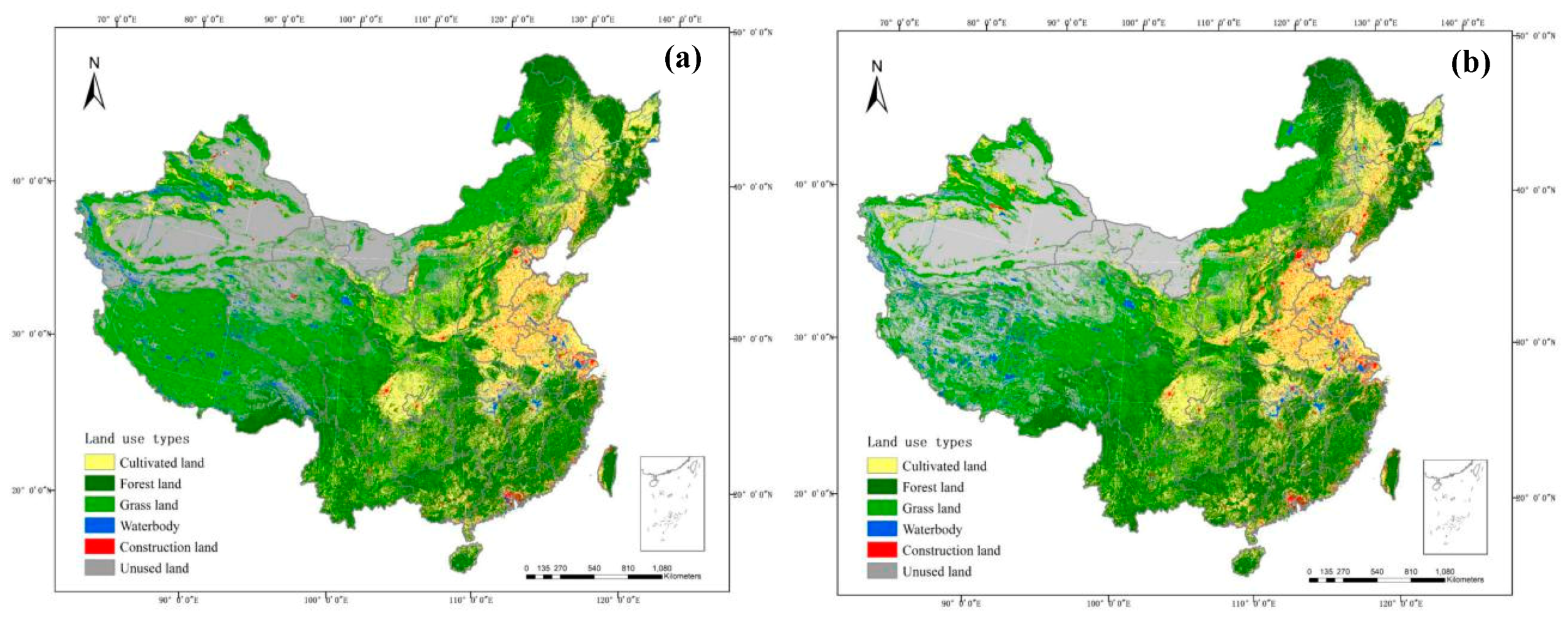
The land use dataset with a spatial resolution of 1 km for the mainland China for the period of 1990 to 2015 was downloaded from the Data Center of the Institute of Geographic Sciences and Natural Resources Research, Chinese Academy of Sciences (http://www.resdc.cn/). Six land use types are included: cultivated land, forest land, grassland, waterbody, construction land and unused land.

The national GDP values at the prefectural level from 1990 to 2015 were obtained from provincial and prefectural statistical yearbooks. Some of the regional data were missing due to the change in administrative boundaries at the prefectural level and the missing data were set to Nodata. Meanwhile, Taiwan, Hong Kong and Macao were not considered in this study.

The outputs of major crops used as coefficients in ESV evaluation were obtained from the China statistical yearbook of 2016 [1]. The major crops in China include rice, wheat, corn and soybeans. The average purchase prices of major crops were provided by the China agricultural product price survey yearbook of 2016 [32]. A summary of all the datasets used in this study is presented in

Table 1. Description of the datasets used in this study.

Data	Time	Scale/Form/Resolution	Source
Land use	From 1990 to 2015	National, 1 km resolution	Institute of Geographic Sciences and Natural Resources Research Chinese Academy of Sciences (http://www.resdc.cn/)
GDP	From 1990 to 2015	National, spreadsheet	National, provincial and prefectural Statistical Yearbook
Outputs of major crops	2015	National, spreadsheet	National Statistical Yearbook
Crops purchase price	2015	National, spreadsheet	National Statistical Yearbook
Administrative Boundaries	2007	National, vector shapefile	Institute of Geographic Sciences and Natural Resources Research Chinese Academy of Sciences (http://www.resdc.cn/)

.

3. Methods

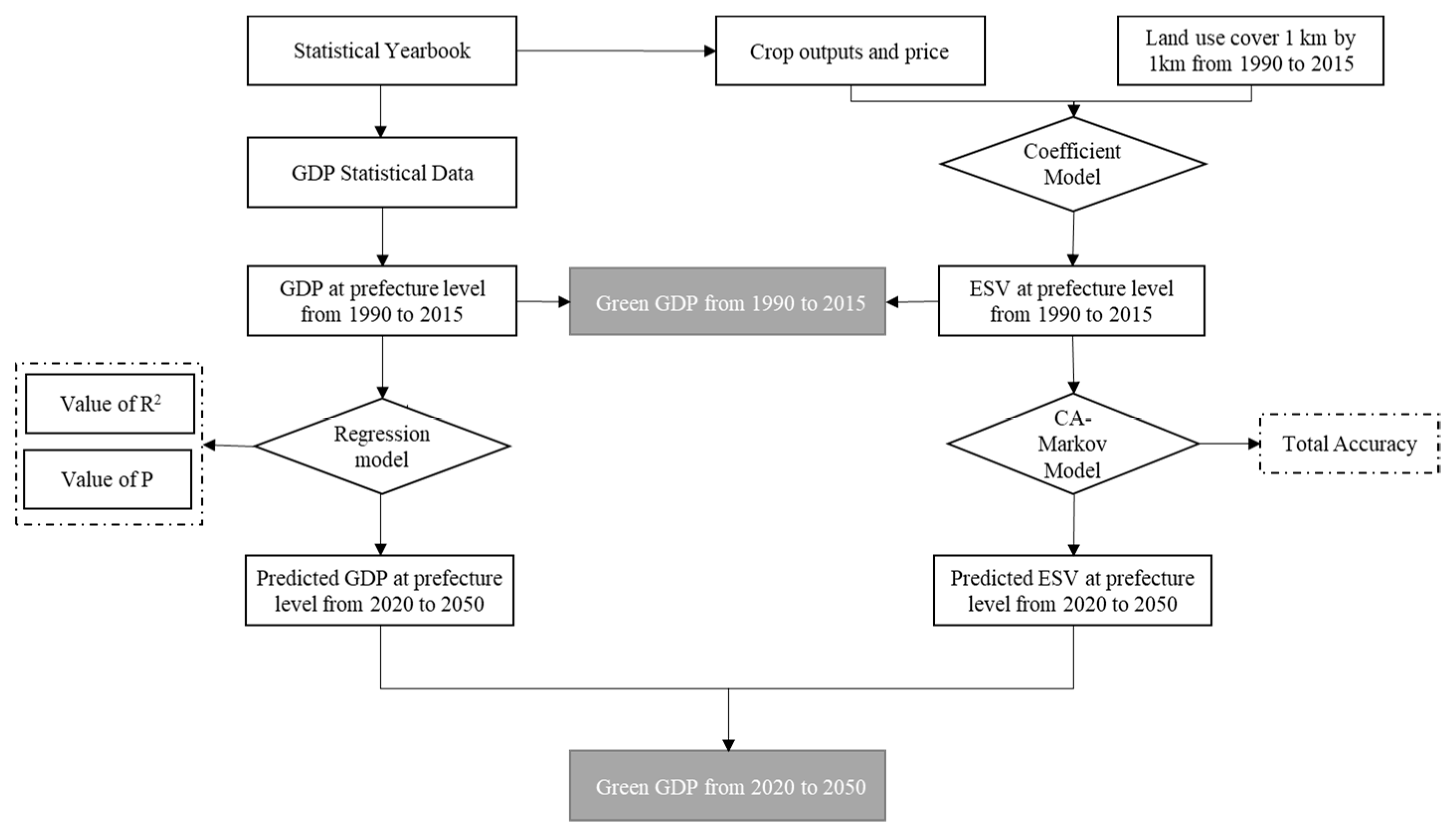
We first used the coefficient method proposed by Costanza et al. [33] to evaluate the ESV in response to land use changes for China from 1990 to 2015 and meanwhile, the GDP at the prefectural level was obtained from provincial and prefectural statistic yearbooks. After accounting for the green GDP for China, we used the CA-Markov model to simulate the land use changes from 2015 to 2050 and the increasing trend of GDP was built by linear regression. The framework of this study is presented in Figure 1.

3.1. Estimation of the Ecosystem Service Value

This study referred to the coefficient method proposed by Costanza et al. [33] to calculate the ESV at the prefectural level for the entirety of China (see Equation (1)):

$$ESV={\displaystyle \sum }_{i=1}^n{A}_i\times E_i,$$

(1)

where $ESV$ is the total value of the regional ecosystem service value; $A_i$ is the area of the i-th land-use; $E_i$ is the ESV coefficient for the i-th land use, which indicate the ESV per unit area of the i-th land-use type (yuan/hm²); and n is the number of land use types. $E_i$ is vital in ESV calculations and can be determined by Equation (2).

$$E_i=e_i\times E_a$$

(2)

$e_i$ is the equivalent factor of the unit price of the ESV of the i-th land-use type (see

Table 2. Equivalent factor of the unit price of the ecosystem service value (ESV) for land use types in 2015 (Units: yuan/hm²).

Land Use Types	${\mathit{e}}_{\mathit{i}}$
Cultivated land	16,538.88 × 108
Forest land	108,095.26 × 108
Grass land	86,873.69 × 108
Waterbody	54,264.14 × 108
Unused land	7357.97 × 108

), which can be determined according to the estimation method of the ecosystem service function value coefficient proposed by Constanza et al. [33] and Xie et al. [34]. $E_a$ represents the economic value of the food production function for per unit area of farmland and can be determined using Equation (3).

$$E_a=\frac{1}{7}{\displaystyle \sum }_{j=1}^k\frac{m_j{p}_j{q}_j}{M}, \left(i=1,\cdots ,k\right)$$

(3)

$j$ is the j-th type of crop and k is the number of crop types. $P_j$ is the national average price of crops in the j-th crop (yuan/ton) and $q_j$ is the yield of the j-th crop (ton/hm²). $m_j$ is the planting area of the j-th crop (hm²). $M$ is the total crop area of all crops (hm²) and 1/7 refers to one-seventh of the economic value of the function of farmland providing food production unit area. According to the status of the main crops in China, wheat, corn, rice and cotton were selected as the major crops. In addition, the $P_j$ can be achieved from a China Yearbook of Agricultural Price Survey [31] for each major crop, and, on the other hand, $q_j$ and $m_j$ can be achieved from the provincial statistical yearbook of 2016. The ESVs from 1990 to 2015 were calculated based on the $E_a$ evaluated by Equation (3) and were expressed in national average prices of crops for 2015 and can reflect the variation in ecosystem service caused by land use change directly.

Since the ESV is a total index for the whole city, we defined the UESV as the ESV in a unit area for a specific city (see Equation (4)).

$${\mathrm{UESV}}_m=\frac{ES{V}_m}{Are{a}_m}$$

(4)

${\mathrm{UESV}}_m$ is the value of the ecological services of the m-th city on its per unit area (yuan/hm²) and $Are{a}_m$ is the area of the m-th city (hm²).

3.2. Estimation of Green GDP

Green GDP was proposed to reflect the development of economy and ecological preservation simultaneously and it can be measured as Equation (5) shows.

$$G_m=TES{V}_m+GD{P}_m$$

(5)

$G_m$ refers to the value of green GDP for the m-th city. $TES{V}_m$ is the ecological service value for the m-th city. $GD{P}_m$ is the gross domestic product for the m-th city.

3.3. ESV Forecasting Based on the CA-Markov Model

Because ESV is measured according to land use pattern, we simulated the future land use pattern by the CA-Markov model first and then forecasted the ESV in the future. CA can be expressed by Equation (6).

$${\delta }_i+1=f\left(St,N\right)$$

(6)

$\delta$ is a finite and discrete set of states of the cell. $N$ is the neighborhood of the cell, $t$ and $t+1$ refer to a different time of iteration. $f$ is the transformation rule of the state of the local space cell [35].

The Markov method uses Markov chain theory and probability theory to analyze the law of random event changes. This method was used to predict a long-term prediction method in the future state of change in each period [36].

$$S_{\left(t+1\right)}=P_{ij}\times S_{\left(t\right)}$$

(7)

$S\left(t+1\right)$ is the state of the land use system at time $t+1$. $P_{ij}$ is the state of the land use system at time $t$. $S\left(t\right)$ is the transfer matrix.

Both the CA model and the Markov model are dynamic models with discrete states. The CA-Markov model combines the advantages of the CA model to simulate spatial variations of complex systems and the advantages of the Markov model for quantitative prediction [27,37]. With the combined advantages of CA and Markov, the CA-Markov model has been widely used in land use space simulation applications [38].

To reflect the regional characteristics and regional differences in land use changes, according to the existing research [39,40,41], the entire country was divided into four regions—eastern, central, western and northeast—in the process of future land use simulation based on the 16th National Congress of the Communist Party of China. After the land use simulation for each region separately, we used the merging tool in ArcGIS to combine the results so as to obtain the final land use pattern for the entirety of China. Detailed descriptions of the four regions are listed in

Table 3. The descriptions of the four sections in the CA-Markov land use simulation.

Region Index	Name	Zone	Abbreviation
Z1	Eastern China	Beijing, Tianjin, Hebei, Shandong, Jiangsu, Shanghai, Zhejiang, Fujian, Guangdong, Hainan, Taiwan, Macao and Hong Kong	EC
Z2	Northeast China	Heilongjiang, Jilin and Liaoning	NEC
Z3	Western China	Inner Mongolia, Ningxia, Shaanxi, Chongqing, Guizhou, Guangxi, Yunnan, Sichuan, Gansu, Qinghai, Xinjiang and Tibet	WC
Z4	Central China	Shanxi, Henan, Anhui, Hubei, Hunan and Jiangxi	CC

. To carry out the simulation, the CA-Markov module in IDRISI software was used.

3.4. Gross Domestic Product Forecasting Based on the Regress Model

According to the statistical yearbook from 1990 to 2016, the GDP at the prefectural level was obtained. A linear regression model was built up to predict the GDP for 2020-2050. Specifically, years were considered as the independent variable and GDP at the prefectural level was set as the dependent variable in the regression, as Equation (8) shows:

$$Y=\propto x+\beta ,$$

(8)

where $Y$ is the dependent variable of GDP; $\propto$ and $\beta$ are the regression coefficients; and $x$ is the independent variable of years.

We also defined the UGDP to indicate the GDP value on per unit area in a specific city (see Equation (9)):

$$UGD{P}_m=\frac{GD{P}_m}{Are{a}_m},$$

(9)

where $UGD{P}_m$ is the GDP value for per unit area of the m-th city (thousand yuan/hm²) and $Are{a}_m$ is the area of the m-th land use (hm²).

4. Results

4.1. Temporal and Spatial Variations of ESV from 1990 to 2015

According to the national 11th Five-Year Plan, the whole nation can be classified into four major sections: the eastern region, central region, western region and northeastern region. To display and analyze the differences in ESV, GDP and green GDP in the regions in detail, we divided the four major regions into eight major economic zones by referring to existing studies [42,43]. Descriptions of the eight major economic zones are listed in

Table 4. Descriptions of China’s eight economic zones and abbreviations.

Region Index	Name	Zone	Abbreviation
A	Northeast Economic Zone	Liaoning, Jilin, Heilongjiang	NEEZ
B	Northwest Economic Zone	Gansu, Qinghai, Ningxia, Tibet and Xinjiang	NWEZ
C	Middle Reaches of the Yellow River Economic Zone	Shaanxi, Shanxi, Henan and Inner Mongolia	MYREZ
D	Northern Coastal Economic Zone	Beijing, Tianjin, Hebei and Shandong	NCEZ
E	Eastern Coastal Economic Zone	Shanghai, Jiangsu and Zhejiang	ECEZ
F	Middle Yangtze River Economic Zone	Hubei, Hunan, Jiangxi and Anhui	MYTREZ
G	Southwest Economic Zone	Yunnan, Guizhou, Sichuan, Chongqing and Guangxi	SWEZ
H	Southern Coastal Economic Zone	Fujian, Guangdong and Hainan	SCEZ

. The differences, variations and trends for ESV, GDP and green GDP were analyzed at the economic zone level.

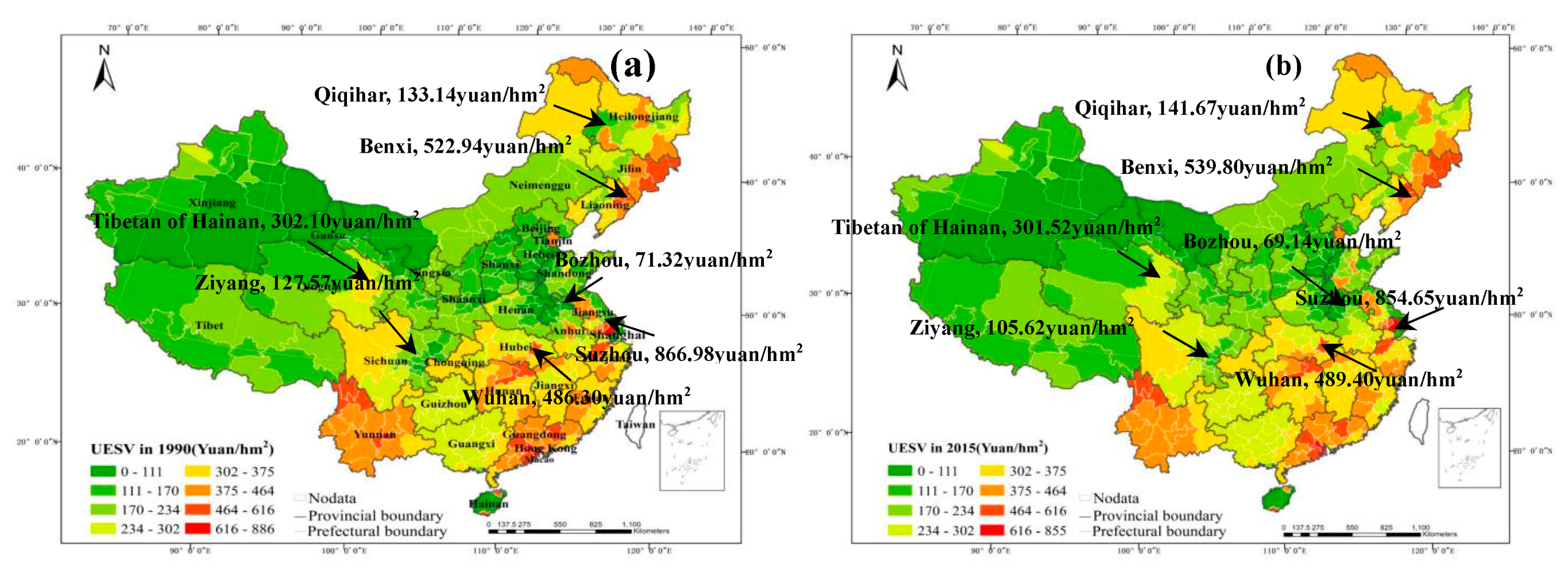
As the results showed, UESV gradually increased from northwest to southeast (see Figure 2). This pattern was consistent with the spatial distribution of major forests in China. The better the hydrothermal conditions, the higher the value of ecosystem services would be. The UESV has been analyzed for 2015 (see

Table 5. The maximum and minimum values of UESV in 2015 (Units: yuan/hm²).

	The Maximum Value of UESV	The City with the Maximum Value of UESV	The Minimum Value of UESV	The City with the Minimum Value of UESV	The UESV Value
NEEZ	539.80	Benxi	141.67	Qiqihar	325.14
NWEZ	301.52	Tibetan Autonomous Prefecture of Hainan	44.92	Jiuquan	140.13
MYREZ	347.42	Hulun Buir	51.85	Alxa League	195.25
NCEZ	429.70	Tianjin	65.46	Langfang	179.57
ECEZ	854.65	Suzhou	137.95	Yancheng	354.41
MYTREZ	609.69	Ezhou	69.14	Bozhou	323.10
SWEZ	506.71	Nujiang Lisu Nationality Autonomous	105.62	Ziyang	320.29
SCEZ	831.49	Foshan	246.22	Xiamen	420.35

). The economic zones with high values of UESV mainly included the SCEZ, with a UESV value of 420.35 yuan/hm² and the ECEZ, with a UESV value of 354.41 yuan/hm². The high values of UESV in the SCEZ and ECEZ are probably due to better hydrothermal conditions and higher vegetation coverage, such as for Foshan city in Guangdong province, with a UESV of 831.49 yuan/hm² and Suzhou city in Jiangsu province, with a UESV value of 854.65 yuan/hm², whereas the lowest values of UESV, 246.22 yuan/hm² and 137.95 yuan/hm², were for Xiamen city and Yancheng city, respectively. The NEEZ, MYTREZ and SWEZ experienced the second highest UESV. To be specific, the UESV values in the NEEZ, MYTREZ and SWEZ were 325.14 yuan/hm², 323.10 yuan/hm² and 320.29 yuan/hm², respectively. In particular, in the SWEZ, the high value of UESV, 506.71 yuan/hm², was concentrated in Nujiang city in Yunnan province. Usually, in the SWEZ, the places with rich hydrothermal conditions in Yunnan province tended to maintain high values of UESV. On the other hand, Ziyang city in Sichuan suffered the lowest USEV value of 105.62 yuan/hm² in the SWEZ.

Typically, in the NEEZ, the high values of UESV are probably due to the fact that there are massive forest reserves in the NEEZ and forests are an important carbon pool in China [44]. Some places in the NEEZ trended to maintain the highest average UESV of 539.80 yuan/hm², such as Benxi city in Liaoning province. However, some places in the NEEZ also experienced lower UESV, such as Qiqihar city in Heilongjiang province, with a UESV value of merely 141.67 yuan/hm². In the MYTREZ, the high values of UESV were distributed in the highly developed central cities, such as Wuhan city in Hubei province and Changsha city in Hunan province, which have well-developed waterbodies and relatively rich forest lands, with UESVs of up to 489.40 yuan/hm² and 360.67 yuan/hm², respectively. On the other hand, the lowest UESV was located in Bozhou city in Anhui province for the MYTREZ, which had few forest lands, with a UESV of only 69.14 yuan/hm². As for the SWEZ, the places with rich hydrothermal conditions in Yunnan tended to maintain high values of UESV. On the other hand, Ziyang city suffered the lowest USEV value of 105.62 yuan/hm² in the SWEZ.

The NWEZ, MYREZ and NCEZ suffered the lowest UESV. The shortage of waterbodies and massive unused land covers resulted in relatively low UESV values in the NWEZ, MYREZ and NCEZ, which were 140.13 yuan/hm², 195.25 yuan/hm² and 179.57 yuan/hm², respectively. The maximum UESV values in the NWEZ, MYREZ and NCEZ were merely 301.52 yuan/hm², 347.42 yuan/hm² and 429.70 yuan/hm² in the Tibetan Autonomous Prefecture of Hainan, Hulun Buir city and Tianjin, respectively.

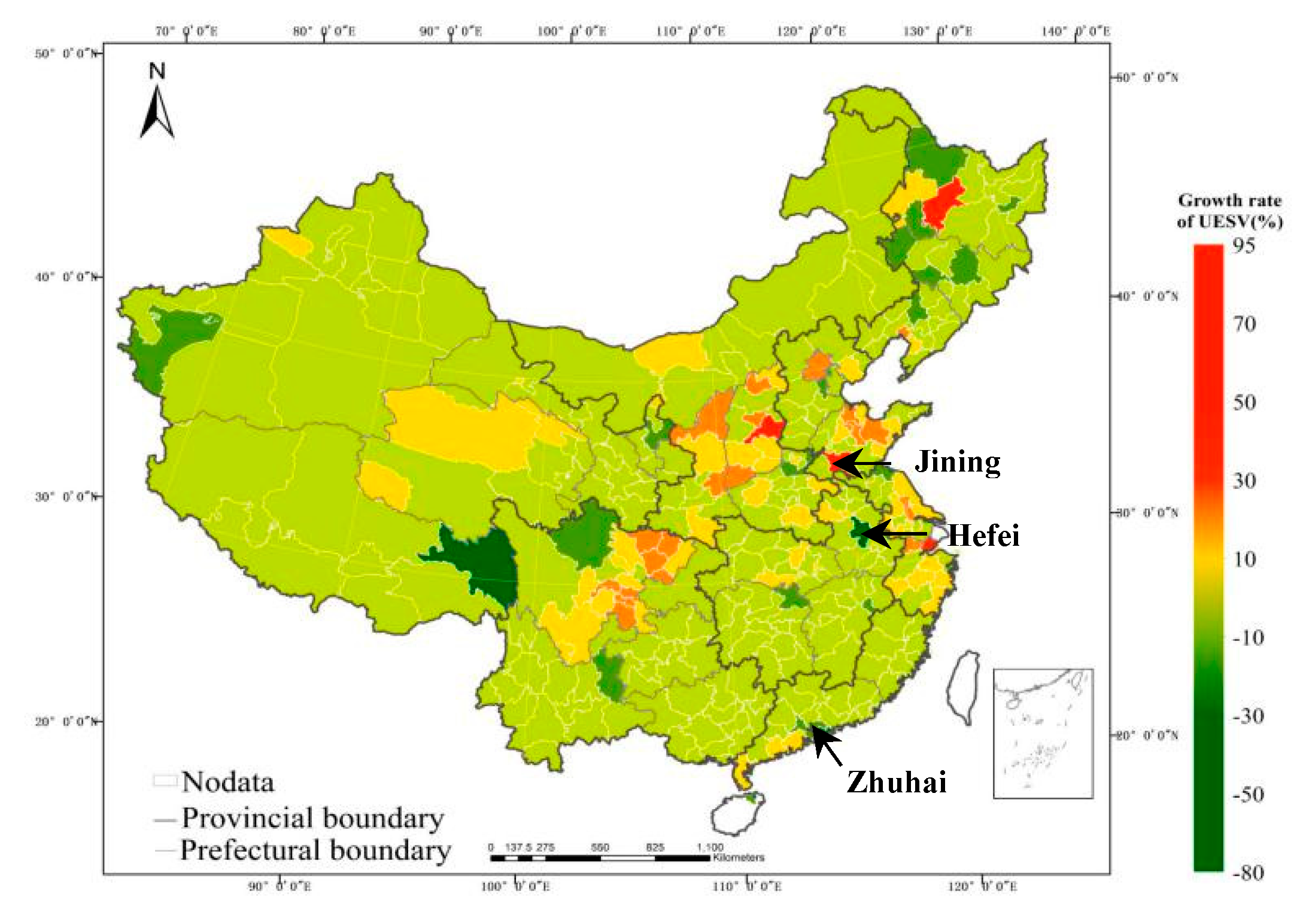
The total ESV for China experienced an obvious decreasing trend from 1990 to 2015, with the average UESV dropping 1004.64 yuan/hm². Most of China has suffered from an approximately 10% decline in ESV (see the green area in Figure 2). Specifically, the UESV in the NWEZ, MYTREZ and SWEZ showed an obvious decreasing trend, with decreases of 1.72 yuan/hm², 108.62 yuan/hm² and 6.35 yuan/hm² from 1990 to 2015, respectively. Among them, the forest land and grassland decreased and the construction land increased over large areas of Hefei city, which suffered the greatest decrease from 427.08 yuan/hm² in 1990 to 248.31 yuan/hm² in 2015. However, UESV in some areas still showed slight growth. For example, the UESV in the ECEC, MYREZ, NCEZ and SCEZ grew by 22.90 yuan/hm², 49.83 yuan/hm², 54.72 yuan/hm² and 5.23 yuan/hm² from 1990 to 2015, respectively. Waterbodies enlarged Jining city in Shandong province and Zhuhai city in Guangdong province, which maintained large increases of 178.35 yuan/hm² and 164.31 yuan/hm², respectively (see Figure 3).

4.2. ESV Forecasting Based on Future Land Use Change

4.2.1. Future Land Use Simulation

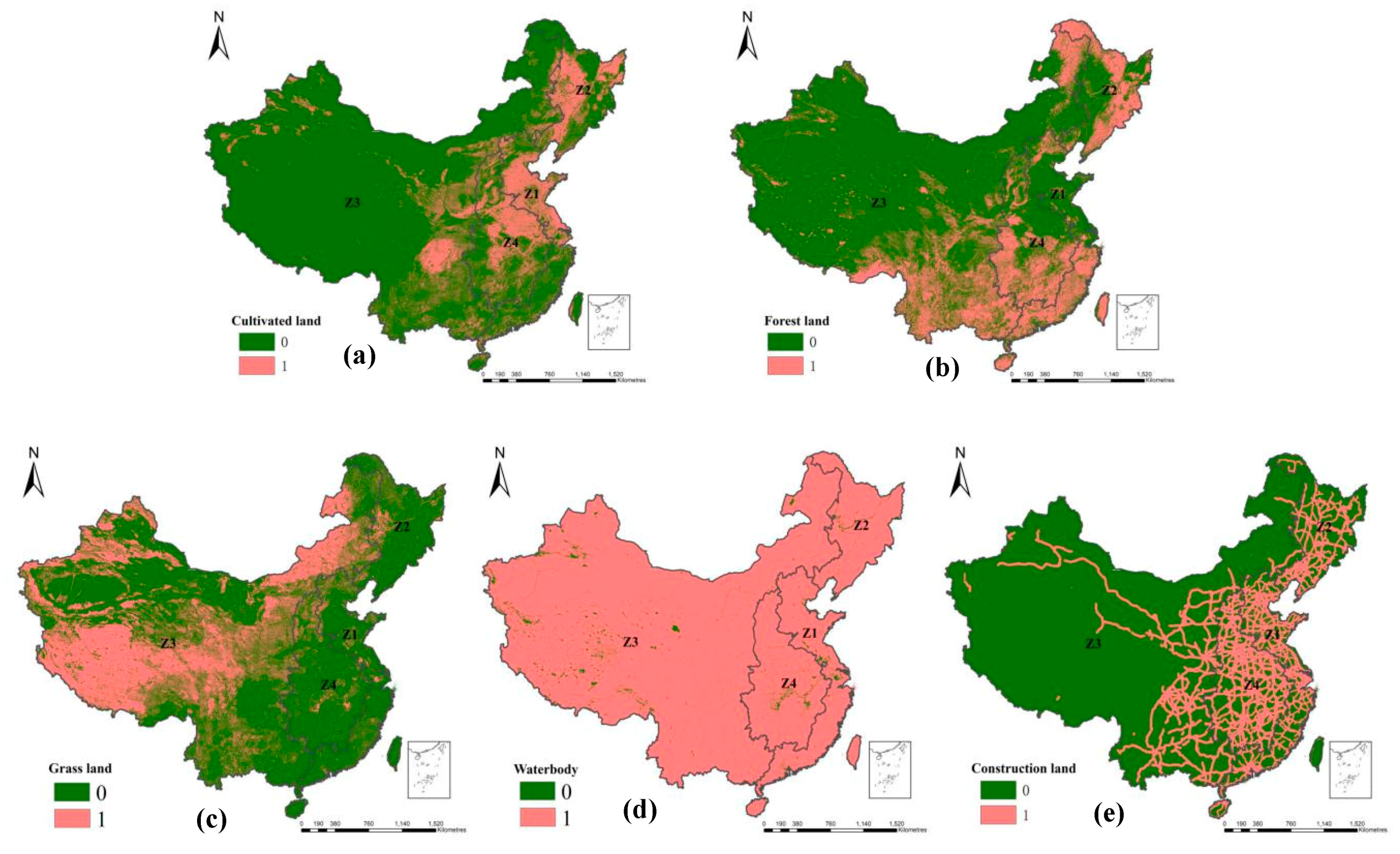
To reduce the uncertainty in the land use simulation, this study used the CA-Markov model to determine land suitability so as to guide the land use simulation process. The land use characteristics and geographical conditions were different in the four regions. For example, in the northeast, eastern and central regions, cultivated land was the main land use type and the transportation network was dense without steep slopes in regions. However, in the western region, most areas were covered by unused land with a low density of built-up land and transportation networks. Therefore, according to the different natural characteristics of each region, the suitability atlas calculation process differed for different regions, which was set as follows.

(1) Selection of impact factors:

There were many constraints for different land uses. Various impact factors such as the slope, distance to transportation networks and distance to the waterbody can be used to determine the constraints for land uses.

(2) Establishment of suitability maps for land uses

Cultivated land: First, the places covered with cultivated land were set to 1. Otherwise, they would be set to 0. Moreover, the places covered with unused land in Z1, Z2 and Z4 were set to 1, indicating that the unused land in those regions can be transformed into cultivated land. However, the unused land in Z3 was set to 0, since the unused land in Z3 is usually desert, frozen ground or other land uses and cannot be developed. Therefore, the places covered with unused land in Z3 were set to 0. According to the national Regulations on the Work of Water and Soil Conservation [45], cultivated land cannot be located in places with slopes larger than 25 degrees. Therefore, the suitability for cultivated land was set to 0 at places with slopes exceeding 25 degrees.

Forest land: According to the transfer matrix, the grass land can be transferred to forest land. Therefore, the places with grass land were set to 1. Meanwhile, it was then determined that the forest land tended to be located in places close to waterbodies. It is learned that in Z1, 73% of the forest land was located in places within 550 km of a waterbody. Therefore, we selected a threshold of 550 km as a constraint, indicating that a place is suitable for forest land. Otherwise, the places would be set to 0. As for Z2, Z3 and Z4, similarly, the distance thresholds for waterbodies have been set to 450 km, 880 km and 420 km when 71%, 77% and 72% forest land, respectively, is located within those distances from waterbodies. Similar to cultivated land, for forest land, the places with unused land in Z1, Z2 and Z4 were set to 1, indicating that those places are capable of being converted to forest land.

Grass land: According to the land use transfer matrix, forest land can be converted to grass land. Therefore, the places covered by forest land and grass land were set to 1 first. Meanwhile, it is also found out that the grass land tended to be located close to waterbodies. We set the threshold distance such that 70% grassland was located in the distance buffer. Specifically, the threshold distances from a waterbody for Z1, Z2, Z3 and Z4 were 550 km, 420 km, 850 km and 400 km, respectively. Last, the places covered by unused land in Z1, Z2 and Z4 were set to 1.

Waterbody: Transfers and development were not allowed for waterbodies. Therefore, the places with waterbody types were set to 1 and the other places were set to 0.

Construction land: First, the places with construction land were set to 1. It was then determined that the construction land tended to be located in the places close to transportation networks. Therefore, we selected the threshold distances from transportation networks when there was 75% construction land located in those buffer areas. Specifically, the threshold distances were 800 km, 900 km, 1350 km and 1000 km for Z1, Z2, Z3 and Z4, respectively.

The suitability maps for different land uses were obtained at the national scale and are presented in Figure 4.

The land uses in 2015 were simulated based on land use in 2010 and land use changes from 2005 to 2010 were used to verify the model (see

Table 6. Transition probability matrix of land use change from 2005 to 2010.

Land Use Type		2010
		Cultivated Land	Forest Land	Grass Land	Waterbody	Construction Land	Unused Land
2005	Cultivated land	0.9939	0.001	0.0007	0.0006	0.004	0.0001
	Forest land	0.0007	0.9983	0.0006	0.0012	0.0005	0.0001
	Grass land	0.0023	0.0007	0.9942	0.0015	0.0002	0.0008
	Waterbody	0.0015	0.0002	0.0014	0.9946	0.0016	0.0017
	Construction land	0.0006	0.0004	0.0034	0.0009	0.9942	0.0003
	Unused land	0.0012	0	0.001	0.0013	0.0002	0.9976

). The Markov model was used to calculate the land use transfer matrix and then quantitatively explained the transformation among land-use types from 2005 to 2010. Then, based on the suitability maps and transfer matrix, the land use spatial pattern was simulated for 2015 (see Figure 5). The simulation results indicated that the simulation accuracies in Z1, Z2, Z3 and Z4 were 84%, 81%, 91% and 88%, respectively. According to existing studies, the accuracies of our model were acceptable [46,47]. Therefore, the model can be used for further forecasting of the spatial distribution.

The verified model with land use transfer matrix from 2005 to 2010 was then used to simulate the future land use patterns for Z1, Z2, Z3 and Z4. The results indicated that the areas of cultivated land, grassland and unused land in the next 30 years will dynamically decrease with decline rates of −8.71%, −2.97% and −9.28%, respectively (see

Table 7. Land use change from 1990 to 2050 (Units: 10⁶ hm²).

			Forecast Data from 2020 to 2050
Year	1990	2015	2020	2025	2030	2035	2040	2045	2050	Growth Rate (%)
Cultivated land	177.18	178.6	181.25	178.43	175.35	172.29	169.4	165.65	161.75	−8.71
Forest land	225.5	224.02	228.99	230.7	232.04	237.24	240.44	244.58	252.1	11.80
Grass land	300.19	295.4	264.93	268.33	267.27	258.39	262.57	276.81	291.28	−2.97
Waterbody	27.05	28.01	26.9	27.41	27.74	27.17	27.08	26.98	28.13	3.99
Construction land	15.86	22.19	25.01	25.46	26.54	27.46	28.63	29.93	31.17	96.53
Unused land	200.89	198.45	219.59	216.34	217.73	224.12	218.55	202.72	182.24	−9.28

). By contrast, forest land, waterbody and construction land will increase by 11.80%, 3.99% and 96.53%, respectively (see Table 7). Some regions in particular experienced sharp growth in construction land, such as Z1 and Z3, with increases of 6.75×10⁶ hm² and 15.48×10⁶ hm², respectively. On the other hand, the areas of cultivated land, grass land and unused land were largely decreased in the western region, those losses being 15.42×10⁶ hm², 12.50×10⁶ hm² and 15.24×10⁶ hm², respectively (see

Table 8. Land use growth changes in Z1, Z2, Z3 and Z4 from 1990 to 2050 (Units: 10⁶ hm²).

	Cultivated Land	Forest Land	Grass Land	Waterbody	Construction Land	Unused Land
Z1	−6.52	2.81	−3.02	0.01	6.75	−0.03
Z2	0.18	2.36	−2.82	−0.15	3.28	−2.85
Z3	−15.42	26.61	−12.50	1.07	15.48	−15.24
Z4	−11.78	7.80	−3.66	−0.06	9.31	−1.61

).

4.2.2. Forecasted ESV from 2020 to 2050

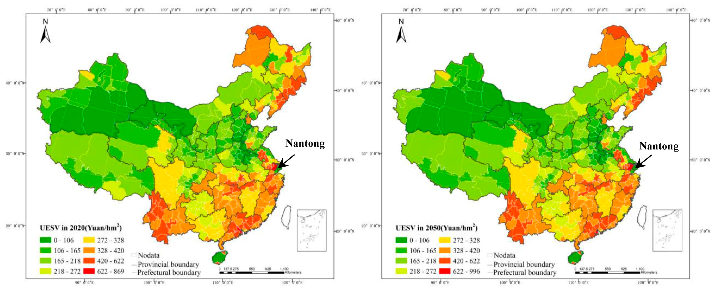
Based on the simulated future land use pattern, the ESV from 2020 to 2050 was measured. In terms of spatial variation, it was found that the high values of UESV were mainly distributed in coastal and northeast China, such as the SCEZ and ECEZ (see Figure 6). Specifically, the UESV in the SCEZ would be up to 421.35 yuan/hm² in 2050, with the UESV in the ECEZ following at 361.85 yuan/hm² in 2050. According to our results, the overall pattern of UESV was ranked as the SCEZ > ECEZ > MYTREZ > NEEZ > SWEZ > MYREZ > NCEZ > NWEZ in 2050.

In terms of temporal variation, the UESV was gradually decreased from 2020 to 2050, with a total reduction of 1108 yuan/hm² and rate of growth of −1.21% (

Table 9. The variations in UESV in regions from 2020 to 2050 (Units: Yuan/hm²).

Economic Zone	2020	2025	2030	2035	2040	2045	2050	Growth Rate (%)
NEEZ	319.80	324.64	324.26	320.70	324.79	322.71	320.63	0.259
NWEZ	144.48	144.04	147.06	144.06	144.06	144.59	144.09	−0.270
MYREZ	196.89	197.31	197.32	209.28	197.32	197.37	197.26	0.188
NCEZ	173.76	170.63	171.78	170.42	170.59	170.19	170.34	−1.967
ECEZ	367.40	361.78	361.90	361.97	362.23	362.06	361.85	−1.511
MYTREZ	324.57	325.18	325.19	325.14	317.93	323.50	325.05	0.148
SWEZ	324.31	333.80	324.39	321.37	324.37	324.28	290.16	−10.530
SCEZ	421.33	421.41	421.59	411.44	421.46	421.53	421.35	0.004

). The ESV in the SWEZ, NCEZ and ECEZ showed a decreasing trend, with reducing rates of −10.53%, −1.968% and −1.512%, respectively. As an example, the maximum decline rate of Nantong city was −43.91% (see Figure 6). The UESV in the NWEZ showed a slight downward trend, with reductions of −0.268%.

A slight upward trend of UESV was detected in the NEEZ, MYREZ, MYTREZ and SCEZ with increases of 0.259%, 0.188%, 0.148% and 0.004%, respectively. For the SCEZ and NEEZ, it is probably because of increasing forest land in these two regions. Specifically, in the SCEZ and NEEZ, the forest land increases by 1.38×10⁶ hm² and 3.21×10⁶ hm², respectively. A larger area of forest land (with $e_i$ of 108,095.26×10⁸ yuan/hm²) would lead to a higher value of ecological service. On the other hand, even if the construction land increases by 1.30×10⁶ hm² and 1.78×10⁶ hm² in both regions, it trended to cover the other land uses with lower ecological service values, such as unused land (with $e_i$ of 7357.97×10⁸ yuan/hm²) and cultivated land (with $e_i$ of 0 yuan/hm²). Therefore, an increasing trend has been detected in these regions.

4.3. Temporal and Spatial Variations of GDP from 1990 to 2015

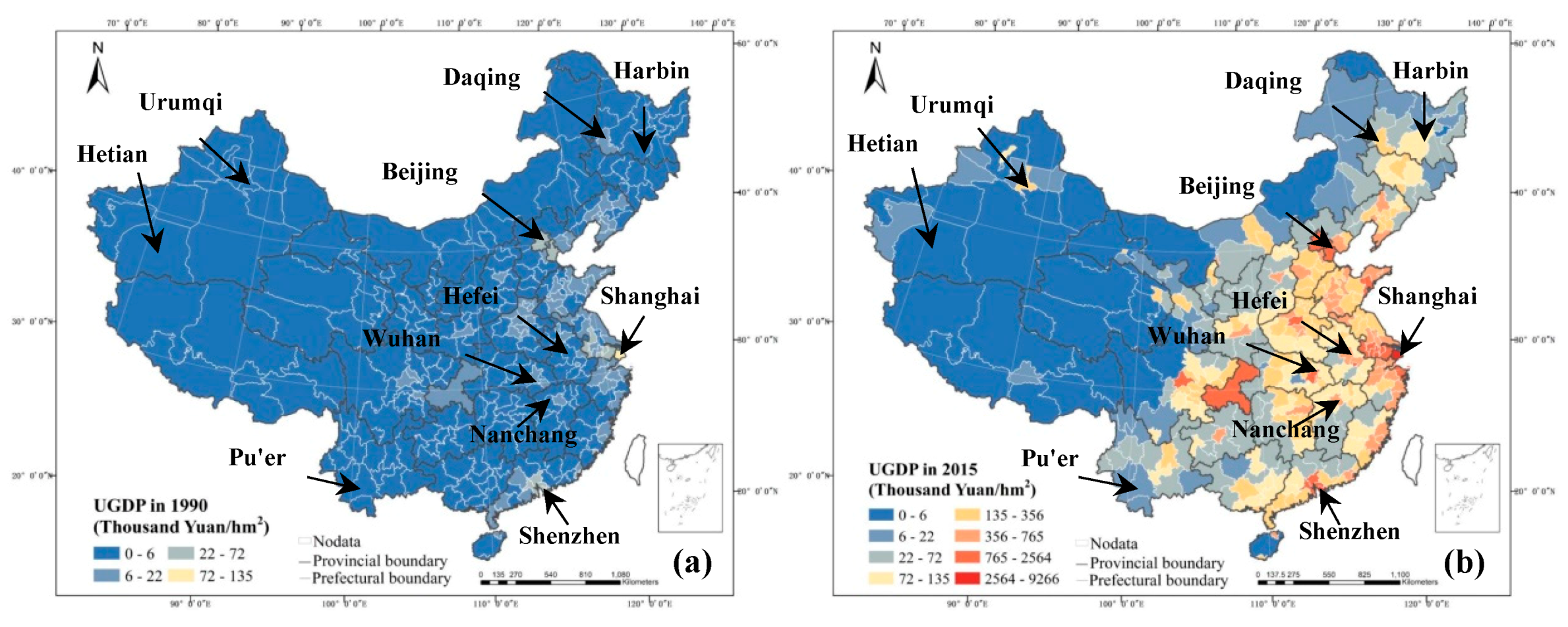
The results indicated that in 2015, the UGDP decreased from the southeast to the northwest and the high values of UGDP were mainly concentrated in the NEEZ, ECEZ and SWEZ (see Figure 7). In addition, it was also found that the UGDP trended to be much higher in one or two cities than the UGDPs of the surrounding cities. For example, the average UGDPs in Shenzhen city (3051.39 thousand yuan/hm²) and Guangzhou city (877.10 thousand yuan/hm²) were the highest in Guangdong province, whereas the average UGDP for other cities in Guangdong province was merely 211.18 thousand yuan/hm² in the period from 1990 to 2015.

The spatial differences in UGDP in China became more severe from 1990 to 2015. For example, the maximum UGDP of Shenzhen city was up to 72.00 thousand yuan/hm² in Guangdong province and the maximum UGDP of Urumqi city in Xinjiang province was merely 4.00 thousand yuan/hm² in 1990; that gap was up to 9077.00 thousand yuan/hm² in 2015. Different growth rates in different regions led to this spatial difference in UGDP in 2015.

The UGDP showed an obvious upward trend in the ECEZ, SCEZ and NCEZ. For example, Shenzhen city, Shanghai city and Beijing city experienced the largest growth, with increases of 9193.81 thousand yuan/hm², 4329.82 thousand yuan/hm² and 1369.45 thousand yuan/hm² from 1990 to 2015, respectively.

The growth rates of the NEEZ and MYTRZE were moderate. Traditional industrial cities in the NEEZ experienced higher development than other cities in NEEZ. For example, the UGDPs in Harbin city and Daqing city were increased by 106.23 thousand yuan/hm² and 133.78 thousand yuan/hm², with growth rates of 98.05% and 94.97%, respectively. Capital cities, for example, Wuhan in Hubei province, Hefei in Anhui province and Nanchang city in Jiangxi province in the MYTREZ, experienced greater growth than did other cities in the MYTREZ and accounted for 41.13%, 13.20%, 30.79% and 29.8% of the total UGDP for the whole region of the MYTREZ in 2015.

However, the NWEZ, SWEZ and MYREZ experienced relatively low growth rates. For example, the UGDP of Hetian in Xinjiang province, Pu’er in Yunnan province and Yushu in Qinghai province experienced the lowest growths of 0.94 thousand yuan/hm², 0.91 thousand yuan/hm² and 0.73 thousand yuan/hm² from 1990 to 2015, respectively.

4.4. GDP Forecasting from 2020 to 2050

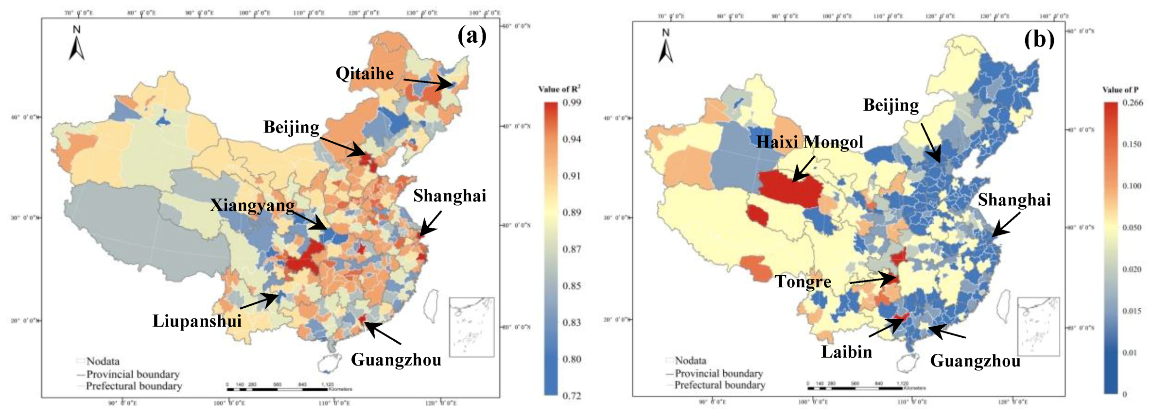
Based on the temporal changes in GDP, a linear regression was built up for each city to predict the GDP in 2020 to 2050. The values of R square and significant P for the regressions of each city are presented in Figure 8a. It is noted that the values of R square for most of the cities were in the range of 0.72 and 0.99, indicating a high fitting accuracy. Specifically, the R square was larger in the highly developed cities of China, such as Beijing (with R square of 0.95), Shanghai (with R square of 0.98) and Guangzhou (with R square of 0.95). However, R square was lower in those eastern cities suffering depressed development, such as Qitaihe in Heilongjiang (with R square of 0.72), Liupanshui in Guizhou province (with R square of 0.75) and Xiangyang in Hubei province (with R square of 0.76). In statistics, a significant P less than 0.05 and greater than 0.01 indicates statistical significance and P less than 0.01 indicates very significant. However, the significant P exceeded 0.05, indicating that the difference was not significant. The significant P was closer to 0.01 in most of the highly developed cities (see Figure 8b), such as Beijing (with P of 0.007), Shanghai (with P of 0.003) and Guangzhou (with P of 0.007). However, values of P exceeded 0.05 in the economically under-developed areas, for example, Haixi Mongol (with P of 0.266) in Qinghai province, Laibin (with P of 0.154) in the Guangxi Zhuang Autonomous Region and Tongren (with P of 0.157) in Guizhou province. According to the regression model, the GDP value for each city from 2020 to 2050 was predicted.

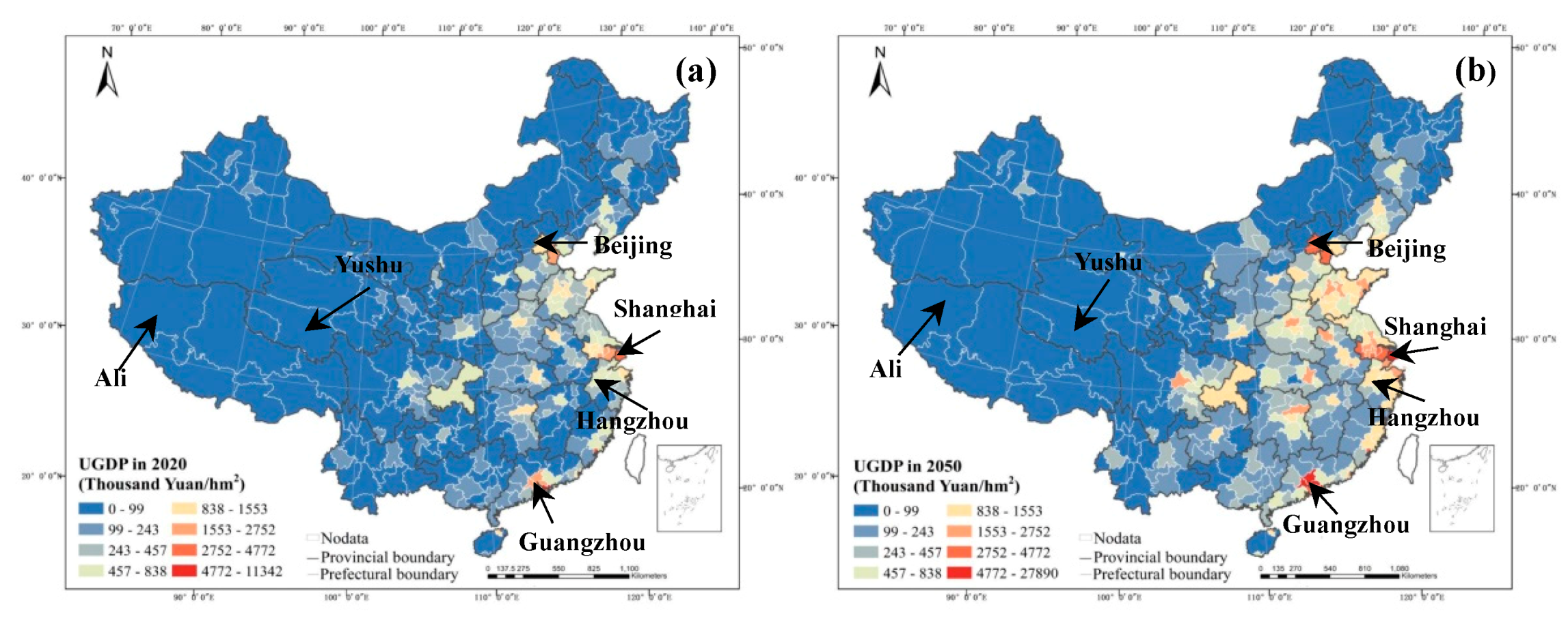
The predicted GDP was presented as the UGDP value for each city in 2020 and 2050 (see Figure 9). According to the results, a huge increase in GDP has been detected—the total national GDP increases from 85,271.13 billion yuan in 2020 to 180,718.28 billion yuan in 2050. The increase is mainly concentrated in the highly developed cities, such as Beijing city, Shanghai city, Guangzhou city and Hangzhou city and the sum of GDP values is as large as 21,847.24 billion yuan, contributing 23.76% of the entire national GDP value in 2050.

As a result, the spatial differences in UGDP become stronger from 2020 to 2050. The high value regions of UGDP were mainly distributed in the ECEZ and SCEZ, with values of 45,061.62 thousand yuan/hm² and 68,205.96 thousand yuan/hm², respectively, in 2050. High UGDP values in the ECEZ and SCEZ are primarily found in Shanghai city, Hangzhou city and Guangzhou city; for 2050, their values were 9949.94 thousand yuan/hm², 1279.45 thousand yuan/hm² and 5405.24 thousand yuan/hm², respectively. In contrast, the UGDP values in the NWEZ and SWEZ were only 4363.51 thousand yuan/hm² and 16,449.02 thousand yuan/hm², respectively, in 2050. In the NWEZ and SWEZ, the lowest UGDPs were located in the blue area in Figure 9, such as Ali in Tibet province and Yushu in Qinghai province, with values of 0.33 thousand yuan/hm² and 0.97 thousand yuan/hm², respectively, in 2050. In the ECEZ and SCEZ, the difference between the high value of UGDP and the low value of UGDP in the NWEZ and SWEZ was 46,135.58 thousand yuan/hm² in 2020 and then the difference was 93,689.98 thousand yuan/hm² in 2050; therefore, the spatial difference was greater between 2020 and 2050.

4.5. Temporal and Spatial Variations of Green GDP from 1990 to 2050

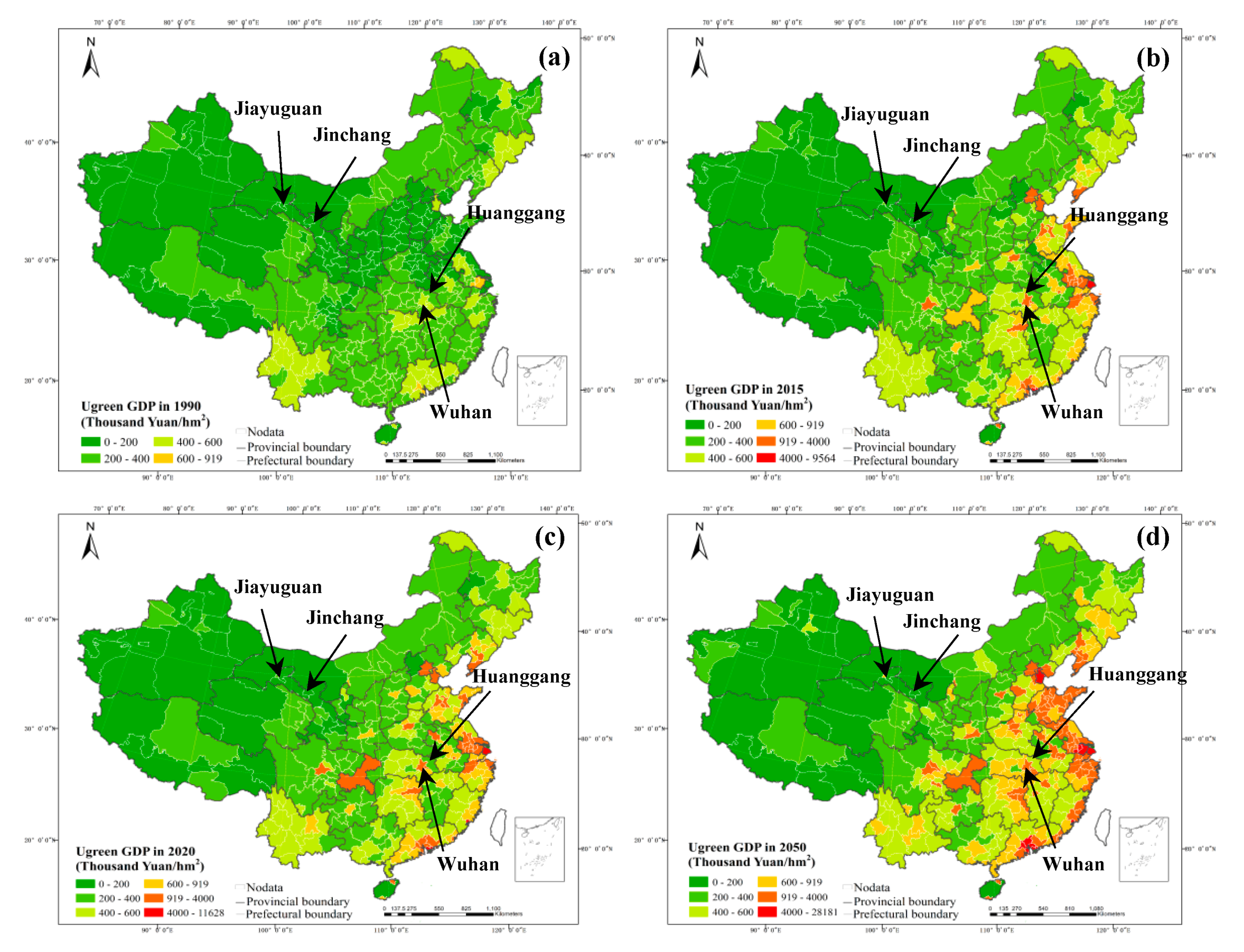
The green GDP was measured according to ESV and GDP at the prefectural level and a huge increase has been revealed from 1990 to 2050. It was found that the green GDP increased from 19,623.94 billion yuan in 1990 to 194,978.29 billion yuan in 2050. Even if the ESV was decreasing, due to the rapid economic development growth, the national green GDP was increasing.

In terms of spatial distribution (see Figure 10), high values of green GDP tended to be located in the south China and east coastal regions, such as Beijing city, Shenzhen city and Guangzhou city, having green GDP of 5006.06 billion yuan, 5273.93 billion yuan and 3910.14 billion yuan in 2050. In addition, low values of green GDP tended to be located in west China, such as Jinchang and Jiayuguan in Gansu province, having green GDP of 75.33 billion yuan and 63.50 billion yuan in 2050. To be specific, the economic zones can be ranked as follows according to their green GDP values in 2050: NCEZ > MYTREZ > SWEZ > MYREZ > ECEZ > SCEZ > NEEZ and NWEZ (

Table 10. Statistics of total ESV, GDP and green GDP in eight districts in 1990 and 2050 (Billion Yuan) and the proportions of ESV and GDP in green GDP (%).

	1990					2050
	ESV	Proportion of ESV in Green GDP	GDP	Proportion of GDP in Green GDP	Value of Green GDP	ESV	Proportion of ESV in Green GDP	GDP	Proportion of GDP in Green GDP	Green GDP
NEEZ	2547.46	93.29	183.10	6.71	2730.56	2489.93	15.66	13,414.89	84.34	15,904.82
NWEZ	3580.29	99.06	33.99	0.94	3614.28	5747.21	47.10	6456.22	52.90	12,203.43
MYREZ	3184.91	97.72	74.33	2.28	3259.24	3268.02	12.66	22,540.06	87.34	25,808.08
NCEZ	599.23	71.15	242.93	28.85	842.16	620.36	1.73	35,244.08	98.27	35,864.44
ECEZ	698.20	71.13	283.33	28.87	981.53	733.46	2.80	25,457.61	97.20	26,191.07
MYTREZ	2264.68	95.78	99.89	4.22	2364.57	2270.84	8.46	24,566.68	91.54	26,837.52
SWEZ	4298.28	97.66	103.05	2.34	4401.33	3920.97	14.71	22,726.93	85.29	26,647.87
SCEZ	1242.60	86.88	187.67	13.12	1430.27	1250.80	4.90	24,270.26	95.10	25,521.06
Sum	18,415.65	−	1208.29	−	19,623.94	20,301.59	−	174,676.73	−	194,978.29

). It was obvious that places with higher green GDP values tended to experience stronger spatial differences or spatial inequalities. For example, the Ugreen GDP in Wuhan was up to 3104.02 thousand yuan/hm² in 2050 but the Ugreen GDPs for cities surrounding Wuhan city were relatively low, such as for Huanggang city, with a Ugreen GDP of 492.19 thousand yuan/hm² in 2050 (see Figure 10).

The huge differences in green GDP values between one city and the surrounding cities may lead to numerous social problems. Being aware of highly spatial differences in green GDP in south China and coastal China and low green GDPs in west China can help the government when making decisions concerning environmental preservation and economic promotion.

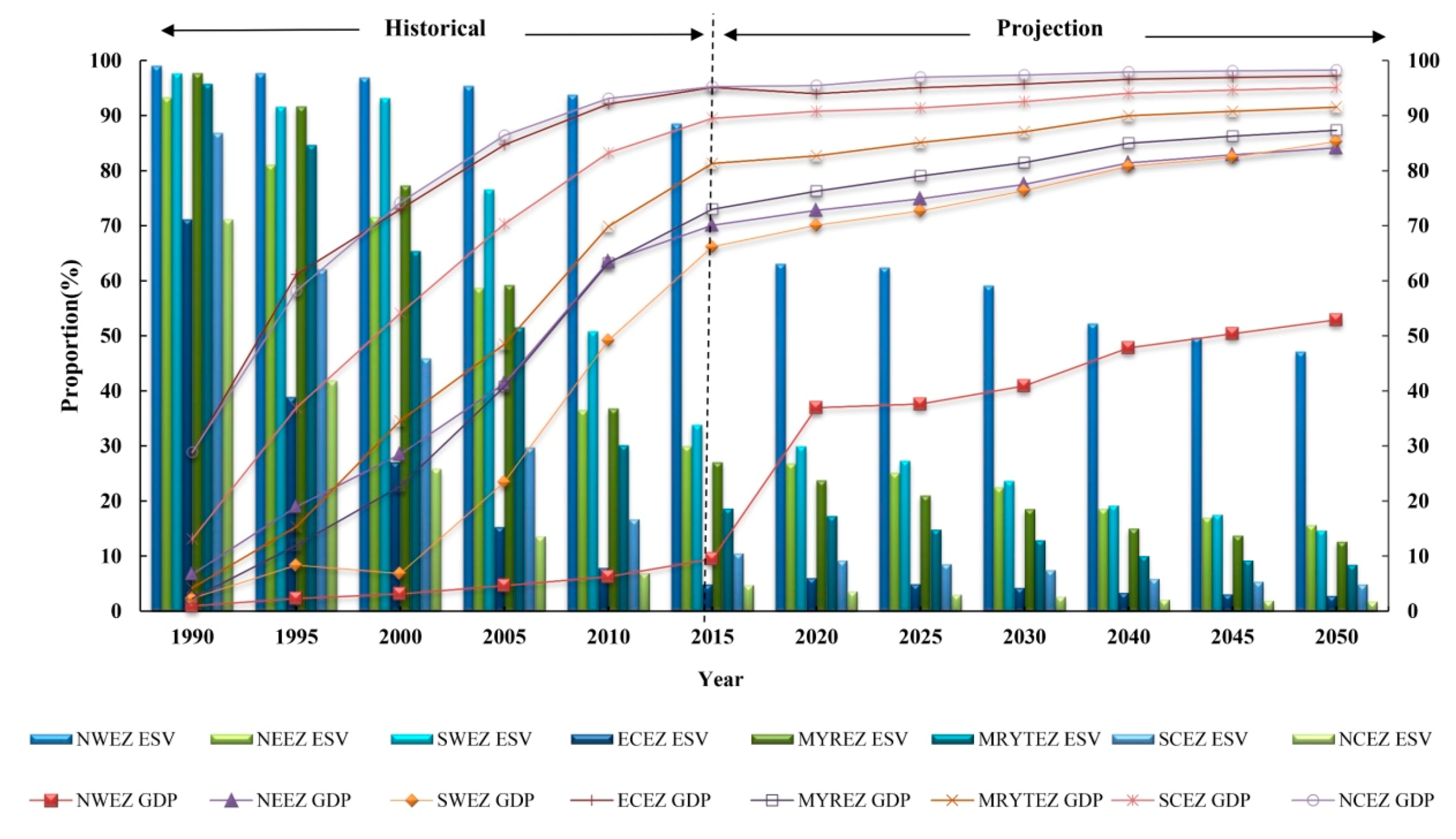
The regional differences in the contributions of GDP and ESV to green GDP were analyzed. The proportion of ESV and GDP in green GDP changed significantly in regions (see Table 10 and Figure 11). In 1990, for most cities in China, the ESV accounted for 80% to 95% of green GDP. However, when it comes to 2015, due to the drastic economic growth in China, the contribution of ESV has been hugely diminished (see Figure 11).

In regions with high green GDP, the contribution of GDP to green GDP was increased gradually, such as for the SCEZ, ECEZ, NCEZ and the MYTREZ. For example, in the NCEZ, the proportion of GDP accounting for the green GDP had a large increase from 28.85% in 1990 to 98.27% to 2050.

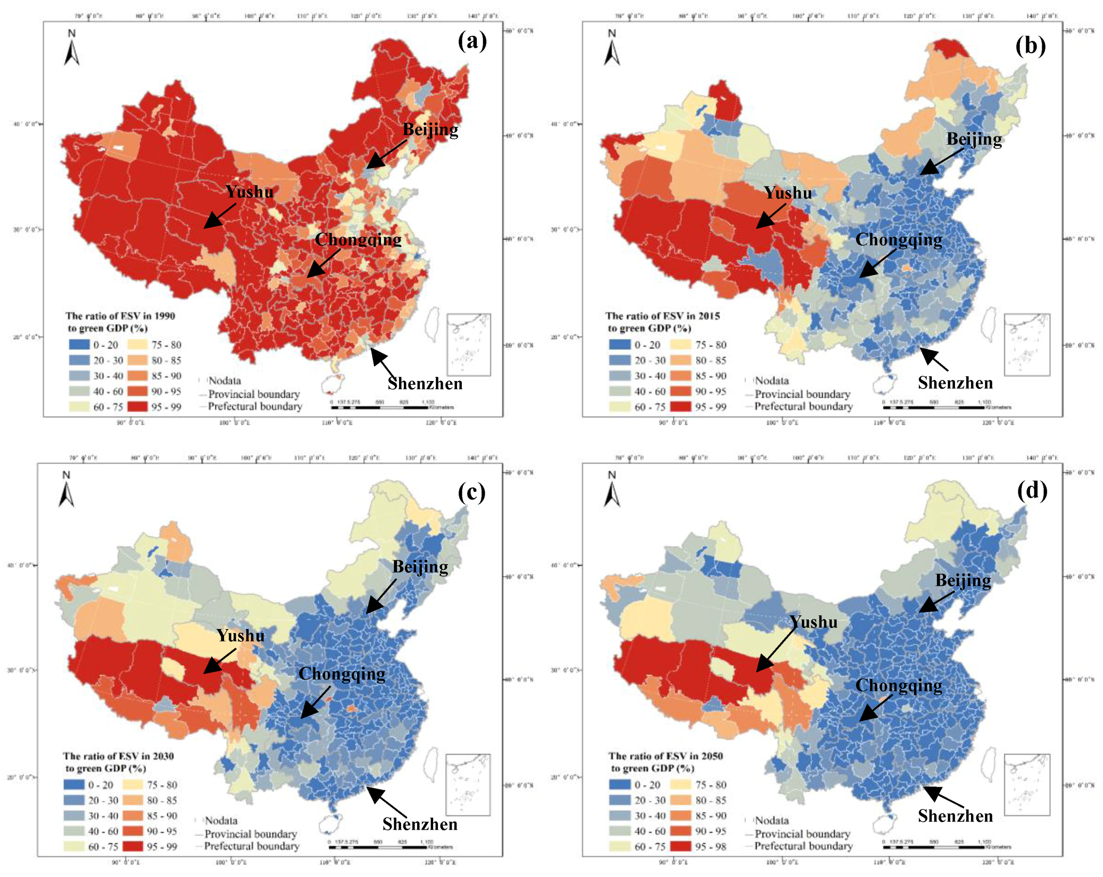
Cities with reducing ESV values and dramatically increasing GDP experienced a huge growth in green GDP, such as Shenzhen, Chongqing and Beijing (see Figure 12). Taking Shenzhen as an example, it demonstrated that the proportion of GDP in green GDP was 98.30%.

However, on the other hand, the green GDP in regions with low GDP was largely dependent on the variation of ESV and the drop in ESV would lead to a direct decrease in green GDP. For example, in the NWEZ, the ESV accounted for 99.06% of green GDP in 1990 and the contribution would drop to 47.10% in 2050. Consider, as an example, Yushu in Qinghai province, the contribution rate of ESV to green GDP of which was 95.20% in 1990 and 92.57% in 2050 and ESV has always occupied a high proportion.

5. Conclusions and Discussion

This study proposed a green GDP accounting and predicting system for prefecture-level cities for China. In the proposed method, we used the coefficient method to measure the ESV according to the output of local agricultural crops and land use patterns; on the other hand, the GDP value was obtained from statistical yearbooks in China. To measure the future green GDP value, we integrated the land use simulation model, CA-Markov, into the green GDP accounting system. The CA-Markov model was used to predict the future land use pattern, which has been taken as input in the coefficient method to measure the future ESV.

The results indicated that the green GDP value experienced a huge increase from 1990 to 2015 and the forecasting green GDP also displayed a dramatic growth from 2020 to 2050. A totally different increase rate has been found in regions of China. High increase rates of green GDP were concentrated in SCEZ, ECEZ and NCEZ, with growth rates of 87.96%, 93.33% and 93.90%, respectively, from 1990 to 2015 and 94.40%, 96.25% and 97.65%, respectively, from 2015 to 2050. However, in NWEZ and SWEZ, the lowest growth rates of 1.09% and 65.59%, respectively, from 1990 and 2015 and 33.56% and 80.92%, respectively, from 2020 to 2050 have been found. Consequently, the spatial differences in green GDP in regions became increasingly serious. The spatial differences of green GDP also have been detected in some other studies. Li and Fang [9] estimated the global ESV and GDP in 2009. According to the maps of global green GDP presented by Li and Fang [10], the coastal areas, such as Zhejiang and Jiangsu provinces, experienced the highest green GDPs—up to 10,000 to 17,299 US dollar per sq.km in 2009. However, in west China, the green GDP ranged from 0 to 200 US dollars per sq.km in 2009.

Meanwhile, the results indicated a dominant contribution of economic development to green GDP. In the ECEZ, NCEZ and SCEZ, the contribution of GDP to green GDP was up to 90%. A high contribution of GDP to green GDP would depress the importance of preserving ESV. On the contrary, in east China, such as Yunfu in Guangdong, Quzhou in Zhejiang and Huaian in Jiangsu, due to the slow economic development, the contributions of GDP to green GDP were merely 31.91%, 43.40% and 43.89% in 2050. In those regions, the green GDP is dependent on preservation of the ESV to a large extent. Being aware of the contribution of ESV to green GDP in different regions can help the government develop different policies for different regions. Li and Ding [13] evaluated the variations of ESV and GDP for Shananxi province from the 1980s to 2010 and found that disparities in GDP were much higher than those of ESV, which is consistent with our results.

The results proposed in this study can facilitate governmental decision making. Huge spatial differences in the future detected by our study would lead to abundant social problems. Being aware of the differences in green GDP, GDP and ESV in regions, a decision maker can determine the hotspots and make policies accordingly to preserve GDP or ESV.

References

- National Bureau of Statistics of China. China Statistical Yearbook; China Statistics Press: Beijing, China, 2016.
- Sun, W.; Miao, Z.; Sun, W.; School, B. Change in the value of ecosystem services of Beijing-Tianjin-Hebei area and its relationship with economic growth. Ecol. Econ. 2015, 31, 59–62. [Google Scholar]
- United Nations, E.C. International Monetary Fund, Organisation for Economic Cooperation and Development; World Bank, System of National Accounts: New York, NY, USA, 1993. [Google Scholar]
- Bartelmus, P. SEEA-2003: Accounting for sustainable development? Ecol. Econ. 2007, 61, 613–616. [Google Scholar] [CrossRef]
- Sutton, P.C.; Costanza, R. Global estimates of market and non-market values derived from nighttime satellite imagery, land cover, and ecosystem service valuation. Ecol. Econ. 2002, 41, 509–527. [Google Scholar] [CrossRef]
- Kunanuntakij, K.; Varabuntoonvit, V.; Vorayos, N.; Panjapornpon, C.; Mungcharoen, T. Thailand green gdp assessment based on environmentally extended input-output model. J. Clean. Prod. 2017, 167, 970–977. [Google Scholar] [CrossRef]
- Lin, W.B.; Yang, J.; Chen, B. Temporal and spatial analysis of integrated energy and environment efficiency in China based on a Green GDP index. Energies 2011, 4, 1376–1390. [Google Scholar] [CrossRef]
- Talberth, J.; Bohara, A.K. Economic openness and green gdp. Ecol. Econ. 2006, 58, 743–758. [Google Scholar] [CrossRef]
- Li, V.; Lang, G. China’s “Green GDP” Experiment and the Struggle for Ecological Modernisation. J. Contemp. Asia. 2010, 40, 44–62. [Google Scholar] [CrossRef]
- Li, G.; Fang, C. Global mapping and estimation of ecosystem services values and gross domestic product: A spatially explicit integration of national ‘green GDP’ accounting. Ecol. Indic. 2014, 46, 293–314. [Google Scholar] [CrossRef]
- Yang, C.; Poon, J.P.H. Regional Analysis of China’s Green GDP. Eur. Geogr. Econ. 2009, 50, 54–563. [Google Scholar] [CrossRef]
- Xu, L.; Bing, Y.; Yue, W. A method of green GDP accounting based on eco-service and a case study of Wuyishan, China. Procedia Environ. Sci. 2010, 2, 1865–1872. [Google Scholar] [CrossRef] [Green Version]
- Li, T.; Ding, Y. Spatial disparity dynamics of ecosystem service values and GDP in Shaanxi Province, China in the last 30 years. PLoS ONE 2017, 12, e0174562. [Google Scholar] [CrossRef] [PubMed]
- Hou, Q.; Zhou, Q. Spatio-temporal relationships between urban growth and economic development: A case study of the Pearl River Delta of China. Asian Geogr. 2012, 29, 57–69. [Google Scholar] [CrossRef]
- Arowolo, A.O.; Deng, X.; Olatunji, O.A.; Obayelu, A.E. Assessing changes in the value of ecosystem services in response to land-use/land-cover dynamics in nigeria. Sci. Total Environ. 2018, 636, 597–609. [Google Scholar] [CrossRef] [PubMed]
- Xu, D.; Ding, X. Assessing the impact of desertification dynamics on regional ecosystem service value in north china from 1981 to 2010. Ecosyst. Serv. 2018, 30, 172–180. [Google Scholar] [CrossRef]
- Anderson, S.J.; Ankor, B.L.; Sutton, P.C. Ecosystem service valuations of south africa using a variety of land cover data sources and resolutions. Ecosyst. Serv. 2017, 27, 173–178. [Google Scholar] [CrossRef]
- Yang, X.; Zheng, X.Q.; Chen, R. A land use change model: Integrating landscape pattern indexes and markov-ca. Ecological Model. 2014, 283, 1–7. [Google Scholar] [CrossRef]
- Halmy, M.W.A.W. Land use/land cover change detection and prediction in the north-western coastal desert of egypt using markov-ca. Appl. Geogr. 2015, 63, 101–112. [Google Scholar] [CrossRef]
- Qing-Sheng, Y.; Xia, L. Integration of multi-agent systems with cellular automata for simulating urban land expansion. Sci. Geogr. Sin. 2017, 27, 542–548. [Google Scholar]
- Kamusoko, C.; Aniya, M.; Adi, B.; Manjoro, M. Rural sustainability under threat in zimbabwe—Simulation of future land use/cover changes in the bindura district based on the markov-cellular automata model. Appl. Geogr. 2009, 29, 435–447. [Google Scholar] [CrossRef]
- Burstedde, C.; Klauck, K.; Schadschneider, A.; Zittartz, J. Simulation of pedestrian dynamics using a two-dimensional cellular automaton. Phys. A Stat. Mech. Appl. 2001, 295, 507–525. [Google Scholar] [CrossRef] [Green Version]
- Kirchner, A.; Schadschneider, A. Simulation of evacuation processes using a bionics-inspired cellular automaton model for pedestrian dynamics. Phys. A Stat. Mech. Appl. 2002, 312, 260–276. [Google Scholar] [CrossRef] [Green Version]
- Barlovic, R.; Santen, L.; Schadschneider, A.; Schreckenberg, M. Metastable states incellular automata for traffic flow. Eur. Phy. J. B. 1998, 5, 793–800. [Google Scholar] [CrossRef]
- Karafyllidis, I.; Thanailakis, A. A model for predicting forest fire spreading using cellular automata. Ecol. Model. 1997, 99, 87–97. [Google Scholar] [CrossRef]
- Tobler, W.R. Cellular geography. In Philosophy in Geography; Gale, S., Olssen, G., Eds.; D. Reidel Publishing Co.: Dortrecht, Holland, 1979; pp. 379–386. [Google Scholar]
- Clarke, K.C.; Gaydos, L.J. Loose-coupling a cellular automaton model and gis: Long-term urban growth prediction for san francisco and washington/baltimore. Int. J. Geogr. Inf. Syst. 1998, 12, 16. [Google Scholar] [CrossRef] [PubMed]
- Li, X.; Yeh, A. Neural-network-based cellular automata for simulating multiple land use changes using gis. Int. J. Geogr. Inf. Syst. 2002, 16, 323–343. [Google Scholar] [CrossRef]
- Etemadi, H.; Smoak, J.M.; Karami, J. Land use change assessment in coastal mangrove forests of iran utilizing satellite imagery and ca–markov algorithms to monitor and predict future change. Environ. Earth Sci. 2018, 77, 208. [Google Scholar] [CrossRef]
- Shafizadeh Moghadam, H.; Helbich, M. Spatiotemporal urbanization processes in the megacity of mumbai, india: A markov chains-cellular automata urban growth model. App. Geogr. 2013, 40, 140–149. [Google Scholar] [CrossRef]
- Xuan, F.H. The coupling development between tourism economy and ecological environment in harbin city. Adv. Mater. Res. 2013, 4, 726–731. [Google Scholar] [CrossRef]
- Department of Rural Surveys, National Bureau of Statistics. China Yearbook of Agricultural Price Survey; China Statistics Press: Beijing, China, 2016.
- Costanza, R.; d’Arge, R.; Groot, R.d.; Farberk, S.; Grasso, M.; Hannon, B.; Limburg, K.; Naeem, S.; Neill, R.V.O.; Paruelo, J.; et al. The value of the world’s ecosystem services and natural capital. Nature 1997, 387, 253–260. [Google Scholar] [CrossRef]
- Xie, G.D.; Zhang, C.X.; Zhang, C.S.; Xiao, Y.; Lu, C.X. The value of ecosystem services in China. Resour. Sci. 2015, 37, 1740–1746. [Google Scholar]
- Hou, X.Y.; Chang, B.; Yu, X.F. Land use change in Hexi corridor based on CA-Markov methods. Trans. Chin. Soc. Agric. Eng. 2004, 20, 286–291. [Google Scholar]
- Sang, L.; Zhang, C.; Yang, J.; Zhu, D.; Yun, W. Simulation of land use spatial pattern of towns and villages based on ca-markov model. Math. Comput. Model. 2011, 54, 938–943. [Google Scholar] [CrossRef]
- Liu, X.P.; Li, X.; Yeh, G.O.; He, J.Q.; Tao, J. Discovery of transition rules for geographical cellular automata by using ant colony optimization. Sci. China 2007, 50, 1578–1588. [Google Scholar] [CrossRef]
- Wang, S.Q.; Zheng, X.Q.; Zang, X.B. Accuracy assessments of land use change simulation based on markov-cellular automata model. Procedia Environ. Sci. 2012, 13, 1238–1245. [Google Scholar] [CrossRef]
- Martinez, I. Rapd-typing of central and eastern north atlantic and western north pacific minke whales, balaenoptera acutorostrata. ICES J. Mar. Sci. 1999, 56, 640–651. [Google Scholar] [CrossRef]
- Kim, J.; Son, S.K.; Son, J.W.; Kim, K.H.; Shim, W.J.; Kim, C.H.; Lee, K.Y. Venting sites along the fonualei and Northeast Lau spreading centers and evidence of hydrothermal activity at an off-axis caldera in the Northeastern Lau Basin. Geochem. J. 2009, 43, 1–13. [Google Scholar] [CrossRef]
- Liu, J.Y.; Ning, J.; Wen, H.; Xu, X.L.; Zhang, S.Y.; Chang, Z.; Li, R.D.; Wu, S.X.; Hu, Y.F.; Du, G.M.; et al. Spatio-temporal patterns and characteristics of land-use change in china during 2010–2015. Acta Geogr. Sin. 2018, 73, 789–802. [Google Scholar]
- Xu, L.Z.; Fang, C.; Feng, C.; Chen, W.; Hua, Y.U.; Huang, X.H.; Zeng, Y.F.; Li, X.; Hong, S.B.; Zhong, X.F. Spatial and temporal variation of near-ground CO concentration in the Eight Economic Regions in China in May and July, 2013. Acta Sci. Circumst. 2014, 34, 1934–1941. [Google Scholar]
- Changchun, F.; Zanrong, Z.; Nana, C. The economic disparities and their spatio-temporal evolution in china since 2000. Geogr. Res. 2015, 34, 234–246. [Google Scholar]
- Zhao, J.F.; Yan, X.D.; Jia, G.S. Simulation of carbon stocks of forest ecosystems in northeast china from 1981 to 2002. Chin. J. Appl. Ecol. 2009, 20, 241–249. [Google Scholar]
- Gichuki, F.N. Makueni district profile: Soil management and conservation, 1989–1998. Drylands Res. Work. Pap. Drylands Res. 2000, 37, 1243–1257. [Google Scholar]
- Landis, J.R.; Koch, G.G. The measurement of observer agreement for categorical data. Biometrics 1977, 33, 159–174. [Google Scholar] [CrossRef] [PubMed]
- Muhammad, R. Detection of land use/land cover changes and urban sprawl in al-khobar, saudi arabia: An analysis of multi-temporal remote sensing data. ISPRS Int. J. Geo-Inf. 2016, 5, 15. [Google Scholar]
Figure 1.
The framework.
Figure 2.
Spatial pattern of UESV: (a) UESV in 1990 and (b) UESV in 2015.
Figure 3.
The spatial growth rate of UESV from 1990 to 2015.
Figure 4.
Suitability maps for different land uses based on binary and continuous values in the CA-Markov model (the red raster indicates the places that are suitable for the specific land use, while the green raster indicates the places that are not suitable for the specific land use): (a) cultivated land, (b) forestland, (c) grassland, (d) waterbody and (e) construction land.
Figure 5.
Spatial distribution of land use: (a) actual land use pattern and (b) prediction of land use change in 2015.
Figure 6.
Spatial pattern of UESV: (a) forecasting the spatial pattern of UESV in 2020 and (b) UESV forecast for 2050.
Figure 7.
Spatial distribution of UGDP in China: (a) UGDP in 1990 and (b) UGDP in 2015.
Figure 8.
The fitting values of the R square relationship and significant P between the UGDP and the time series: (a) R square and (b) significant P.
Figure 9.
Spatial distributions of UGDP in China: (a) UGDP in 2020 and (b) UGDP in 2050.
Figure 10.
National Ugreen GDP map: (a) Ugreen GDP map for 1990, (b) Ugreen GDP map for 1995, (c) Ugreen GDP map for 2020 and (d) Ugreen GDP map for 2050.
Figure 11.
ESV and GDP as a percentage of green GDP from 1990 to 2050.
Figure 12.
The ratio of ESV to green GDP, (a) the ratio of ESV to green GDP in 1990, (b) the ratio of ESV to green GDP in 2015, (c) the ratio of ESV to green GDP in 2030 and (d) the ratio of ESV to green GDP in 2050.