Water allocation analysis of the Zhanghe River basin using the Graph Model for Conflict Resolution with incomplete fuzzy preferences

Abstract

An incomplete fuzzy preference framework for the Graph Model for Conflict Resolution (GMCR) is proposed to handle both complete and incomplete fuzzy preference information. Usually, decision makers’ (DMs’) fuzzy preferences are assumed to be complete fuzzy preference relations (FPRs). However, in real-life situations, due to lack of information or limited expertise in the problem domain, any DM’s preference may be an incomplete fuzzy preference relation (IFPR). An inherent advantage of the proposed framework for GMCR is that it can complete the IFPRs based on additive consistency, which is a special form of transitivity, a common property of preferences. After introducing the concepts of FPR, IFPR, and transitivity, we propose an algorithm to supplement IFPR, that is, to find an FPR that is a good approximation. To illustrate the usefulness of the incomplete fuzzy preference framework for GMCR, we demonstrate it using to a real-world conflict over water allocation that took place in the Zhanghe River basin of China.

1. Introduction

Strategic conflict is common in multiple-participant multiple-objective decision situations [1,2]. To help decision makers (DMs) facing strategic conflicts, many formal methodologies have been proposed, such as game theory [3], metagame analysis [4], conflict analysis [5,6], drama theory [7,8], and the graph model for conflict resolution (GMCR) [9,10]. GMCR is a flexible methodology for systematically modeling and analyzing conflicts, with several advantages [11,12]: first, it can handle any finite number of DMs, each of whom controls any finite number of options; second, it requires only DMs’ relative preferences over feasible states; third, it can deal with both transitive and intransitive preference information, and properly describe reversible and irreversible moves.

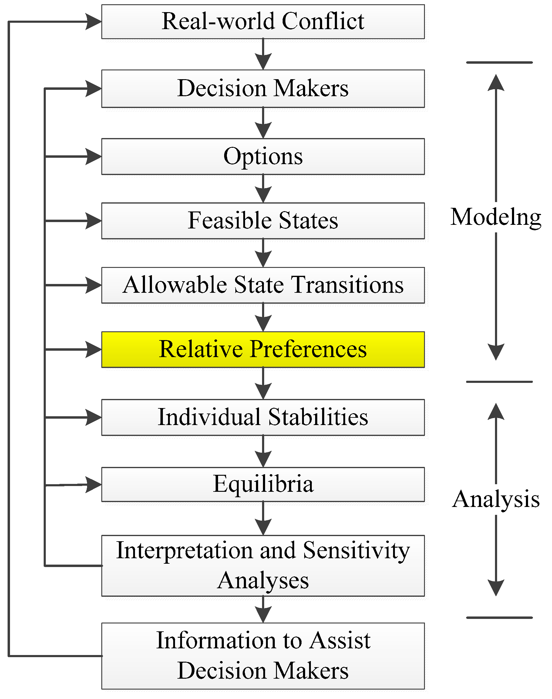
The solid framework of GMCR is based upon several solution concepts that describe human behavior [13,14,15,16,17,18,19]. When GMCR is employed to study a strategic conflict, there are usually two stages (see Figure 1): modeling and analysis [9]. In the modeling stage, DMs and their options are identified; the particular options (courses of action) selected defines each particular state (or scenario). The set of feasible states constitute all of the possible outcomes. GMCR also requires each DM’s relative preferences over the feasible states. In the analysis stage, several stability definitions are used to describe different DM behavior patterns, including Nash stability (R) [20,21], general metarationality (GMR) [22], symmetric metarationality (SMR) [22], and sequential stability (SEQ) [23]. In general, a focal state is stable for a DM under a particular stability definition if it is not advantageous for the DM to move away from the state under that definition. Moreover, a state that is stable for all DMs under a given stability definition is an equilibrium under that definition.

The key input in calculating stability is the DMs’ relative preferences over the states. DMs’ preferences can be given in various forms such as cardinal payoffs (indicating both the ranking and degree of preference) or ordinal preferences (simply ranking the states from most to least preferred). In fact, it is difficult to obtain DMs’ cardinal utilities in a real-life conflict, so it is fortunate that only ordinal rankings are needed to calibrate a graph model. The relative preferences required by GMCR can be expressed using binary relations (‘is strictly preferred to’, $\succ$; and ‘is indifferent to’, $~$). To express a DM’s uncertain preference between two states, Li, et al. [24], proposed a new binary relation ‘is uncertain about’, $U$, and extended four types of stability definitions to graph models with uncertain preference.

A recent addition to GMCR is the fuzzy preference framework, developed using fuzzy preference relations (FPRs) [18]. An FPR is a generalized way of representing both certain and uncertain preferences between two states, using numerical values between 0 and 1, interpreted as degrees of pairwise preferences [25,26,27,28,29,30,31,32]. Within the fuzzy preference framework, four basic stability definitions have been redefined: fuzzy Nash stability (FR), fuzzy general metarationality (FGMR), fuzzy symmetric metarationality (FSMR), and fuzzy sequential stability (FSEQ) [18,19].

However, FPRs are always assumed to be complete (i.e., the degrees of all pairs of states are included) [33]. In practice, the only available information may be an incomplete fuzzy preference relation (IFPR), in which some entries are missing, due to: 1) lack of information and time, or limited expertise [34,35,36]; 2) a large number of states, which may make it impractical to carry out all comparisons required to complete the fuzzy preference matrix [37]; and 3) the inability of a DM to discriminate between states [38,39]. Thus, IFPRs contain more uncertainty, but at the same time may be more widely applicable [35,40].

Motivated by these findings, we propose an incomplete fuzzy preference framework for GMCR. It is not obvious how to incorporate IFPRs into GMCR. Transitivity is a property commonly assumed of preferences: If a state $s_i$ is preferred to state $s_j$ and if $s_j$ is preferred to $s_k$, then state $s_i$ should be preferred to $s_k$. Additive consistency is a specific form of transitivity that applies to fuzzy preferences. The intensity of preference of $s_i$ over $s_k$ equals the sum of the intensities of preference relative to any intermediate state $s_j$. Xu [41] proposed two programming models to find the weighting vector of an IFPR and thereby represent it based on additive consistency. Xu et al. [42] also developed several approaches (normalizing rank aggregation method, logarithmic least squares method [43], and chi-square method [44]) to complete IFPRs. In this study, we propose an algorithm to supplement IFPRs based on additive consistency. To illustrate the usefulness of the incomplete fuzzy preference framework for GMCR, we apply it to a model of a real-world conflict, the water allocation conflict in the Zhanghe River basin (see [45]).

The remainder of this paper is organized as follows: Section 2 provides a basic description of FPRs, IFPRs, transitivity and the supplement method. Section 3 is dedicated to the incomplete fuzzy preference framework for GMCR, including modeling, supplementing, and fuzzy stability analysis. Section 4 presents the application to the Zhanghe River dispute. Section 5 furnishes concluding remarks.

2. Preliminaries

In this section, we introduce some basic terminology and relations that will be used throughout the paper.

2.1. Fuzzy Preference Relations and Transitivity

Let $S=\{s_1,s_2,\dots ,s_n\}$ be a set of feasible states. A fuzzy preference relation over $S$ is a matrix $\Re ={(r_{ij})}_{n\times n}$, where $0\le r_{ij}\le 1$. The membership degree represents the degree of preference of $s_i$ over $s_j$.

Definition 1.

Fuzzy preference relation (FPR) [25,27]: $\Re ={(r_{ij})}_{n\times n}$ is a complete FPR over $S$ if

$$r_{ij}+r_{ji}=1,r_{ii}=0.5,0\le r_{ij}\le 1,\mathrm{for}\mathrm{all}i,j\in N$$

(1)

The interpretations of the values of $r_{ij}$ are as follows:

• (1) $r_{ij}>0.5$ means that it is more likely that state $s_i$ is preferred to state $s_j$ by the DM than the reverse. The larger $r_{ij}$, the more likely $s_i$ is preferred to $s_j$ ($s_i\succ s_j$);
• (2) $r_{ij}<0.5$ means that it is more likely $s_j$ is preferred to state $s_i$ by the DM. The smaller $r_{ij}$, the more likely $s_j$ is preferred to $s_i$ ($s_j\succ s_i$);
• (3) $r_{ij}=1$ means that state $s_i$ is crisply preferred to state $s_j$ by the DM;
• (4) $r_{ij}=0.5$ indicates that DM is indifferent between state $s_i$ and $s_j$ ($s_i\sim s_j$);
• (5) $r_{ij}=0$ means that state $s_i$ is definitely less preferred than state $s_j$ by the DM. Later, we will consider IFPRs, in which some entries are missing.

If $s_i$, $s_j$, and $s_k$ are feasible states and $\Re ={(r_{ij})}_{n\times n}$ is an FPR, then transitivity suggests that if $s_i$ is preferred to state $s_j$ ($r_{ij}\ge \frac{1}{2}$) and $s_j$ is preferred to $s_k$ ($r_{jk}\ge \frac{1}{2}$), then $s_i$ should be preferred to $s_k$ with at least the same intensity.

Definition 2.

Max–min transitivity [27,46]: Let $S=\{s_1,s_2,\dots ,s_n\}$ be a set of feasible states and $\Re ={(r_{ij})}_{n\times n}$ be an FPR over $S$. If $\Re$ satisfies

$$r_{ij}\ge \frac{1}{2}\mathrm{and}{r}_{jk}\ge \frac{1}{2},\mathrm{then}{r}_{ik}\ge \min (r_{ij},r_{jk}),$$

(2)

for all $i$, $j$, and $k$, then $\Re$ is max–min transitive.

For a more specific form of transitivity, consider $r_{ij}-\frac{1}{2}$ to be the intensity of preference of $s_i$ over $s_j$. Then it is reasonable to suppose the intensity of preference of $s_i$ over $s_k$ should be equal to the sum of the intensities of preference relative to an intermediate state $s_j$.

Definition 3.

Additive consistency [27,33,46]: Let $S=\{s_1,s_2,\dots ,s_n\}$ be a set of feasible states and $\Re ={(r_{ij})}_{n\times n}$ be an FPR over $S$. If $\Re$ satisfies

$$r_{ij}\ge \frac{1}{2}\mathrm{and}{r}_{jk}\ge \frac{1}{2},\mathrm{then}\left(r_{ij}-\frac{1}{2}\right)+\left(r_{jk}-\frac{1}{2}\right)=r_{ik}-\frac{1}{2}$$

(3)

for all $i$, $j$, and $k$, then $\Re$ is additively consistent.

Additive consistency is a stronger concept than max–min transitivity [27]. Note that, because of Equation (1), then Equation (3) is equivalent to following equations,

$$r_{ij}+r_{jk}+r_{ki}=1.5$$

(4)

$$r_{ij}=r_{ik}-r_{jk}+0.5$$

(5)

From Definition 3, we obtain the following results:

Theorem 1

[47]. Let $\Re ={(r_{ij})}_{n\times n}$ be a complete FPR. If the diagonal elements are not taken into account, then the sum of all the elements of $\Re$ is $n(n-1)/2$, that is

$${\displaystyle \sum _j^n{\displaystyle \sum _{i=1,i\ne j}^n{r}_{ij}}}={\displaystyle \sum _j^n{\displaystyle \sum _{i=1}^n{r}_{ij}}}-{\displaystyle \sum _{i=1}^n{r}_{ii}}=\frac{n(n-1)}{2}$$

(6)

Theorem 2

[42,47]. If $\Re ={(r_{ij})}_{n\times n}$ is an additively consistent FPR, then there exists a weighting vector $w=(w_1,w_2,\dots ,w_n{)}^T$, where $0\le w_i\le 1$, $i\in N$, ${\displaystyle {\sum }_{i=1}^n{w}_i}=1$, and a positive number $\beta$ such that

$$r_{ij}=0.5+\beta (w_i-w_j),\mathrm{for}\mathrm{all}i,j.$$

(7)

In fact, if $\beta =\frac{n-1}{2}$, then

$$w_i=\frac{{\displaystyle {\sum }_{l=1}^n{r}_{il}-0.5}}{{\displaystyle {\sum }_{i=1}^n{\displaystyle {\sum }_{l=1,l\ne i}^n{r}_{il}}}}=\frac{{\displaystyle {\sum }_{l=1}^n{r}_{il}-0.5}}{\frac{n(n-1)}{2}}$$

(8)

In weighting vector $w={(w_1,w_2,\dots ,w_n)}^T$, $w_i$ reflects the degree of importance of state $s_i$. The larger the value of the weight $w_i$, the more important is state $s_i$. Thus, there is a clear relationship between the original FPR and the weighting vector.

Remark 1.

The use of Equation (8) is called normalizing rank aggregation method. Below, we show how to use Equation (8) to obtain a weighting vector even if FPR is not additively consistent (see [42]).

2.2. Incomplete Fuzzy Preference Relations and Their Completeness

Let $S=\{s_1,s_2,\dots ,s_n\}$ be a set of feasible states. As noted above, an FPR over $S$ may have missing preference entries.

Definition 4.

Incomplete fuzzy preference relation (IFPR) [41]: $\Re ={(r_{ij})}_{n\times n}$ is an IFPR over $S$ if it contains the degrees of preference between some, but not all of the pairs of states of $S$. Each missing entry is denoted by the unknown number “$x_{ij}$”. All other entries are assumed to satisfy Equation (1).

Definition 5.

Additively consistent IFPR [41]: $\Re ={(r_{ij})}_{n\times n}$ is an additively consistent IFPR over $S$ if and only if (iff) $r_{ij}$, $r_{jk}$, and $r_{ik}$ satisfy Equation (3), whenever $r_{ij}$, $r_{jk}$, and $r_{ik}$ are all known.

To supplement an IFPR means to complete it so that the completed IFPR has greatest additive consistency.

Theorem 3

[48,49]. An IFPR $\Re ={(r_{ij})}_{n\times n}$ can be completed if at least $n-1$ independent non-diagonal entries are known, provided that each state is included in a comparison at least once. That is, each of $1,2,\dots ,n$ appears at least once in the subscripts of the known elements of $\Re$.

Sometimes, an IFPR may be inconsistent. Liu, et al. [49] proposed a least square method to find consistent preference relation closest to the IFPR, supplementing the missing entries using $r_{ij}=\beta (w_i-w_j)+0.5$. Thus, for any IFPR $\Re ={(r_{ij})}_{n\times n}$, suppose that $w={(w_1,w_2,\dots ,w_n)}^T$ is the weighting vector. It is reasonable to replace the unknown preference value “$x_{ij}$” in row $i$ and column $j$ of $\Re ={(r_{ij})}_{n\times n}$ with $0.5+\beta (w_i-w_j)$. The auxiliary FPR $\overline{\Re }={({\overline{r}}_{ij})}_{n\times n}$, has

$${\overline{r}}_{ij}=\{\begin{array}{l}{r}_{ij},if{r}_{ij}\ne x_{ij}\\ 0.5+\beta (w_i-w_j),if{r}_{ij}=x_{ij}\end{array}.$$

(9)

If $0\le {\overline{r}}_{ij}\le 1$, $i,j=1,2,\dots ,n$, and $\beta =\frac{n-1}{2}$, the supplement has succeeded. However, an entry ${\overline{r}}_{ij}$ may be outside $[0,1]$. Suppose that ${\overline{r}}_{ij}=-g_{ij}$ or ${\overline{r}}_{ij}=1+g_{ij}$, where $g_{ij}>0$. In such a case, Herrera-Viedma, et al. [46] proposed to transform the matrix $\overline{\Re }={({\overline{r}}_{ij})}_{n\times n}$ into another matrix $\tilde{\Re }={({\tilde{r}}_{ij})}_{n\times n}$, where $g$ is the maximum value of $g_{ij}$ in $\overline{\Re }$.

$${\tilde{r}}_{ij}=\frac{{\overline{r}}_{ij}+g}{1+2g},i,j=1,2,\dots ,n$$

(10)

In order to calculate conveniently, we develop an algorithm for supplementing IFPRs.

Algorithm 1

Input: IFPR $\Re ={(r_{ij})}_{n\times n}$.

Output: Complete FPR $\overline{\Re }={({\overline{r}}_{ij})}_{n\times n}$.

Step 1. Apply Equation (9) to replace formally unknown element “$x_{ij}$” in row $i$ and column $j$ of $\Re$ using $0.5+\beta (w_i-w_j)$, where $\beta =\frac{n-1}{2}$.

Step 2. Utilize the normalizing rank aggregation method to obtain an equation for each weight, $$w_i=\frac{{\displaystyle {\sum }_{j=1,j\ne i}^n{\overline{r}}_{ij}}}{{\displaystyle {\sum }_{i=1}^n{\displaystyle {\sum }_{j=1,j\ne i}^n{\overline{r}}_{ij}}}}=\frac{{\displaystyle {\sum }_{j=1,j\ne i}^n{\overline{r}}_{ij}}}{n(n-1)/2}$$ (11) Now rewrite Equation (11) for i = 1, 2, …, n, as a he system of equations: $$Aw=b$$ (12) where $b$ is a positive n-vector, and $A$ is a real $n\times n$ matrix.

Step 3. Solve Equation (12) to get a weighting vector $w={(w_1,w_2,\dots ,w_n)}^T$. Then, substituting $w_i$ and $w_j$, $i,j\in N$ into Equation (9), obtain a numerical value for “$x_{ij}$” in $\Re$, and let $\overline{\Re }={({\overline{r}}_{ij})}_{n\times n}$.

Step 4. If there are entries ${\overline{r}}_{ij}$ outside $[0,1]$, either ${\overline{r}}_{ij}=-g_{ij}$ or ${\overline{r}}_{ij}=1+g_{ij}$, where $g_{ij}>0$, then transform matrix $\overline{\Re }={({\overline{r}}_{ij})}_{n\times n}$ into matrix $\tilde{\Re }={({\tilde{r}}_{ij})}_{n\times n}$ by using Equation (10), and let $\overline{\Re }=\tilde{\Re }$.

Step 5. Output the complete FPR $\overline{\Re }={({\overline{r}}_{ij})}_{n\times n}$.

Remark 2.

An analogous method for supplementing IFPRs has been proposed by Xu, et al. [47]. However, that method ignores the possibility that some supplemented entries may be outside $[0,1]$, so that the supplemented FPR does not satisfy Equation (1). But Algorithm 1 avoids this situation, as we illustrate with an example.

Example 1.

Suppose an IFPR $\Re$ over $S=\{s_1,s_2,s_3,s_4\}$ as

$$\begin{array}{l}\hspace{1em}\hspace{1em}\hspace{1em}\hspace{1em}\begin{array}{cccc}{s}_1& s_2& s_3& s_4\end{array}\\ \Re =\begin{array}{c}{s}_1\\ s_2\\ s_3\\ s_4\end{array}\left[\begin{array}{cccc}0.5& 0.8& x_{13}& 0.9\\ 0.2& 0.5& 0.8& 0.6\\ x_{31}& 0.2& 0.5& x_{34}\\ 0.1& 0.4& x_{43}& 0.5\end{array}\right]\end{array}.$$

We supplement this IFPR $\Re$ using Algorithm 1:

• Step 1. Replacing each unknown element “$x_{ij}$” appropriately, we construct $\overline{\Re }$ as

  $$\begin{array}{cccccc}& s_1& s_2& s_3& s_4& \\ \overline{\Re }=\begin{array}{c}{s}_1\\ s_2\\ s_3\\ s_4\end{array}[& \begin{array}{c}0.5\\ 0.2\\ 1.5\times (w_3-w_1)+0.5\\ 0.1\end{array}& \begin{array}{c}0.8\\ 0.5\\ 0.2\\ 0.4\end{array}& \begin{array}{c}1.5\times (w_1-w_3)+0.5\\ 0.8\\ 0.5\\ 1.5\times (w_4-w_3)+0.5\end{array}& \begin{array}{c}0.9\\ 0.6\\ 1.5\times (w_3-w_4)+0.5\\ 0.5\end{array}& ]\end{array}.$$
• Step 2. By the normalizing rank aggregation method, we have
  $w_1=\frac{{\displaystyle {\sum }_{j=2}^4{\overline{r}}_{1j}}}{{\displaystyle {\sum }_{i=1}^4{\displaystyle {\sum }_{j=1,j\ne i}^4{\overline{r}}_{ij}}}}=\frac{0.8+1.5(w_1-w_3)+0.5+0.9}{6}=\frac{1.5w_1-1.5w_3+2.2}{6}$,
  $w_2=\frac{{\displaystyle {\sum }_{j=1,j\ne 2}^4{\overline{r}}_{2j}}}{{\displaystyle {\sum }_{i=1}^4{\displaystyle {\sum }_{j=1,j\ne i}^4{\overline{r}}_{ij}}}}=\frac{0.2+0.8+0.6}{6}=\frac{1.6}{6}$,
  $\begin{array}{rr}{w}_3& =\frac{{\displaystyle {\sum }_{j=1,j\ne 3}^4{\overline{r}}_{3j}}}{{\displaystyle {\sum }_{i=1}^4{\displaystyle {\sum }_{j=1,j\ne i}^4{\overline{r}}_{ij}}}}=\frac{1.5(w_3-w_1)+0.5+0.2+1.5(w_3-w_4)+0.5}{6}\hfill \\ & =\frac{-1.5w_1+3w_3-1.5w_4+1.2}{6}\hfill \end{array}$
  $w_4=\frac{{\displaystyle {\sum }_{j=2}^4{\overline{r}}_{4j}}}{{\displaystyle {\sum }_{i=1}^4{\displaystyle {\sum }_{j=1,j\ne i}^4{\overline{r}}_{ij}}}}=\frac{0.1+0.4+1.5(w_4-w_3)+0.5}{6}=\frac{-1.5w_3+1.5w_4+1}{6}$.
  The system can be written as

  $$\left[\begin{array}{cccc}4.5& 0& 1.5& 0\\ 0& 6& 0& 0\\ 1.5& 0& 3& 1.5\\ 0& 0& 1.5& 4.5\end{array}\right]\left[\begin{array}{c}{w}_1\\ w_2\\ w_3\\ w_4\end{array}\right]=\left[\begin{array}{c}2.2\\ 1.6\\ 1.2\\ 1\end{array}\right].$$
• Step 3. The solution of this linear system of equations to is $w_1=0.4667$, $w_2=0.2667$, $w_3=0.0667$, $w_4=0.2$. Using the weighting vector, $w=(0.4667,0.2667,0.0667,0.2{)}^T$, the missing entries in the IFPR are

  $${\overline{r}}_{13}=1.5(w_1-w_3)+0.5=1.1, {\overline{r}}_{31}=1.5(w_3-w_1)+0.5=-0.1,$$

  $${\overline{r}}_{34}=1.5(w_3-w_4)+0.5=0.3, {\overline{r}}_{43}=1.5(w_4-w_3)+0.5=0.7.$$
• Step 4. Entries ${\overline{r}}_{13}$ and ${\overline{r}}_{31}$ lie outside $[0,1]$, where $g_{13}=g_{31}=0.1$. Using Equation (10), we obtain

  $$\begin{array}{cccccc}& s_1& s_2& s_3& s_4& \\ \overline{\Re }=\tilde{\Re }=\begin{array}{c}{s}_1\\ s_2\\ s_3\\ s_4\end{array}[& \begin{array}{c}0.5\\ 0.25\\ 0\\ 0.17\end{array}& \begin{array}{c}0.75\\ 0.5\\ 0.25\\ 0.42\end{array}& \begin{array}{c}1.0\\ 0.75\\ 0.5\\ 0.67\end{array}& \begin{array}{c}0.83\\ 0.58\\ 0.33\\ 0.5\end{array}& ]\end{array}.$$

3. An Incomplete Fuzzy Preference Framework for GMCR

In this section, we first introduce the structure of the graph model and fuzzy stability definitions and then develop the graph model with incomplete fuzzy preference relations.

3.1. Structure of the Graph Model for Conflict Resolution

Let $M=\{1,2,\dots ,m\}$ be the set of DMs. In a graph model, DM $k$’s courses of action are called options, represented by $O_1,O_2,\dots ,O_{n_k}$. An option may or may not be selected in a particular scenario. If the option is selected, it is indicated ‘Y’; otherwise, it is indicated ‘N’. Hence, a state $s$ is an ordered tuple of Ys and Ns, usually written as a column, in which the number of entries is the same as the number of options (over all DMs) in the model. Note that a composite state, which is a group of formally distinct but practically indistinguishable states, is possible; usually such a group is represented as one state using ‘–’ indicating that it does not matter whether a particular option is chosen. All feasible combinations of options constitute the set of feasible states $s_1,s_2,$ $\dots ,s_n$.

The nodes in each DM’s directed graph are the feasible states, denoted $S=\{s_1,s_2,\dots ,s_n\}$. The oriented arcs indicate the possible state-to-state movements controlled by the DM. Note that any move may be reversible or irreversible. The moves controlled by DM $k$ are represented by the set of oriented arcs $A_k$, and DM $k$’s directed graph is given by $D_k=(S,A_k)$. If ${\Re }^k$ denotes DM $k$’s preference relation over the feasible states, a general graph model can be described as

$$\langle M,S,\{(D_k,{\Re }^k):k\in M\}\rangle$$

(13)

3.2. Fuzzy Stability Definitions for GMCR

Definition 6.

Fuzzy relative strength of preference (FRSP) [18,19]: Let ${\Re }^k={(r_{ij}^k)}_{n\times n}$ be DM $k$’s complete FPR. Then, for all $i,j\in N$, $k\in M$, DM $k$’s FRSP of state $s_i$ over $s_j$ is defined as ${\alpha }^k(s_i,s_j)=r_{ij}^k-r_{ji}^k$.

Remark 3.

Note that $-1\le {\alpha }^k(s_i,s_j)\le 1$. ${\alpha }^k(s_i,s_j)=1$ indicates that state $s_i$ is preferred to state $s_j$ by DM $k$; ${\alpha }^k(s_i,s_j)=0$ means that DM is indifferent between state $s_i$ and state $s_j$; ${\alpha }^k(s_i,s_j)=-1$ indicates that state $s_j$ is definitely preferred to state $s_i$ by DM $k$. Moreover, DM $k$’s FRSP over $S$ can be represented by the skew-symmetric matrix ${\alpha }^k={({\alpha }_{ij}^k)}_{n\times n}$.

Definition 7.

Fuzzy satisficing threshold (FST) [18,19]: If DM $k$ would be willing to move from state $s\in S$ to state $s_i\in S$ iff ${\alpha }^k(s_i,s)\ge {\gamma }_k$, then DM $k$’s FST is ${\gamma }_k$ ($0<{\gamma }_k\le 1$).

Remark 4.

The FST is a behavioral parameter representing the DM’s criterion for deciding whether to take advantage of a possible move. Different DMs may have different criteria for choosing states that benefit them, and therefore may even have different FSTs at different times.

Definition 8.

In a graph model $\langle M,S,\{(D_k,{\Re }^k):k\in M\}\rangle$, DM $k$’s reachable list from state $s\in S$ is

$$R_k(s)=\{s_i\in S:(s,s_i)\in A_k\}$$

(14)

Any member of $R_k(s)$ is called a unilateral move for DM $k$ from $s$.

Definition 9.

Fuzzy unilateral improvement (FUI) [18,19]: A state $s_i\in R_k(s)$ is called an FUI for DM $k$ from $s$ iff ${\alpha }^k(s_i,s)\ge {\gamma }_k$.

Definition 10.

Fuzzy unilateral improvement list (FUIL) [18,19]: The set of all FUIs from state $s\in S$ for DM $k$ is called DM $k$’s FUIL from $s$, and is denoted as ${\tilde{R}}_{k,{\gamma }_k}^{+}(s)=\{s_i\in R_k(s):{\alpha }^k(s_i,s)\ge {\gamma }_k\}$. For simplicity, write ${\tilde{R}}_k^{+}(s)={\tilde{R}}_{k,{\gamma }_k}^{+}(s)$.

Definition 11.

Reachable list for a coalition [18,19]: Let $s\in S$, $H\subseteq M$, $H\ne \cancel{Ø}$. Then the reachable list of coalition $H$ from $s$ is $R_H(s)=\{q\in S:thereexists{s}_1,s_2,\dots ,s_{t}suchthat{s}_0=s,s_t=q,and,$ $forj=1,2,\dots ,t,s_j\in R_{k_j}(s_{j-1}),where{k}_j\in H,and,forj>1,k_j\ne k_{j-1}\}$. Any member of $R_H(s)$ is called an UM for coalition $H$ from $s$.

Definition 12.

FUI by a Coalition [18,19]: Let $s\in S$, $H\subseteq M$, $H\ne \cancel{Ø}$. The FUI of coalition $H$ from $s$ is ${\tilde{R}}_H^{+}(s)=\{q\in S:thereexists{s}_1,s_2,\dots ,s_{t}suchthat{s}_0=s,s_t=q,and,forj=1,2,\dots ,t,s_j\in {\tilde{R}}_{k_j}^{+}(s_{j-1}),$ $where{k}_j\in H,and,forj>1,k_j\ne k_{j-1}\}$. Any member of ${\tilde{R}}_H^{+}(s)$ is called an FUI for coalition $H$ from $s$.

In stability analysis, one important task is to determine whether a DM is better to stay at a focal state or to move to another state. Bashar, et al. [18] provide four fuzzy stability definitions to identify possible equilibria in the model. The fuzzy stability definitions for conflict models with more than two DMs are shown in

Table 1. Fuzzy stability definitions.

Stability	Definitions
FR	A state $s\in S$ is FR for DM $k\in M$ iff ${\tilde{R}}_k^{+}(s)=\cancel{Ø}$
FGMR	A state $s\in S$ is FGMR for DM $k\in M$ iff for every $s_1\in {\tilde{R}}_k^{+}(s)$, there exists an $s_2\in R_{M-k}(s_k)$ such that ${\alpha }^k(s_2,s)<{\gamma }_k$
FSMR	A state $s\in S$ is FSMR for DM $k\in M$ iff for every $s_1\in {\tilde{R}}_k^{+}(s)$, there exists an $s_2\in R_{M-k}(s_k)$ such that ${\alpha }^k(s_2,s)<{\gamma }_k$, and ${\alpha }^k(s_3,s)<{\gamma }_k$ for all $s_3\in R_k(s_2)$
FSEQ	A state $s\in S$ is FSEQ for DM $k\in M$ iff for every $s_1\in {\tilde{R}}_k^{+}(s)$, there exists an $s_2\in {\tilde{R}}_{M-k}^{+}(s_k)$ such that ${\alpha }^k(s_2,s)<{\gamma }_k$

. A state that is fuzzy stable for all DMs under a specific fuzzy stability definition is fuzzy equilibrium (FE) under that definition. Of course, fuzzy stability depends on the DMs’ FSTs, given by $\gamma =({\gamma }_1,{\gamma }_2,\dots ,{\gamma }_m)$.

3.3. Graph Model with Incomplete Fuzzy Preference Relations

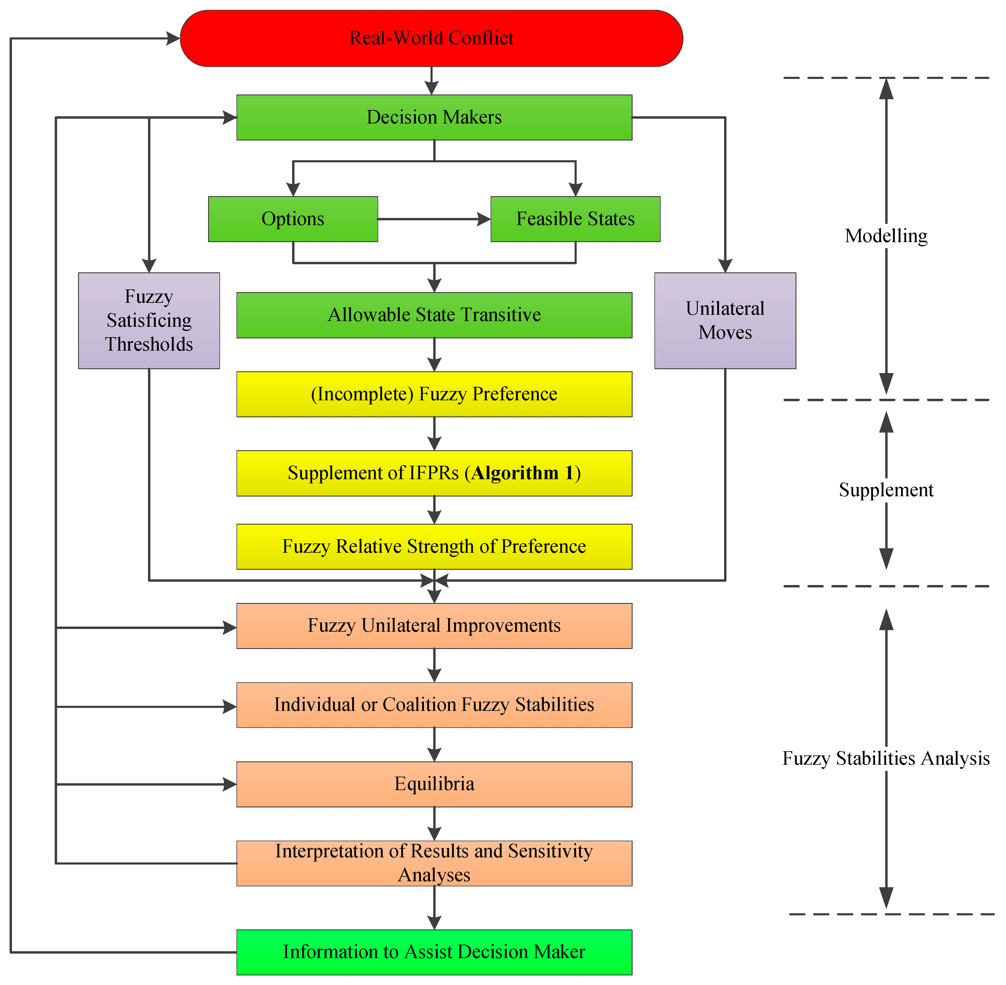
When DMs have complete FPRs, GMCR involves two stages: modeling and (stability) analysis. When one or more DM’s fuzzy preferences are IFPRs, another step, supplementing, must be added. We propose an algorithm for application of GMCR when IFPRs are present. In fact, our algorithm has the advantage of handling both complete and incomplete FPRs. It contains three stages as displayed in Figure 2:

(1)

Modeling stage. Identify the relevant DMs in the real-world conflict under study, specifying their options, determining the feasible states, and establishing their relative preferences over states. Note that DMs’ preferences may be crisp or fuzzy, and if fuzzy, complete or incomplete.

(2)

Supplementing stage. If any preferences are IFPRs, supplement them using Algorithm 1;

(3)

Fuzzy stability analysis stage. Calculate possible equilibria of the model and assess the results.

4. Application to the Zhanghe River Water Allocation Dispute in China

The water allocation conflict in the Zhanghe River basin, studied in [45,50], is a useful case study to illustrate the applicability of the proposed conflict analysis algorithm. In [45], DMs’ preferences are assumed to be crisp. In fact, water allocation is typically a multiple-participant multiple-objective decision problem, and it is difficult to estimate DMs’ crisp preferences or even complete FPRs. So, as a demonstration, we consider in this study that the preference of one of the DMs is an IFPR.

4.1. Conflict Modeling

4.1.1. Background

In China, the Zhanghe River is the main water supply for industrial and agricultural production, and drinking water for Shanxi, Hebei, and Henan provinces. Because of climatic and terrain factors, the distribution of rain in this region is temporally and spatially uneven. With economic development, many larger reservoirs were constructed upstream, many canals built downstream, and a number of hydropower stations were positioned along the river. Unfortunately, water demand now exceeds supply, and many water conflicts took place in the 108.44 km section of the river that serves as the border area of three provinces, Shanxi, Henan, and Hebei, beginning in the 1950s. Shanxi is upstream, where regional water resources are comparatively abundant; it has most of the reservoirs. Hebei and Henan, where regional water resources are lacking, are downstream on the left and right bank, respectively. Since the 1950s, up to 30 large-scale water conflicts have led to economic losses and social unrest in the Zhanghe basin. For instance, during the Spring Festival of 1999, the water infrastructure was sabotaged using explosives by people from both Henan and Hebei. According to reports, water facilities were destroyed, nearly 100 villagers were injured, and about CNY 8,000,000 (USD 1,333,333) in direct economic value was lost [45].

The Zhanghe River Upstream Management Bureau (ZRUMB), which serves the border area of the three provinces and governs the 108.44 km section, has tried many methods to resolve the disputes. For example, ZRUMB encouraged the three provincial governments to reach a new agreement over water releases from the upstream reservoirs in Shanxi Province to meet downstream demands. Both Henan and Hebei cooperated to buy water from Shanxi at a reasonable price, based on the agreement, and ZRUMB successfully organized five transfers over 2002–2005. Positive social and economic benefits of the water transfer across the three provinces were obtained and included [45]: 1) achieving economic benefits, such as supplying water for about 10,000 people, irrigating 27,000 ha of downstream land, and generating more than CNY 40,000,000 (USD 6,666,667) in economic activity; 2) effectively resolving the contradiction between supply and demand of water resources; and 3) demonstrating that market mechanisms can be a breakthrough point to achieve a new water allocation approach. However, the transfer amounts were mostly based on experience and lacked theoretical justification. Reasonable allocation of water in the Zhanghe River basin is now seen as the key to solve the conflict.

4.1.2. DMs and Options

The first step of GMCR is to identify the DMs. As stated above, there are four main DMs: Shanxi, Henan, Hebei, and ZRUMB, which for simplicity, are denoted $Sx$, $Hn$, $Hb$, and $Z$.

Next, the DMs, options must be identified.$Sx$ is located upstream and has comparatively abundant water resources, but it needs water to generate electricity and meet its own development objectives. Water transfer from $Sx$ to $Hn$ and $Hb$ would be an effective way to solve the imbalances between demand and supply. However, water transfers will definitely incur costs, whether in operating the reservoir or dealing with reduced supply, so $Sx$ is reluctant to release more water downstream unless it is compensated. Normally, both $Hn$ and $Hb$ accept the existing agreements, but in the face of decreasing flows or water shortages in irrigation season, the existing agreements do not work well. $Hn$ and $Hb$ have cooperated to buy water from $Sx$, but people in the two provinces have attempted to obtain more water by taking illegal action. As the moderator, $Z$ has tried to facilitate the cooperation of the three provinces to achieve a new water transfer agreement. To summarize, the options of the DMs shown in

Table 2. DMs and options of the Zhanghe River water allocation conflict.

DMs	Options	Explanation
$Sx$	$O_1$: Transfer	Charge for water transfers to downstream provinces
$Hn$	$O_2$: Accept $O_3$: Take action $O_4$: Cooperate with $Hb$	Accept the existing agreements
		Take illegal actions to get more water
		Cooperate with $Hb$ to buy water from $Sx$
$Hb$	$O_5$: Accept	Accept the existing agreements
	$O_6$: Take action	Take illegal actions to get more water
	$O_7$: Cooperate with $Hn$	Cooperate with $Hn$ to buy water from $Sx$
$Z$	$O_8$: Facilitate	Facilitate three provinces to reach new agreement

.

4.1.3. Feasible States

Let ‘Y’ and ‘N’ indicate that an option is taken, or not taken, by the controlling DM. As can be seen from Table 2, there are four DMs and eight options in this water allocation dispute, mathematically, there are $2^8=256$ states. However, many of these 256 states are infeasible, for many reasons. One example is option dependence: $O_4$ can be selected only if $Sx$ is willing to transfer water to downstream (i.e., $O_1$ is selected), and similarly for $O_7$. The 14 feasible states are shown in

Table 3. Feasible states of the Zhanghe River water allocation conflict.

DMs	Options	${\mathit{s}}_1$	${\mathit{s}}_2$	${\mathit{s}}_3$	${\mathit{s}}_4$	${\mathit{s}}_5$	${\mathit{s}}_6$	${\mathit{s}}_7$	${\mathit{s}}_8$	${\mathit{s}}_9$	${\mathit{s}}_{10}$	${\mathit{s}}_{11}$	${\mathit{s}}_{12}$	${\mathit{s}}_{13}$	${\mathit{s}}_{14}$
$Sx$	$O_1$	N	Y	N	Y	Y	N	Y	N	Y	Y	Y	Y	Y	Y
$Hn$	$\{\begin{array}{l}{O}_2\\ O_3\\ O_4\end{array}$	Y N N	Y N N	N Y N	N Y N	N N Y	Y N N	Y N N	N Y N	N Y N	N N Y	Y N N	N Y N	N N Y	N N Y
$Hb$	$\{\begin{array}{l}{O}_5\\ O_6\\ O_7\end{array}$	Y N N	Y N N	Y N N	Y N N	Y N N	N Y N	N Y N	N Y N	N Y N	N Y N	N N Y	N N Y	N N Y	N N Y
$Z$	$O_8$	N	N	N	N	N	N	N	N	N	N	N	N	N	Y

.

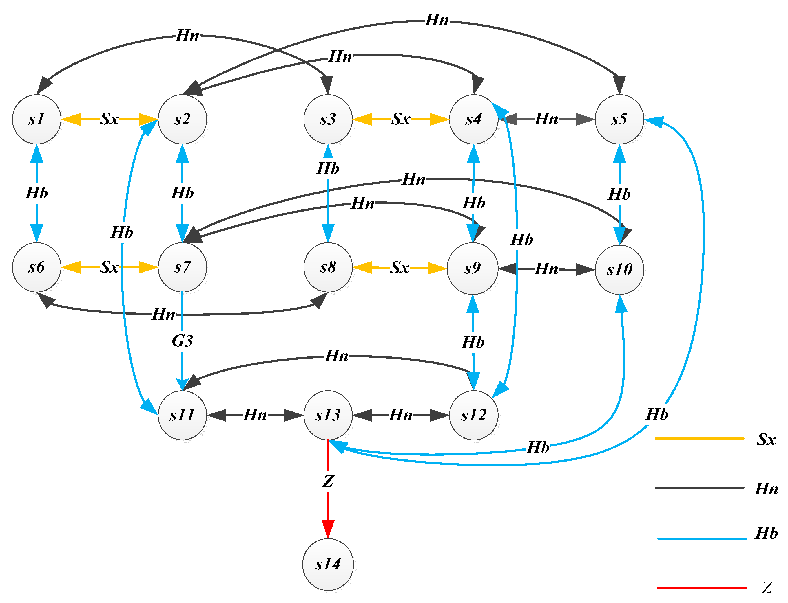
4.1.4. Allowable State Transition

Figure 3 shows the integrated graph of the Zhanghe River water allocation conflict. The nodes of the graph represent feasible states, and the labels on the arcs indicate the controlling DM. The arrowhead(s) on an arc indicate the allowable move directions. Both reversible and irreversible moves are included in this model. For instance, the move between states $s_1$ and $s_2$ by $Sx$ is reversible. However, the move from $s_{13}$ to $s_{14}$ by $Z$ is irreversible.

4.1.5. Relative Preferences

As an administrative agency, $Z$ can mediate (help the negotiators reach a win-win outcome) without being closely connected to the conflict. For $Z$, the ideal situation is that $Hn$ and $Hb$ accept the existing agreement for water resources allocation, enabling it to spend more time and effort on other management activities. Furthermore, $Z$ hopes to promote cooperation between $Hn$ and $Hb$ provided $Sx$ is willing to transfer water downstream and $Hn$ and $Hb$ do not attempt to act illegally. Because their water shortages are becoming serious, $Hn$ and $Hb$ both prefer to have adequate water, especially during the dry season. If $Sx$ agrees to transfer water downstream, $Hn$ and $Hb$ prefer to cooperate with each other. If it is difficult to cooperate, they want $Z$ to mediate. If there is no serious water shortage, they both prefer to accept the existing agreements rather than obtain water illegally. Note that, the preferences of Z, Hn, and Hb over the feasible states are crisp, as in Chu, et al. [45]. They are shown in

Table 4. Preference rankings of $Z$, $Hn$, $Hb$.

DMs	Rankings
$Z$	$s_1$	$s_2$	$s_{13}$	$s_3$	$s_6$	$s_8$	$s_5$	$s_4$	$s_{10}$	$s_7$	$s_{11}$	$s_{12}$	$s_9$	$s_{14}$
$Hn$	$s_{14}$	$s_1$	$s_3$	$s_6$	$s_{13}$	$s_8$	$s_{11}$	$s_{12}$	$s_5$	$s_{10}$	$s_2$	$s_4$	$s_7$	$s_9$
$Hb$	$s_{14}$	$s_1$	$s_6$	$s_3$	$s_{13}$	$s_8$	$s_5$	$s_{10}$	$s_{11}$	$s_{12}$	$s_2$	$s_7$	$s_4$	$s_9$

.

If $Sx$ agrees to transfer water downstream, the compensation it receives can be used not only to maintain water conservation projects, but also to promote the development of a water saving society. However, the cost of the reservoir operations and the price of the transferred water is uncertain; If $Sx$ does not transfer water downstream, its development will be affected, since $Sx$ is adjacent to areas of $Hn$ and $Hb$. Thus, in the Zhanghe River water allocation conflict, $Sx$ is the key to resolving the problem. $Sx$’s preference is quite complicated and as the IFPR (matrix ${\Re }^{Sx}$) is shown in

Table 5. Preference of $Sx$.

$\begin{array}{cccccccccccccccc}& s_1& s_2& s_3& s_4& s_5& s_6& s_7& s_8& s_9& s_{10}& s_{11}& s_{12}& s_{13}& s_{14}& \\ {\Re }^{Sx}=\begin{array}{c}{s}_1\\ s_2\\ s_3\\ s_4\\ s_5\\ s_6\\ s_7\\ s_8\\ s_9\\ s_{10}\\ s_{11}\\ s_{12}\\ s_{13}\\ s_{14}\end{array}(& \begin{array}{c}0.5\\ x_{21}\\ 0.4\\ 1\\ 1\\ 0.3\\ 0.9\\ 0\\ 0.6\\ 0.7\\ 0.8\\ 0.9\\ 1\\ 1\end{array}& \begin{array}{c}{x}_{12}\\ 0.5\\ 0\\ 0.3\\ 0.4\\ 0\\ 0.1\\ 0\\ 0\\ 0\\ 0\\ 0.2\\ 1\\ 1\end{array}& \begin{array}{c}0.6\\ 1\\ 0.5\\ x_{43}\\ 1\\ x_{63}\\ 1\\ 0\\ 0.7\\ 0.8\\ 0.9\\ 1\\ 1\\ 1\end{array}& \begin{array}{c}0\\ 0.7\\ x_{34}\\ 0.5\\ 0.6\\ 0\\ 0.3\\ 0\\ 0\\ 0.1\\ 0.2\\ 0.4\\ 1\\ 1\end{array}& \begin{array}{c}0\\ 0.6\\ 0\\ 0.4\\ 0.5\\ 0\\ 0.2\\ 0\\ 0\\ 0.1\\ x_{11,5}\\ 0.3\\ 1\\ 1\end{array}& \begin{array}{c}0.7\\ 1\\ x_{36}\\ 1\\ 1\\ 0.5\\ x_{76}\\ 0\\ 0.8\\ 0.9\\ 1\\ 1\\ 1\\ 1\end{array}& \begin{array}{c}0.1\\ 0.9\\ 0\\ 0.7\\ 0.8\\ x_{67}\\ 0.5\\ 0\\ 0.2\\ 0.3\\ 0.4\\ 0.6\\ 1\\ 1\end{array}& \begin{array}{c}1\\ 1\\ 1\\ 1\\ 1\\ 1\\ 1\\ 0.5\\ x_{98}\\ 1\\ 1\\ 1\\ 1\\ 1\end{array}& \begin{array}{c}0.4\\ 1\\ 0.3\\ 1\\ 1\\ 0.2\\ 0.8\\ x_{89}\\ 0.5\\ 0.6\\ 0.7\\ 0.8\\ 1\\ 1\end{array}& \begin{array}{c}0.3\\ 1\\ 0.2\\ 0.9\\ 0.9\\ 0.1\\ 0.7\\ 0\\ 0.4\\ 0.5\\ 0.6\\ x_{12,10}\\ 1\\ 1\end{array}& \begin{array}{c}0.2\\ 1\\ 0.1\\ 0.8\\ x_{5,11}\\ 0\\ 0.6\\ 0\\ 0.3\\ 0.4\\ 0.5\\ 0.7\\ 1\\ 1\end{array}& \begin{array}{c}0.1\\ 0.8\\ 0\\ 0.6\\ 0.7\\ 0\\ 0.4\\ 0\\ 0.2\\ x_{10,12}\\ 0.3\\ 0.5\\ 1\\ 1\end{array}& \begin{array}{c}0\\ 0\\ 0\\ 0\\ 0\\ 0\\ 0\\ 0\\ 0\\ 0\\ 0\\ 0\\ 0.5\\ 1\end{array}& \begin{array}{c}0\\ 0\\ 0\\ 0\\ 0\\ 0\\ 0\\ 0\\ 0\\ 0\\ 0\\ 0\\ 0\\ 0.5\end{array}& )\end{array}$

. Specifically, the least preferred situation for $Sx$ is that in which $Hn$ and $Hb$ choose option $O_3$ and $O_6$ (Take action). $Sx$ prefers to select option $O_1$ and prefers that ZRUMB selects option $O_8$ when $Hn$ and $Hb$ choose option $O_4$ and $O_7$ (Cooperation), while $Sx$ has difficulty choosing between $s_3$ and $s_6$, in which either $Hn$ or $Hb$ select ‘Take action’ when $Sx$ does not select option $O_1$ and ZRUMB does not select option $O_8$. Thus, it is appropriate to model $Sx$’s preferences as the IFPR shown in Table 5. For example, the entry in the third row and the sixth column of ${\Re }^{Sx}$ is incomplete, i.e., $Sx$’s preference degree of state $s_3$ over state $s_6$ is unknown; the number 0.6 in the first row and the third column of ${\Re }^{Sx}$ represents the preference degree of state $s_1$ over state $s_3$.

4.2. The Process of Supplementing Incomplete Fuzzy Preference Relations

As previously discussed, if the preference for a DM is an IFPR, the IFPR can be supplemented by using Algorithm 1. Suppose $w={(w_1,w_2,\dots ,w_{14})}^T$ is the weighting vector of the IFPR ${\Re }^{Sx}={(r_{ij})}_{14\times 14}$, the procedure of supplementing the IFPR is as follows:

• Step 1. Apply Equation (9) to replace each unknown element “$x_{ij}$” and construct FPR $\overline{\Re }$.
• Step 2. Use the normalizing rank aggregation method to obtain equations for the weights. The system of equations can be rewritten in the following form:

  $$\left[\begin{array}{cccccccccccccc}84.5& 6.5& 0& 0& 0& 0& 0& 0& 0& 0& 0& 0& 0& 0\\ 6.5& 84.5& 0& 0& 0& 0& 0& 0& 0& 0& 0& 0& 0& 0\\ 0& 0& 84.5& 6.5& 0& 6.5& 0& 0& 0& 0& 0& 0& 0& 0\\ 0& 0& 6.5& 84.5& 0& 0& 0& 0& 0& 0& 0& 0& 0& 0\\ 0& 0& 0& 0& 84.5& 0& 0& 0& 0& 0& 6.5& 0& 0& 0\\ 0& 0& 6.5& 0& 0& 78& 6.5& 0& 0& 0& 0& 0& 0& 0\\ 0& 0& 0& 0& 0& 6.5& 84.5& 0& 0& 0& 0& 0& 0& 0\\ 0& 0& 0& 0& 0& 0& 0& 84.5& 6.5& 0& 0& 0& 0& 0\\ 0& 0& 0& 0& 0& 0& 0& 6.5& 84.5& 0& 0& 0& 0& 0\\ 0& 0& 0& 0& 0& 0& 0& 0& 0& 84.5& 0& 6.5& 0& 0\\ 0& 0& 0& 0& 6.5& 0& 0& 0& 0& 0& 84.5& 0& 0& 0\\ 0& 0& 0& 0& 0& 0& 0& 0& 0& 6.5& 0& 84.5& 0& 0\\ 0& 0& 0& 0& 0& 0& 0& 0& 0& 0& 0& 0& 91& 0\\ 0& 0& 0& 0& 0& 0& 0& 0& 0& 0& 0& 0& 0& 91\end{array}\right]\left[\begin{array}{c}{w}_1\\ w_2\\ w_3\\ w_4\\ w_5\\ w_6\\ w_7\\ w_8\\ w_9\\ w_{10}\\ w_{11}\\ w_{12}\\ w_{13}\\ w_{14}\end{array}\right]=\left[\begin{array}{c}3.9\\ 9.5\\ 3\\ 8.2\\ 8.9\\ 2.6\\ 6.5\\ 0.5\\ 3.7\\ 5.4\\ 6.4\\ 7.4\\ 12\\ 13\end{array}\right]$$
• Step 3. Solving, we obtain the weighting vector $w={(0.0377,0.1095,0.285,0.0948,0.1001,0.0247,0.0750,0.0026,0.0436,0.0575,0.0680,0.0832,0.1319,0.1429)}^{\mathrm{T}}$. Then, substituting into Equation (9), we obtain the unknown preferences ${\overline{r}}_{12}=0.03$, ${\overline{r}}_{21}=0.97$, ${\overline{r}}_{34}=0.07$, ${\overline{r}}_{43}=0.93$, ${\overline{r}}_{36}=0.52$, ${\overline{r}}_{63}=0.48$, ${\overline{r}}_{5,11}=0.71$, ${\overline{r}}_{21}=0.29$, ${\overline{r}}_{67}=0.17$, ${\overline{r}}_{76}=0.83$, ${\overline{r}}_{89}=0.23$, ${\overline{r}}_{98}=0.77$, ${\overline{r}}_{10,12}=0.33$, ${\overline{r}}_{12,10}=0.67$.
• Step 4. No entries in ${\overline{\Re }}^{Sx}={({\overline{r}}_{ij})}_{n\times n}$ are outside $[0,1]$, so we have the complete FPR

  $$\begin{array}{cccccccccccccccc}& s_1& s_2& s_3& s_4& s_5& s_6& s_7& s_8& s_9& s_{10}& s_{11}& s_{12}& s_{13}& s_{14}& \\ {\overline{\Re }}^{Sx}=\begin{array}{c}{s}_1\\ s_2\\ s_3\\ s_4\\ s_5\\ s_6\\ s_7\\ s_8\\ s_9\\ s_{10}\\ s_{11}\\ s_{12}\\ s_{13}\\ s_{14}\end{array}(& \begin{array}{c}0.5\\ 0.97\\ 0.4\\ 1\\ 1\\ 0.3\\ 0.9\\ 0\\ 0.6\\ 0.7\\ 0.8\\ 0.9\\ 1\\ 1\end{array}& \begin{array}{c}0.03\\ 0.5\\ 0\\ 0.3\\ 0.4\\ 0\\ 0.1\\ 0\\ 0\\ 0\\ 0\\ 0.2\\ 1\\ 1\end{array}& \begin{array}{c}0.6\\ 1\\ 0.5\\ 0.93\\ 1\\ 0.48\\ 1\\ 0\\ 0.7\\ 0.8\\ 0.9\\ 1\\ 1\\ 1\end{array}& \begin{array}{c}0\\ 0.7\\ 0.07\\ 0.5\\ 0.6\\ 0\\ 0.3\\ 0\\ 0\\ 0.1\\ 0.2\\ 0.4\\ 1\\ 1\end{array}& \begin{array}{c}0\\ 0.6\\ 0\\ 0.4\\ 0.5\\ 0\\ 0.2\\ 0\\ 0\\ 0.1\\ 0.29\\ 0.3\\ 1\\ 1\end{array}& \begin{array}{c}0.7\\ 1\\ 0.52\\ 1\\ 1\\ 0.5\\ 0.83\\ 0\\ 0.8\\ 0.9\\ 1\\ 1\\ 1\\ 1\end{array}& \begin{array}{c}0.1\\ 0.9\\ 0\\ 0.7\\ 0.8\\ 0.17\\ 0.5\\ 0\\ 0.2\\ 0.3\\ 0.4\\ 0.6\\ 1\\ 1\end{array}& \begin{array}{c}1\\ 1\\ 1\\ 1\\ 1\\ 1\\ 1\\ 0.5\\ 0.77\\ 1\\ 1\\ 1\\ 1\\ 1\end{array}& \begin{array}{c}0.4\\ 1\\ 0.3\\ 1\\ 1\\ 0.2\\ 0.8\\ 0.23\\ 0.5\\ 0.6\\ 0.7\\ 0.8\\ 1\\ 1\end{array}& \begin{array}{c}0.3\\ 1\\ 0.2\\ 0.9\\ 0.9\\ 0.1\\ 0.7\\ 0\\ 0.4\\ 0.5\\ 0.6\\ 0.67\\ 1\\ 1\end{array}& \begin{array}{c}0.2\\ 1\\ 0.1\\ 0.8\\ 0.71\\ 0\\ 0.6\\ 0\\ 0.3\\ 0.4\\ 0.5\\ 0.7\\ 1\\ 1\end{array}& \begin{array}{c}0.1\\ 0.8\\ 0\\ 0.6\\ 0.7\\ 0\\ 0.4\\ 0\\ 0.2\\ 0.33\\ 0.3\\ 0.5\\ 1\\ 1\end{array}& \begin{array}{c}0\\ 0\\ 0\\ 0\\ 0\\ 0\\ 0\\ 0\\ 0\\ 0\\ 0\\ 0\\ 0.5\\ 1\end{array}& \begin{array}{c}0\\ 0\\ 0\\ 0\\ 0\\ 0\\ 0\\ 0\\ 0\\ 0\\ 0\\ 0\\ 0\\ 0.5\end{array}& )\end{array}$$

4.3. Stability Analysis

This section describes the stability analysis of the Zhanghe River water allocation conflict model. To carry out a fuzzy stability analysis means to apply the fuzzy stability definitions to identify states with high degrees of stability. In order to demonstrate how the FSTs of DMs influence fuzzy stabilities, the DMs’ FSTs are set as follows: (1) ${\gamma }_{Sx}=0.3$; (2) ${\gamma }_{Sx}=0.6$; (3) ${\gamma }_{Sx}=0.9$. Note that in each case ${\gamma }_Z={\gamma }_{Hn}={\gamma }_{Hb}=1$, since the preferences of $Z$, $Hn$, and $Hb$ are crisp. The fuzzy equilibrium results are listed in

Table 6. Fuzzy equilibrium analysis results.

FE	Fuzzy equilibrium states
	${\gamma }_Z={\gamma }_{Hn}={\gamma }_{Hb}=1,$ ${\gamma }_{Sx}=0.3$	${\gamma }_Z={\gamma }_{Hn}={\gamma }_{Hb}=1,$ ${\gamma }_{Sx}=0.6$	${\gamma }_Z={\gamma }_{Hn}={\gamma }_{Hb}=1,$ ${\gamma }_{Sx}=0.9$
FR	$s_{13}$, $s_{14}$	$s_{13}$, $s_{14}$	$s_{13}$, $s_{14}$
FGMR	$s_1$, $s_3$, $s_5$, $s_6$, $s_{10}$, $s_{11}$, $s_{12}$, $s_{13}$, $s_{14}$	$s_1$, $s_3$, $s_5$, $s_6$, $s_8$, $s_{10}$, $s_{11}$, $s_{12}$, $s_{13}$, $s_{14}$	$s_1$, $s_3$, $s_5$, $s_6$, $s_8$, $s_{10}$, $s_{11}$, $s_{12}$, $s_{13}$, $s_{14}$
FSMR	$s_1$, $s_3$, $s_5$, $s_6$, $s_{10}$, $s_{11}$, $s_{12}$, $s_{13}$, $s_{14}$	$s_1$, $s_3$, $s_5$, $s_6$, $s_8$, $s_{10}$, $s_{11}$, $s_{12}$, $s_{13}$, $s_{14}$	$s_1$, $s_3$, $s_5$, $s_6$, $s_8$, $s_{10}$, $s_{11}$, $s_{12}$, $s_{13}$, $s_{14}$
FSEQ	$s_3$, $s_{13}$, $s_{14}$	$s_3$, $s_8$, $s_{13}$, $s_{14}$	$s_1$, $s_3$, $s_6$, $s_8$, $s_{13}$, $s_{14}$

.

As is clear from Table 6: states $s_{13}$, $s_{14}$ have a high degree of stability because they are FEs under all four fuzzy stability definitions for each of the three sets of FSTs. When ${\gamma }_Z={\gamma }_{Hn}={\gamma }_{Hb}=1,{\gamma }_{Sx}=0.6$ and ${\gamma }_Z={\gamma }_{Hn}={\gamma }_{Hb}=1,{\gamma }_{Sx}=0.9$, state $s_8$ is an FE under FGMR, FSMR, and FSEQ. In fact, when $Sx$’s FSTs are increased, $Sx$ has no FUI from state $s_8$. When ${\gamma }_Z={\gamma }_{Hn}={\gamma }_{Hb}=1,{\gamma }_{Sx}=0.9$, states $s_1$ and $s_6$ are found to be FE under FSEQ; for state $s_6$, increasing of $Sx$’s FST means that $Sx$ has no FUI from state $s_6$; for state $s_1$, when $Sx$’s FST increases from 0.6 to 0.9, $Sx$ becomes more conservative so that the benefit is not enough to motivate leaving $s_1$.

The status quo state of the Zhanghe River water allocation conflict model was state $s_1$: $Sx$ is reluctant to transfer water ($O_1$ is not selected); both $Hn$ and $Hb$ accept existing agreements ($O_2$ and $O_5$); and $Z$ does not facilitate the three provinces to reach a new agreement ($O_8$ is not selected). When the shortage of water is serious, $Hn$ and $Hb$ prefer to take illegal actions to obtain water ($O_3$ and $O_6$), and thereby shift the model to state $s_8$. As a neighboring province of $Hn$ and $Hb$, $Sx$ prefers that the downstream provinces live peacefully with each other. If $Sx$ can benefit from selling water to them at a suitable price, it will agree to transfer water ($O_1$), and cause a transition from state $s_8$ to $s_9$.

When $Sx$ agrees to transfer water, $Hn$ and $Hb$ prefer to cooperate with each other to buy water. Therefore $Hn$ and $Hb$ choose cooperation ($O_4$ and $O_7$) instead of taking illegal action ($O_3$ and $O_6$). Ideally, the conflict will reach the equilibrium at state $s_{13}$. However, for cooperation, the services of $Z$ are sometimes needed to reach an agreement at which $Sx$ transfers water downstream for charge. Finally, with the transition from state $s_9$ to $s_{14}$, the conflict is resolved. The evolution of this model can be seen in

Table 7. Process of state transition in the Zhanghe River water allocation conflict.

DM	Options	${\mathit{s}}_1$		${\mathit{s}}_8$		${\mathit{s}}_9$		${\mathit{s}}_{13}$	or	${\mathit{s}}_{14}$
$Sx$	O1: Transfer	N		N	$\to$	Y		Y		Y
$Hn$	O2: Accept	Y	$\to$	N		N		N		N
	O3: Take action	N	$\to$	Y		Y	$\to$	N	$\to$	N
	O4: Cooperate with $Hb$	N		N		N	$\to$	Y	$\to$	Y
$Hb$	O5: Accept	Y	$\to$	N		N		N		N
	O6: Take action	N	$\to$	Y		Y	$\to$	N	$\to$	N
	O7: Cooperate with $Hn$	N		N		N	$\to$	Y	$\to$	Y
$Z$	O8: Facilitate	N		N		N		N	$\to$	Y

.

5. Conclusions

The results of the formal investigation the water conflict in the Zhanghe River basin using the incomplete fuzzy preference framework for GMCR reveal that transferring water from Shanxi to Henan and Hebei is an effective way to resolve this conflict. The new methodology is a more general approach for decision making under strategic conflict compared with the both crisp and fuzzy graph models, and contains three stages: modeling, supplementing, and fuzzy stability analysis. Furthermore, the incomplete fuzzy graph model offers the analyst sufficient flexibility to handle strategic conflicts even when the DMs’ fuzzy preferences are incomplete, and thereby makes the investigation of strategic conflicts more realistic. In the Zhanghe basin model, most of these possibilities are short-term solutions, not long-term stable solutions as water ecosystems, the participation of government and marketplace, and other factors, may change. In fact, only by ensuring that water conservation projects in the upstream province can facilitate water transportation is there likely to be a lasting resolution to downstream water conflicts in the future.

This study still has some deficiencies. For instance, the crisp and fuzzy graph models were designed to deal with both transitive and intransitive relative preferences, and the incomplete fuzzy graph model considers only fuzzy preferences that satisfy additive consistency such as those in [29,41,42]. In addition, each DM is treated as an independent individual, without considering the complex power relations between them. In the near future, the incomplete fuzzy preference framework of GMCR might also be integrated with other developments, such as coalition analysis [51], status quo analysis [2], scale analysis [52], and power asymmetry analysis [53] to provide a deeper analysis of the water conflict in the Zhanghe River basin.

References

- Hipel, K.W.; Kilgour, D.M.; Bashar, M.A. Fuzzy preferences in multiple participant decision making. Sci. Iran. 2011, 18, 627–638. [Google Scholar] [CrossRef]
- Li, K.W.; Hipel, K.W.; Kilgour, D.M.; Noakes, D. Integrating uncertain preferences into status quo analysis with applications to an environmental conflict. Group Decis. Negot. 2005, 14, 461–479. [Google Scholar] [CrossRef]
- Von Neumann, J.; Morgenstern, O. Theory of Games and Economic Behavior, 3rd ed.; Princeton University Press: Princeton, NJ, USA, 1953. [Google Scholar]
- Howard, N. Paradoxes of Rationality: Theory of Metagama and Political Behavior; MIT Press: Cambridge, MA, USA, 1971. [Google Scholar]
- Fraser, N.M.; Hipel, K.W. Solving complex conflicts. IEEE Trans. Syst. Man Cybern. Syst. 1979, 9, 805–816. [Google Scholar] [CrossRef]
- Xu, Y.J.; Zhang, W.C.; Wang, H.M. A conflict-eliminating approach for emergency group decision of unconventional incidents. Knowl.-Based Syst. 2015, 83, 92–104. [Google Scholar] [CrossRef]
- Howard, N. Drama theory and its relation to game theory. Part 1: Dramatic resolution vs. Rational solution. Group Decis. Negot. 1994, 3, 187–206. [Google Scholar] [CrossRef]
- Howard, N. Drama theory and its relation to game theory. Part 2: Formal model of the resolution process. Group Decis. Negot. 1994, 3, 207–235. [Google Scholar] [CrossRef]
- Kilgour, D.M.; Hipel, K.W.; Fang, L.P. The graph model for conflicts. Automatica 1987, 23, 41–55. [Google Scholar] [CrossRef]
- Fang, L.P.; Hipel, K.W.; Kilgour, D.M. Conflict models in graph form: Solution concepts and their interrelationships. Eur. J. Oper. Res. 2007, 41, 86–100. [Google Scholar] [CrossRef]
- Fang, L.P.; Hipel, K.W.; Kilgour, D.M. Interactive Decision Making: The Graph Model for Conflict Resolution; Wiley: New York, NY, USA, 1993. [Google Scholar]
- Xu, H.Y.; Hipel, K.W.; Kilgour, D.M.; Fang, L.P. Conflict Resolution Using the Graph Model: Strategic Interactions in Competition and Cooperation; Springer: Cham, Switzerland, 2018. [Google Scholar]
- Hipel, K.W.; Meister, D.B. Conflict analysis methodology for modelling coalition in multilateral negotiations. Inf. Decis. Technol. Amsterdam 1994, 19, 85–103. [Google Scholar]
- Fang, L.P.; Hipel, K.W.; Kilgour, D.M.; Peng, X.Y. A decision support system for interactive decision making—Part II: analysis and output interpretation. IEEE Trans. Syst. Man Cybern. Part C Appl. Rev. 2003, 33, 56–66. [Google Scholar] [CrossRef]
- Inohara, T. Consensus building and the graph model for conflict resolution. In Proceedings of the 2010 IEEE International Conference on Systems, Man and Cybernetics, Istanbul, Turkey, 10–13 October 2010; pp. 2841–2846. [Google Scholar]
- Kuang, H.B.; Bashar, M.A.; Hipel, K.W.; Kilgour, D.M. Grey-based preference in a graph model for conflict resolution with multiple decision makers. IEEE Trans. Syst. Man Cybern. Syst. 2015, 45, 1254–1267. [Google Scholar] [CrossRef]
- Kilgour, D.M.; Hipel, K.W. The graph model for conflict resolution: past, present, and future. Group Decis. Negot. 2005, 14, 441–460. [Google Scholar] [CrossRef]
- Bashar, M.A.; Hipel, K.W.; Kilgour, D.M. Fuzzy preferences in a two-decision maker graph model. In Proceedings of the 2010 IEEE International Conference on Systems, Man and Cybernetics, 2010 IEEE International Conference on Systems, Man and Cybernetics, Istanbul, Turkey, 10–13 October 2010; pp. 2964–2970. [Google Scholar]
- Bashar, M.A.; Kilgour, D.M.; Hipel, K.W. Fuzzy preferences in the graph model for conflict resolution. IEEE Trans. Fuzzy Syst. 2012, 20, 760–770. [Google Scholar] [CrossRef]
- Nash, J.F. Equilibrium points in n-person games. Proc. Natl. Acad. Sci. USA 1950, 36, 48–49. [Google Scholar] [CrossRef] [PubMed]
- Nash, J.F. Non-cooperative games. Ann. Math. 1951, 54, 286–295. [Google Scholar] [CrossRef]
- Howard, N. Dilemmas and sure things. Science 1973, 180, 595–596. [Google Scholar]
- Fraser, N.M.; Hipel, K.W. Conflict Analysis: Models and Resolutions; North-Holland: Amsterdam, The Netherlands, 1984; pp. 972–973. [Google Scholar]
- Li, K.W.; Hipel, K.W.; Kilgour, D.M.; Fang, L.P. Stability definitions for 2-player conflict models with uncertain preferences. In Proceedings of the IEEE International Conference on Systems, Man and Cybernetics, Yasmine Hammamet, Tunisia, 6–9 October 2002. [Google Scholar]
- Orlovsky, S.A. Decision-making with a fuzzy preference relation. Fuzzy Sets Syst. 1978, 1, 155–167. [Google Scholar] [CrossRef]
- Wu, Z.B.; Xu, J.P. A concise consensus support model for group decision making with reciprocal preference relations based on deviation measures. Fuzzy Sets Syst. 2012, 206, 58–73. [Google Scholar] [CrossRef]
- Tanino, T. Fuzzy preference orderings in group decision making. Fuzzy Sets Syst. 1984, 12, 117–131. [Google Scholar] [CrossRef]
- Xu, Y.J.; Patnayakuni, R.; Wang, H.M. The ordinal consistency of a fuzzy preference relation. Inf. Sci. 2013, 224, 152–164. [Google Scholar] [CrossRef]
- Xu, Y.J.; Li, K.W.; Wang, H.M. Distance-based consensus models for fuzzy and multiplicative preference relations. Inf. Sci. 2013, 253, 56–73. [Google Scholar] [CrossRef]
- Xu, Y.J.; Wu, N.N. A two-stage consensus reaching model for group decision making with reciprocal fuzzy preference relations. Soft Comput. 2018. [Google Scholar] [CrossRef]
- Xu, Y.J.; Herrera, F. Visualizing and rectifying different inconsistencies for fuzzy reciprocal preference relations. Fuzzy Sets Syst. 2019, 362, 85–109. [Google Scholar] [CrossRef]
- Xu, Y.J.; Wang, Q.Q.; Cabrerizo, F.J.; Herrera-Viedma, E. Methods to improve the ordinal and multiplicative consistency for reciprocal preference relations. Appl. Soft Comput. 2018, 67, 479–493. [Google Scholar] [CrossRef]
- Chiclana, F.; Herrera-Viedma, E.; Alonso, S.; Herrera, F. Cardinal consistency of reciprocal preference relations: a characterization of multiplicative transitivity. IEEE Trans. Fuzzy Syst. 2009, 17, 14–23. [Google Scholar] [CrossRef]
- Chiclana, F.; Herrera-Viedma, E.; Alonso, S. A note on two methods for estimating missing pairwise preference values. IEEE Trans. Syst. Man Cybern. Part B 2009, 39, 16–28. [Google Scholar] [CrossRef] [PubMed]
- Xu, Y.J.; Chen, L.; Herrera, F.; Wang, H.M. Deriving the priority weights from incomplete hesitant fuzzy preference relations in group decision making. Knowl.-Based Syst. 2016, 99, 71–78. [Google Scholar] [CrossRef]
- Xu, Y.J.; Gupta, J.N.D.; Wang, H.M. The ordinal consistency of an incomplete reciprocal preference relation. Fuzzy Sets Syst. 2014, 246, 62–77. [Google Scholar] [CrossRef]
- Fedrizzi, M.; Giove, S. Incomplete pairwise comparison and consistency optimization. Eur. J. Oper. Res. 2007, 183, 303–313. [Google Scholar] [CrossRef]
- Xu, Z.S. On method for uncertain multiple attribute decision making problems with uncertain multiplicative preference information on alternatives. Fuzzy Optim. Decis. Mak. 2005, 4, 131–139. [Google Scholar] [CrossRef]
- Alonso, S.; Chiclana, F.; Herrera, F.; Herrera-Viedma, E.; Alcalá-Fdez, J.; Porcel, C. A consistency-based procedure to estimate missing pairwise preference values. Int. J. Intell. Syst. 2008, 23, 155–175. [Google Scholar] [CrossRef]
- Wu, N.N.; Xu, Y.J.; Hipel, K.W. The graph model for conflict resolution with incomplete fuzzy reciprocal preference relations. Fuzzy Sets Syst. 2018. [Google Scholar] [CrossRef]
- Xu, Z.S. Goal programming models for obtaining the priority vector of incomplete fuzzy preference relation. Int. J. Approx. Reason. 2004, 36, 261–270. [Google Scholar] [CrossRef]
- Xu, Y.J.; Da, Q.L.; Liu, L.H. Normalizing rank aggregation method for priority of a fuzzy preference relation and its effectiveness. Int. J. Approx. Reason. 2009, 50, 1287–1297. [Google Scholar] [CrossRef]
- Xu, Y.J.; Patnayakuni, R.; Wang, H.M. Logarithmic least squares method to priority for group decision making with incomplete fuzzy preference relations. Appl. Math. Model. 2013, 37, 2139–2152. [Google Scholar] [CrossRef]
- Xu, Y.J.; Chen, L.; Li, K.W.; Wang, H.M. A chi-square method for priority derivation in group decision making with incomplete reciprocal preference relations. Inf. Sci. 2015, 306, 166–179. [Google Scholar] [CrossRef]
- Chu, Y.; Hipel, K.W.; Fang, L.P.; Wang, H.M. Systems methodology for resolving water conflicts: the Zhanghe River water allocation dispute in China. Int. J. Water Resour. D. 2015, 31, 106–119. [Google Scholar] [CrossRef]
- Herrera-Viedma, E.; Herrera, F.; Chiclana, F.; Luque, M. Some issues on consistency of fuzzy preference relations. Eur. J. Oper. Res. 2004, 154, 98–109. [Google Scholar] [CrossRef]
- Xu, Y.J.; Da, Q.L.; Wang, H.M. A note on group decision-making procedure based on incomplete reciprocal relations. Soft Comput. 2008, 12, 515–521. [Google Scholar] [CrossRef]
- Herrera-Viedma, E.; Chiclana, F.; Herrera, F.; Alonso, S. Group decision-making model with incomplete fuzzy preference relations based on additive consistency. IEEE Trans. Syst. Man Cybern. Part B 2007, 37, 176–189. [Google Scholar] [CrossRef]
- Liu, X.W.; Pan, Y.W.; Xu, Y.J.; Yu, S. Least square completion and inconsistency repair methods for additively consistent fuzzy preference relations. Fuzzy Sets Syst. 2012, 198, 1–19. [Google Scholar] [CrossRef]
- Xu, Y.J.; Cabrerizo, F.J.; Herrera-Viedma, E. A consensus model for hesitant fuzzy preference relations and its application in water allocation management. Appl. Soft Comput. 2017, 58, 265–284. [Google Scholar] [CrossRef]
- Kilgour, D.M.; Hipel, K.W.; Fang, L.P.; Peng, X.Y. Coalition analysis in group decision support. Group Decis. Negot. 2001, 10, 159–175. [Google Scholar] [CrossRef]
- Withanachchi, S.S.; Houdret, A.; Nergui, S.; Ejarque Gonzalez, E.; Tsogtbayar, A.; Ploeger, A. (Re)configuration of Water Resources Management in Mongolia: A Critical Geopolitical Analysis; Kassel University Press: Kassel, Germany, 2015. [Google Scholar]
- Yu, J.; Kilgour, D.M.; Hipel, K.W.; Zhao, M. Power asymmetry in conflict resolution with application to a water pollution dispute in China. Water Resour. Res. 2016, 51, 8627–8645. [Google Scholar] [CrossRef]
Figure 1.
The general conflict analysis process (Kilgour, et al. [9]).
Figure 2.
An algorithm for applying GMCR with incomplete fuzzy preference.
Figure 3.
Integrated graph of the Zhanghe River water allocation conflict.