Microgrid Planning Considering the Supply Adequacy of Critical Loads under the Uncertain Formation of Sub-Microgrids

Abstract

A microgrid can be partitioned into several autonomous sub-microgrids in case of multiple faults in natural disasters. How to guarantee the supply adequacy of critical loads in sub-microgrids is a problem that should be considered at the planning stage. This paper proposes a microgrid planning model considering the supply adequacy of critical loads under the uncertain formation of sub-microgrids. The proposed model minimizes the total cost during the project life, which includes the construction cost and operation cost for the candidate distributed energy resources (DERs). The supply adequacy of critical loads in sub-microgrids is taken into account in the model. As we only know the critical load areas, the locations of switches which divide the microgrid into sub-microgrids are unknown at the planning stage. Considering this uncertainty, the microgrid planning issue is finally formulated as a robust model against the worst formation of sub-microgrids. The developed model is tested on two systems: IEEE 33-bus and 123-bus distribution systems. Simulation indicates (1) the proposed method is more robust than deterministic strategy as critical load loss is intolerable in sub-microgrids; (2) the investment cost is the same with that of the deterministic case when the number of sub-microgrids is within two.

1. Introduction

Microgrid is a kind of controllable distribution system with distributed energy resources (DERs) and loads. Due to their significant advantages of controllability and flexibility, microgrids have grown rapidly in recent years. Generally, a microgrid is interconnected with the utility grid through the point of common coupling (PCC). However, it can also break away from the utility grid and operate as an autonomous microgrid in case there is a fault in the PCC. However, in extreme conditions involving hurricanes, thunderstorms, and blizzards, the distribution system may suffer from multiple faults and be split into several isolated sub-systems. In this situation, some microgrids where critical-load loss is intolerable should have the ability to form several autonomous sub-microgrids in case of multiple faults. The sub-microgrid can at least satisfy the power supply of critical loads within it. Therefore, how to guarantee the supply adequacy of those critical loads within the sub-microgrids is also a challenge at the planning stage. Theoretically, more DERs will definitely guarantee the supply adequacy of those loads. However, it may incur a high investment. How to compromise between the economy and the power supply adequacy is not an easy task. To overcome those obstacles, effective microgrid planning models are necessary to be developed considering the supply adequacy of critical loads within possible sub-microgrids.

In the relevant literature, extensive research has been carried out on the optimal operation and planning of microgrids. A bidding strategy for a DER aggregator in the day-ahead market is proposed in Reference [1]. An optimal operation strategy of DERs to reduce the energy cost and environmental impact model is proposed in Reference [2]. However, References [1,2] focus on the concerns of bidding strategy or operation strategy of a microgrid, while the construction costs of DERs should be taken into account for a microgrid planning problem. In contrast, Reference [3] makes a long-term planning of microgrids using a game theoretical approach. In Reference [4], a bi-level island microgrid planning model considering the constructions of photovoltaic arrays, wind turbines, diesel generators, and compressed air energy storage systems is presented. However, the model is a deterministic optimization model. Recent studies tend to take the uncertainty into account using robust, stochastic, or chance constrained models [5,6,7,8]. Reference [5] presents a robust microgrid planning model considering the uncertainties of loads, renewable power, and market prices. The optimal planning of a new class of microgrids, provisional microgrid, is solved by the same method in Reference [6]. Considering the uncertainty of renewable source, an optimal DER placement model in microgrids based on robust optimization is proposed in Reference [7]. Reference [8] describes the microgrid planning problem as a stochastic chance-constrained programming model. One category of studies focuses on the multi-objective optimization of microgrid planning [9,10,11]. Reference [9] proposes a generalized double shell multi-objective framework to optimally design a microgrid system with glow-worm optimization algorithm to solve it. A Multi-objective Substrate Layers Coral Reefs Optimization algorithm is proposed in [10] to decide the optimal placement of generation and the topology of a microgrid. Reference [11] develops a multi-objective coordinated planning model of active-reactive power resources based on the probabilistic load flow. A few papers integrate the heat and cooling resources into the microgrid planning models [12,13]. In Reference [12], the optimal locations, capacity sizes, and types of DERs including combined heat and power systems are studied, and the particle swarm optimization algorithm is adopted to solve the problem. Reference [13] investigates the sizing and management of heating/cooling systems in the context of smart grid with high penetration of renewable energy. Several researches integrate the reliability criterion into the microgrid planning model [14,15]. In Reference [14], a master-slave objective function is developed considering the economic efficiency, environmental restrictions, and reliability improvement. Reference [15] uses reliability criterion to determine the optimal size and location of a mix of distributed generation candidate technologies in a microgrid. The studies mentioned above are all aimed at a single microgrid, some papers consider the coordination of multi-microgrids for their great flexibility [16,17]. Reference [16] proposes a framework for the cooperative planning of renewable generations in several interconnected microgrids, and it demonstrates the overall system cost can be reduced compared to the non-cooperative planning system. Reference [17] applies a probabilistic minimal cut-set-based iterative methodology to the optimal planning of interconnection among microgrids with variable renewable energy resources. The economy, reliability, and uncertainty are all considered in the model. Recently, resilient operation and planning of microgrid are gaining more and more attention to deal with extreme conditions [18,19,20,21,22,23,24,25]. Many microgrids are able to form several autonomous sub-microgrids in case of multiple faults and then restore the loads gradually. To ensure the critical loads after outages occur, sectionalized microgrids are formed with local CHP plants to satisfy maximum self-adequacy in Reference [18]. A microgrid restoration model that considers the three-phase network to represent unbalanced distribution networks is presented in Reference [19]. Reference [20] extends an electricity based microgrid to a multiple energy carrier microgrid, and it proposes a resilient operation model considering multiple disruptions within the microgrid. References [18,19,20] all refer to resilient operation of microgrids. Reference [21] formulates a bi-level optimization model to transform the distribution system with DERs into several autonomous microgrids. Reference [22] also develops an approach to cluster the distribution system into a set of sub-microgrids with self-adequacy. In [23], an approach is proposed by forming multiple microgrids to restore critical loads from the power outage after natural disasters. References [21,22,23] are all associated with resilient formation of sub-microgrids. A planning framework for a hybrid ac-dc isolated system composed of a number of interconnected zones is demonstrated in Reference [24]. Reference [25] presents a flexible network optimal planning model of an autonomy microgrid to improve the flexibility of the planning model.

As can be seen from the relevant literature, many studies such as References [3,4] construct the microgrid planning models with a single objective or multiple objectives in islanded mode or interconnected mode. A few papers such as References [5,8] consider the uncertainties of loads, renewable generation and market prices. Methods such as stochastic optimization, robust optimization, chance-constrained optimization are used to handle the uncertainty. Recently, more and more papers consider the expansion of microgrids considering the formation of multiple sub-microgrids owing to their resilient characteristics in case of power outage such as References [18,19,20,21,22,23,24,25]. However, most of those papers assume the site and number of DERs are fixed. The investment cost of DERs is not fully considered. In addition, the sub-microgrids are usually predetermined. Therefore, to determine the site and number of DERs, a microgrid planning model is proposed in this paper considering the economy of the project and the supply adequacy of critical loads under the uncertain formation of sub-microgrids. In conclusion, the main contributions are shown as follows:

(1)

A DER planning model of an interconnected microgrid considering the supply adequacy of critical loads within sub-microgrids is proposed. In addition to considering the investment and operation cost in interconnected mode, the supply adequacy of critical loads within sub-microgrids in islanded mode is also considered.

(2)

The uncertain formation of sub-microgrids is formulated in this paper. The areas of sub-microgrids are not predetermined at the planning stage, and only the critical loads are known. The possible switches to divide the microgrid into sub-microgrids are considered as variables to model the uncertainty. It is able to form several sub-microgrids according to the position of the critical loads.

(3)

A robust microgrid planning model is developed, which is able to optimize the number and site of DERs against the worst realization of sub-microgrids. An algorithm based on the column-and-constraint generation algorithm is also developed. Test indicates that the arrangement of DERs demonstrates a good robust characteristic. However, it may not necessarily sacrifice the economy.

This paper is organized as follows: The proposed model is presented in Section 2. The developed algorithm to solve the model is demonstrated in Section 3. Two microgrid cases are studied in Section 4, and finally, conclusions are drawn in Section 5.

2. Proposed Microgrid Planning Model

In this section, the basic microgrid planning problem is modeled firstly. After that, the model is extended by introducing the constraints for supply adequacy of sub-microgrids. Considering the uncertain formation of sub-microgrids, the model is comprehensive. Finally, the robust microgrid planning model and the compact form are presented, and it is solved by the column-and-constraint generation algorithm.

2.1. Basic Microgrid Planning Model

The most important issue of a planning problem is the economy of the project. The total cost of the microgrid project consists of construction cost and operation cost. Therefore, the objective of microgrid planning is commonly to minimize the overall cost during the life cycle period of the project. As the life cycle of a microgrid lasts for years, the overall cost during the years is reduced to that in one single year by converting it to the present-worth value. The objective expression of the microgrid planning model is represented as Equation (1). In the objective, the first term represents the construction cost of distributed generators (DGs) such as micro turbines and fuel cells, assuming that the construction cost of DGs is proportional to their capacity, and the present-worth coefficient is used to multiply it for evaluating in terms of discounted cost. The second term is the construction cost of renewable energy resources including wind turbines (WTs) and photovoltaics (PVs). The third term is the construction cost of battery storage systems (BSs). Particularly, the capital cost of BSs is divided into two parts, which are proportional to the maximum capacity and discharging power of BSs, respectively. The remaining items are the annual operating cost of the microgrid. Considering that WTs and PVs can generate without fuel, the operating cost of WTs and PVs are assumed to be zero. The fourth term is the fuel cost of DGs. Assume that the microgrid can buy or sell power from or to the grid. Then the fifth term represents the purchase and sale cost for power exchange with the grid. Specifically, the grid power is negative when the microgrid sells power to the main grid. The sixth term is the penalty cost for load curtailment. Insufficient power supply may cause load loss, and the curtailed consumers should be paid for loss of load.

$$\begin{array}{ll}f=\min & {\displaystyle \sum _{i\in G}{K}_{g,i}^{}{I}_{g,i}^{}{\overline{P}}_{g,i}^{}{x}_{g,i}^{}}+{\displaystyle \sum _{i\in W}{K}_{w,i}^{}{I}_{w,i}^{}{\overline{P}}_{w,i}^{}{x}_{w,i}^{}}+{\displaystyle \sum _{i\in B}{K}_{b,i}^{}(I_{b,i}^P{\overline{P}}_{b,i}^{}+I_{b,i}^E{\overline{E}}_{b,i}^{})x_{b,i}^{}}+\\ & {\displaystyle \sum _d{\displaystyle \sum _h{\displaystyle \sum _{i\in G}{\rho }_{g,i}^{}{p}_{g,i,d,h}^{}}}}+{\displaystyle \sum _d{\displaystyle \sum _h{\rho }_{gd+}^{}{p}_{gd+,d,h}^{}}}-{\rho }_{gd-}^{}{p}_{gd-,d,h}^{}+{\displaystyle \sum _d{\displaystyle \sum _h{\rho }_{lc}^{}{p}_{lc,d,h}^{}}}\end{array}$$

(1)

In the objective function, the capital construction cost of DERs is converted to annual value by multiplying the present-worth coefficient, which is defined as follows:

$$K_{y,i}^{}=\frac{r{(1+r)}^{T_{y,i}^{}}}{{(1+r)}^{T_{y,i}^{}}-1}\forall y\in G,W,B$$

(2)

where T_y,i is the lifespan of the ith device y. Accordingly, the annual operational costs should be the accumulative sum of the daily operational cost in a year. As some days in the year demonstrate similar characteristics, several days with different characteristics are selected as typical days to represent all the days to reduce the computation.

In view of the lack of resources such as financial budgets, the maximum construction number of DGs, BSs is limited as indicated in Equations (3) and (4). Similarly, the maximum construction number of WTs and PVs is also constrained by restrictions such as spatial limits, as implied in (5).

$$0\le {\displaystyle \sum _{i\in G}{x}_{g,i}^{}}\le \left|G\right|$$

(3)

$$0\le {\displaystyle \sum _{i\in B}{x}_{b,i}^{}}\le \left|B\right|$$

(4)

$$0\le {\displaystyle \sum _{i\in W}{x}_{w,i}^{}}\le \left|W\right|$$

(5)

As one DER cannot locate at multiple buses in the microgrid, the state of the DER is equal to the aggregated sum of the location indicators, as shown in Equations (6) to (8). If the DER is installed, only one of the location indicators is active; otherwise, no location indicator is active.

$$x_{g,i}^{}={\displaystyle \sum _{j\in N}{x}_{g,i,j}}\forall i\in G$$

(6)

$$x_{b,i}^{}={\displaystyle \sum _{j\in N}{x}_{b,i,j}}\forall i\in B$$

(7)

$$x_{w,i}^{}={\displaystyle \sum _{j\in N}{x}_{w,i,j}}\forall i\in W$$

(8)

Equation (9) represents the power balance of the microgrid. The total power output of DGs, WTs, PVs, BSs plus the power from the utility grid and the curtailed load equal the electrical load. The power from the utility grid can be negative depending on its flowing direction, and it is limited by its maximum transfer capacity, as shown in Equation (10). The curtailed load should not overstep the current load Equation (11). The power output of DG should be within its lower and upper bounds, as indicated in Equation (12).

$${\displaystyle \sum _{i\in G}{p}_{g,i,d,h}}+{\displaystyle \sum _{i\in W}{p}_{w,i,d,h}}+{\displaystyle \sum _{i\in B}(p_{b+,i,d,h}-p_{b-,i,d,h})}+p_{gd+,d,h}-p_{gd-,d,h}+p_{lc,d,h}=P_{ld,d,h}\forall d,\forall h$$

(9)

$$0\le p_{gd+,d,h},p_{gd-,d,h}\le {\overline{P}}_{gd}\forall d,\forall h$$

(10)

$$0\le p_{lc,d,h}\le P_{ld,d,h}\forall d,\forall h$$

(11)

$$0\le p_{g,i,d,h}\le {\overline{P}}_{g,i}{x}_{g,i}\forall i\in G,\forall d,\forall h$$

(12)

Equation (13) describes the energy storage of BS. The varied energy of BS is equal to the difference between the charging and discharging power with respective efficiency. The discharging power, charging power, and the energy stored in the BS, are constrained by their capacity limits, as specified in Equations (14), (15), (16), (17) indicates the energy balance of BS, namely, the stored energy at the end of the scheduling period is required to be the initial level so as to prepare for the scheduling in the next period.

$$e_{b,i,d,h}=e_{b,i,d,h-1}-p_{b+,i,d,h}/{\eta }_{b+}+p_{b-,i,d,h}{\eta }_{b-}\forall i\in B,\forall d,\forall h$$

(13)

$$0\le p_{b+,i,d,h}\le {\overline{P}}_{b,i}{x}_{b,i}\forall i\in B,\forall d,\forall h$$

(14)

$$0\le p_{b-,i,d,h}\le {\overline{P}}_{b,i}{x}_{b,i}\forall i\in B,\forall d,\forall h$$

(15)

$${\underset{\_}{E}}_{b,i}\le e_{b,i,d,h}\le {\overline{E}}_{b,i}\forall i\in B,\forall d,\forall h$$

(16)

$$e_{b,i,d,H}=E_{b,i,d,0}\forall i\in B,\forall d$$

(17)

If renewable energy resources are deployed, the power generation will be simulated using a typical daily generation curve; otherwise, the generation is zero, as implied in Equation (18).

$$p_{w,i,d,h}=P_{w,i,d,h}{x}_{w,i}\forall i\in W,\forall d,\forall h$$

(18)

Noteworthily, the basic model is founded in the context of interconnected mode. However, as we know, the microgrid can operate in autonomous mode. Furthermore, some resilient microgrids can form several autonomous sub-microgrids when multiple outages occur in extreme conditions. The focus of this paper is the planning of resilient microgrids. In this situation, priority should be given to the supply of critical loads. How to guarantee the supply adequacy of critical loads within sub-microgrids should be considered at the planning stage. Therefore, the constraints for maintaining the power supply of critical loads within sub-microgrids are to be developed.

2.2. Supply Adequacy of Critical Loads

In a microgrid, the power injection at each bus is the difference between the cumulative power output of located DERs and the load. Assume only DGs can generate reactive power. Then, the active and reactive power injections of buses are shown in Equations (19) and (20), respectively. In addition, the power output of DERs is limited by the placement state. Only placed DERs can generate power, as specified in Equations (21) to (25).

$${\tilde{p}}_{in,j}={\displaystyle \sum _{i\in G}{\tilde{p}}_{g,i,j}}+{\displaystyle \sum _{i\in B}({\tilde{p}}_{b+,i,j}-{\tilde{p}}_{b-,i,j})}+{\displaystyle \sum _{i\in W}{\tilde{p}}_{w,i,j}}-{\tilde{P}}_{ld,j}\hspace{1em}\forall j\in N$$

(19)

$${\tilde{q}}_{in,j}={\displaystyle \sum _{i\in G}{\tilde{q}}_{g,i,j}}-{\tilde{Q}}_{ld,j}\forall j\in N$$

(20)

$$0\le {\tilde{p}}_{g,i,j}\le {\overline{P}}_{g,i}{x}_{g,i,j}\forall i\in G,\forall j\in N$$

(21)

$$0\le {\tilde{q}}_{g,i,j}\le {\overline{Q}}_{g,i}{x}_{g,i,j}\forall i\in G,\forall j\in N$$

(22)

$$0\le {\tilde{p}}_{b+,i,j}\le {\overline{P}}_{b,i}{x}_{b,i,j}\forall i\in B,\forall j\in N$$

(23)

$$0\le {\tilde{p}}_{b-,i,j}\le {\overline{P}}_{b,i}{x}_{b,i,j}\forall i\in B,\forall j\in N$$

(24)

$$0\le {\tilde{p}}_{w,i,j}\le {\overline{P}}_{w,i}{x}_{w,i,j}\forall i\in W,\forall j\in N$$

(25)

For sub-microgrids, the linearized DistFlow model is used to formulate the power flow constraints [24], which are expressed as Equations (26) to (32). Equations (26) and (27) denote the active and reactive power balance at the buses. Equations (28) and (29) characterize the voltage relation between the two terminal buses of a branch. Note that c_i,j is the switch state of branch (i,j), and M is a big number. If the switch of a branch is closed, namely c_i,j = 1, the voltage difference between the two terminal buses of a branch is limited by power flow formulation; otherwise c_i,j = 0, the voltage difference can be arbitrary. Similarly, if the switch of a branch is closed, the power flow is constrained; otherwise, there is no power flow between the two terminal buses of the branch, as shown in Equations (30) and (31). The voltage limits are given in Equation (32).

$${\tilde{p}}_{in,j}={\displaystyle \sum _{i\in \pi (j)}{\tilde{p}}_{i,j}}-{\displaystyle \sum _{k\in \sigma (j)}{\tilde{p}}_{j,k}}\forall j\in N$$

(26)

$${\tilde{q}}_{in,j}={\displaystyle \sum _{i\in \pi (j)}{\tilde{q}}_{i,j}}-{\displaystyle \sum _{k\in \sigma (j)}{\tilde{q}}_{j,k}}\forall j\in N$$

(27)

$${\tilde{v}}_i-{\tilde{v}}_j-({\tilde{p}}_{i,j}{R}_{i,j}+{\tilde{q}}_{i,j}{X}_{i,j})\ge -M(1-c_{i,j})\forall (i,j)\in L$$

(28)

$${\tilde{v}}_i-{\tilde{v}}_j-({\tilde{p}}_{i,j}{R}_{i,j}+{\tilde{q}}_{i,j}{X}_{i,j})\le M(1-c_{i,j})\forall (i,j)\in L$$

(29)

$$-{\overline{P}}_{i,j}{c}_{i,j}\le {\tilde{p}}_{i,j}\le {\overline{P}}_{i,j}{c}_{i,j}\forall i,j\in L$$

(30)

$$-{\overline{Q}}_{i,j}{c}_{i,j}\le {\tilde{q}}_{i,j}\le {\overline{Q}}_{i,j}{c}_{i,j}\forall i,j\in L$$

(31)

$${\underset{\_}{V}}_i\le {\tilde{v}}_i\le {\overline{V}}_i\forall i\in N$$

(32)

As mentioned above, c_i,j is the switch state of branch (i,j), and it is introduced to identify the area of a sub-microgrid. If the area of a sub-microgrid is predetermined, c_i,j will also be determined. If the power supply in the sub-microgrids is adequate, constraints Equations (19) to (32) will always hold. Otherwise, the model may be infeasible. If the area of a sub-microgrid is not predetermined, c_i,j will be a variable to be optimized.

To avoid constructing two DERs at one bus, at most one DER is allowed to place at one bus, as shown in Equation (33).

$${\displaystyle \sum _{i\in G}{x}_{g,i,j}}+{\displaystyle \sum _{i\in B}{x}_{b,i,j}}+{\displaystyle \sum _{i\in W}{x}_{w,i,j}}\le 1\forall j\in N$$

(33)

2.3. The Uncertain Formation of Sub-Microgrids

At the planning stage, we are not sure how many sub-microgrids may form and how large the area of the sub-microgrid is. However, the critical load areas are sure. Our goal is to make sure these loads are adequately supplied by DERs within the sub-microgrids. To describe the uncertain formation of sub-microgrids, a new uncertainty set is developed.

Since there are critical loads in the network, the switch of branches connected to those loads should be closed in the sub-microgrids. In addition, some branches are always closed. Except those branches, the other branches’ switches may divide the whole microgrid into several sub-microgrids. Therefore, the constraints of the switch states of branches can be expressed as:

$$\begin{array}{l}{c}_{i,j}=1\forall (i,j)\in L_0\\ 0\le c_{i,j}\le 1\forall (i,j)\in L\backslash L_0\end{array}$$

(34)

where L₀ is the predetermined closed branches set in the microgrid. The switch state of those branches equals to 1, otherwise it is an arbitrary integer between 0 and 1.

A microgrid is usually a radial distribution system, and the sub-microgrids are also radial. According to the graph theory [26], when a radial graph is partitioned into several radial sub-graphs, the number of branches is equal to the number of nodes minus the number of sub-graphs, as indicated in Equation (35).

$${\displaystyle \sum _{(i,j)\in L}{c}_{i,j}}=|N|-|SM|$$

(35)

Another constraint that should be considered is the connectivity of the sub-microgrids. With regard to this problem, the single commodity flow method is employed to model the constraints [27]. The main idea of this method is as follows: A fictitious graph which shares the same topology with the distribution system is established. Assume there are several sub-graphs. Then, each graph is assigned one “source” node. The other nodes in the graph act as “load” nodes, each of which is assigned one-unit load. Then there is at least one path between the “source” node and other nodes according to energy balance. Consequently, the connectivity of sub-graph is guaranteed. In this paper, we chose one bus in the critical load area of the microgrid to be the “source” bus. In this way, the source buses are assigned to several sub-microgrids. The connectivity formulations are as Equations (36) to (39). N₀ is the source load buses set.

$${\displaystyle \sum _{i\in \pi (j)}{l}_{i,j}}-{\displaystyle \sum _{k\in \sigma (j)}{l}_{j,k}}=-1\forall j\in N\backslash N_0$$

(36)

$${\displaystyle \sum _{i\in \pi (j)}{l}_{i,j}}-{\displaystyle \sum _{k\in \sigma (j)}{l}_{j,k}}=s_j\forall j\in N_0$$

(37)

$$-M{c}_{i,j}\le l_{i,j}\le M{c}_{i,j}\forall (i,j)\in L$$

(38)

$$s_j\ge 1\forall j\in N_0$$

(39)

2.4. Compact Model of the Planning Problem

The model is rewritten as a compact one to better acquire the structure of the model and further explore the model. The goal of the planning problem is to minimize the total investment cost while maintaining the supply adequacy of critical loads against any realization of sub-microgrids. All constraints are represented as inequalities, as an equation can be replaced by two inequalities. Therefore, the compact form of this model is written as follows.

$$f=\min {\mathit{a}}^T\mathit{x}+{\displaystyle \sum _i{\mathit{b}}_i^T{\mathit{y}}_i}$$

(40)

s.t.

$$\mathit{A}\mathit{x}\le \mathit{d}$$

(41)

$${\mathit{B}}_i\mathit{x}+{\mathit{C}}_i{\mathit{y}}_i+{\mathit{D}}_i{\mathit{w}}_i\le {\mathit{e}}_i\forall i\in \Gamma$$

(42)

$$\forall \mathit{c}\in \Psi ,\exists \mathit{z}\mathit{F}\mathit{c}+\mathit{G}\mathit{x}+\mathit{H}\mathit{z}\le \mathit{h}$$

(43)

where x represents the investment related binary decision vector; y_i represents the operation related continuous decision vector in the typical day i; w_i represents the decision vector related to the renewable generation in the typical day i; a, b_i, d, e_i represent corresponding constant vectors while A, B_i, C_i, D_i, E_i are corresponding constant matrixes; z denotes the continuous decision vector related to the sub-microgrids. h, F, G, H are corresponding constant vectors and matrixes; Γ is the set of typical days; Ψ is the uncertain formations set of sub-microgrids, which includes constraints (34)–(39).

$$\Psi =\left\{c\right|(34)-(39)\}$$

(44)

In the compact form, (41) represents (3) to (8), while (42) represents (9) to (18). (43) represents (19) to (33). (42) means that there is always a strategy to guarantee the power supply of critical loads for any realization of sub-microgrids. Therefore, the model is a robust optimization problem.

3. Proposed Algorithms

3.1. Algorithms to Solve the Planning Problem

In the compact model, (43) is not an explicit expression, and some techniques are developed to convert it to an explicit one. Denote Y(x, c) as:

$$Y(\mathit{x},\mathit{c})=\{\mathit{H}\mathit{z}\le \mathit{h}-\mathit{F}\mathit{c}-\mathit{G}\mathit{x}\}$$

(45)

Then, (43) can be expressed as:

$$X=\{\mathit{x}|\forall \mathit{c}\in \Psi ,Y(\mathit{x},\mathit{c})\notin \varphi \}$$

(46)

Therefore, the model can be expressed as:

$$\begin{array}{l}f=\min {\mathit{a}}^T\mathit{x}+{\displaystyle \sum _i{\mathit{b}}_i^T{\mathit{y}}_i}\\ s.t.\mathit{A}\mathit{x}\le \mathit{d}\\ {\mathit{B}}_i\mathit{x}+{\mathit{C}}_i{\mathit{y}}_i+{\mathit{D}}_i{\mathit{w}}_i\le {\mathit{e}}_i\forall i\in \Gamma \\ \mathit{x}\in X\end{array}$$

(47)

The structure of the model becomes more explicit. However, the model still cannot be solved directly. Analysis is needed to further explore the set X.

To detect if Y(x, c) is empty for a fixed c ∈ Ψ and a given x, two positive slack vectors r⁺ and r⁻ are added into the inequality. Assume that x is determined and it is denoted as x* in the following sections to distinguish the decision vector mentioned above. Then the slacked linear programming is formulated as follows:

$$\begin{array}{l}R({\mathit{x}}^{*})=\underset{c\in \Psi }{\max }\min 1^T{\mathit{r}}^{+}+1^T{\mathit{r}}^{-}\\ s.t.\mathit{H}\mathit{z}+{\mathit{r}}^{+}-{\mathit{r}}^{-}\le \mathit{h}-\mathit{G}{\mathit{x}}^{*}-\mathit{F}\mathit{c}\end{array}$$

(48)

where 1 is the full one vector. R(x*) is the sum of slack variables in the worst case scenario. If R(x*) = 0, it means Y(x*, c) is feasible in any scenarios. However, if R(x*) > 0, it means that Y(x*, c) is infeasible and certain constraints have to be relaxed. The inner “min” is to minimize the slack quantity for a fixed c ∈ Ψ and a given x*. However, the robustness of x* requires to find the largest objective for all c ∈ Ψ. Therefore, the outer “max” is to maximize the slack quantity for all c ∈ Ψ. The original problem is converted into a standard optimization problem by using the dual form of the formulation since the original expression is not explicit. From the dual theory, the inner “min” formula can be written as the “max” formula in the following form:

$$\begin{array}{l}R({\mathit{x}}^{*})=\underset{c\in \Psi }{\max }\max {\mathit{\mu }}^T(\mathit{h}-\mathit{G}{\mathit{x}}^{*}-\mathit{F}\mathit{c})\\ s.t.{\mathit{H}}^T\mathit{\mu }=0,-1\le \mathit{\mu }\le 0\end{array}$$

(49)

where μ represents the dual vector of the constraints of (48). Considering that both the inner and outer objectives are “max”, (49) can be further rewritten as the following bilinear program form.

$$R({\mathit{x}}^{*})=\underset{c\in \Psi ,\mathit{\mu }\in \Omega }{\max }{\mathit{\mu }}^T(\mathit{h}-\mathit{G}{\mathit{x}}^{*})-{\mathit{\mu }}^T\mathit{F}\mathit{c}$$

(50)

$$\Omega =\left\{\mathit{\mu }|{\mathit{H}}^T\mathit{\mu }=0,-1\le \mathit{\mu }\le 0\right\}$$

(51)

where Ω is defined as the feasible set of μ. By computing R(x*), the robustness of R(x*) can be determined. If R(x*) = 0, the x* is robust as there is always a valid z to satisfy the supply adequacy constraints for any c ∈ Ψ. If R(x*) > 0, the x* is not robust under uncertainty as some constraints are not satisfied for certain c. It is difficult to acquire the global optimum because of the non-convex bilinear problem. In order to overcome the difficulty, the problem is transformed into a mixed integer linear programming (MILP) by means of some linearization methods, which could be solved directly by existing solvers.

Auxiliary continuous variable ζ_ij is defined to help transform the model into the following form:

$$\begin{array}{l}R({\mathit{x}}^{*})=\max {\mathit{\mu }}^T(\mathit{h}-\mathit{G}{\mathit{x}}^{*})-{\displaystyle \sum _i{\displaystyle \sum _j{f}_{ij}}}{\zeta }_{ij}^{}\\ s.t.\mathit{\mu }\in \Omega ,\mathit{c}\in \Psi ,\\ {\zeta }_{ij}={\mu }_i{c}_j,\forall i,j\end{array}$$

(52)

where f_ij is the element of matrix F. ζ_ij is the introduced auxiliary variable. According to the specific range of μ, the bilinear term ζ_ij can be linearized by the McCormick envelopes as follows [28]:

$$-c_j\le {\zeta }_{ij}\le 0,{\mu }_i\le {\zeta }_{ij}\le {\mu }_i+(1-c_j)$$

(53)

If c_j equals 0, ζ_ij will be restricted to 0 according to the first formula. Conversely, if c_j equals 1, ζ_ij will be restricted to μ_i according to the second constraint. Therefore, the constraint ζ_ij = μ_i c_j will always be satisfied.

One continuous variable and four linear constraints will be brought in after eliminating one bilinear term. Since matrix F is usually sparse, little computational burden will be caused due to the additional constraints.

After the analysis, a double layer problem is reformulated from the original model. The upper layer problem is the basic problem and the lower layer problem is the robust feasibility checking problem. Both the upper layer and lower layer problems have been converted to solvable MILP problems. According to the structure and characteristics of the problem, the column-and-constraint generation (C & CG) framework is employed to solve the model [29]. The base case is analyzed in the first place. Then the robust feasibility is checked by solving the bilinear problem. After the worst scenario is confirmed, new variables and constraints are augmented into the master problem. The procedure will stop after the subproblem is robust. The processes of this method are shown in detail in Algorithm 1 as follows.

Algorithm 1: C & CG Framework

Step 1 (Initialization): Set parameters: k = 0; Step 2 (Solve master problem): Solve the relaxed master problem:             $\begin{array}{l}f=\min {\mathit{a}}^T\mathit{x}+{\displaystyle \sum _i{\mathit{b}}_i^T{\mathit{y}}_i}\\ s.t.\mathit{A}\mathit{x}\le \mathit{d}\\ {\mathit{B}}_i\mathit{x}+{\mathit{C}}_i{\mathit{y}}_i+{\mathit{D}}_i{\mathit{w}}_i\le {\mathit{e}}_i\forall i\in \Gamma \\ \mathit{F}{\mathit{c}}^{l*}+\mathit{G}\mathit{x}+\mathit{H}{\mathit{z}}^l\le \mathit{h}\forall 1\le l\le k\end{array}$                 (54) Let xk be the optimal solution of the kth iteration. Then k = k + 1. Step 3 (Feasibility checking): Solve the converted MILP model (52) and obtain ck*. If R(xk) = 0, then xk is the final optimal solution and the procedure ends;Else if R(xk) > 0, generate feasibility cut:               $\mathit{F}{\mathit{c}}^{k*}+\mathit{G}\mathit{x}+\mathit{H}{\mathit{z}}^k\le h$                       (55) It should be noted that ck* is a known constant vector while zk is a new variable vector in the kth iteration. Add it into the relaxed master problem as a new constraint. Go to step 2.

3.2. Solving Process of the Proposed Model

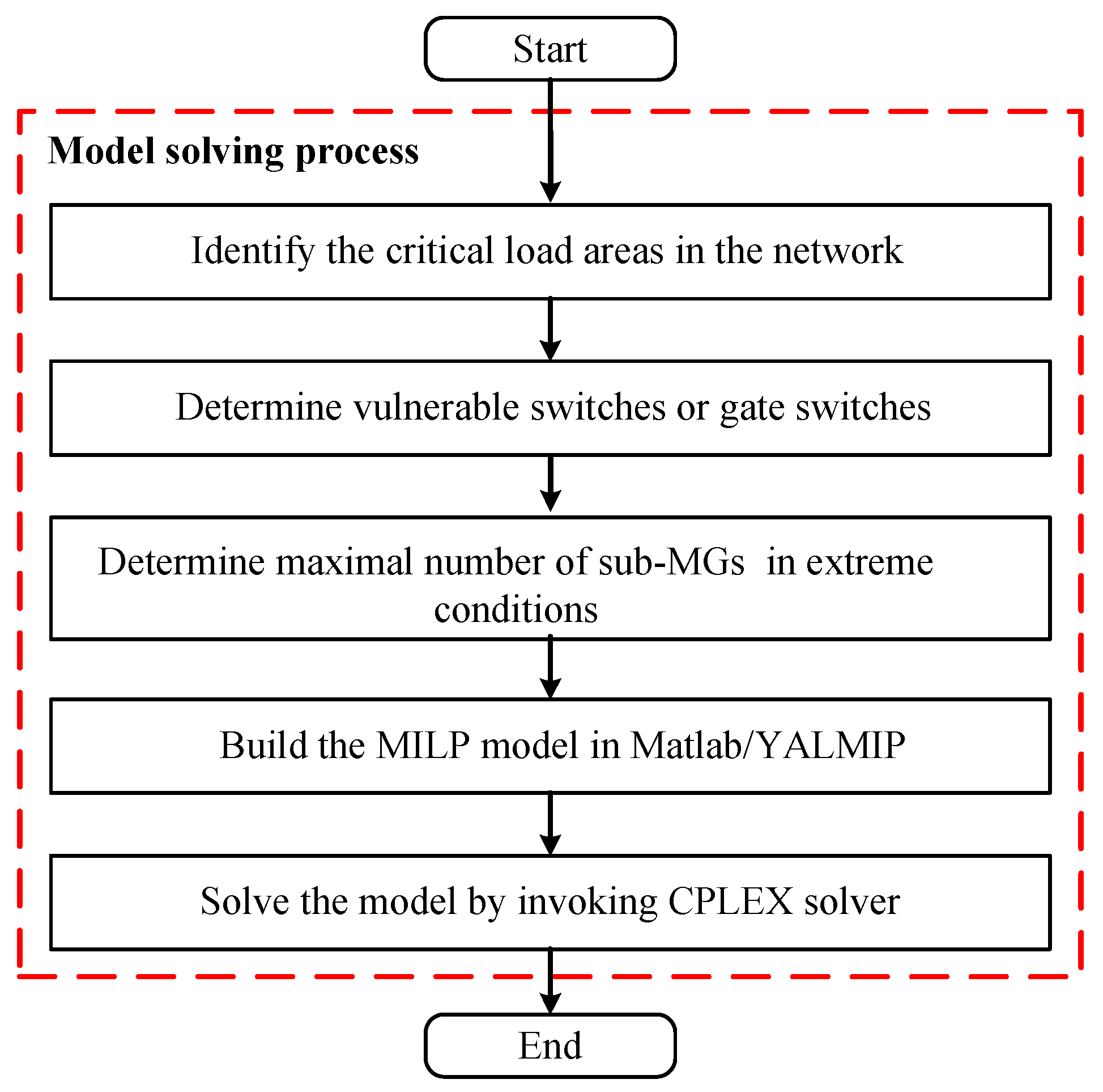
To sum up, the solving process of the proposed model is displayed in Figure 1.

Firstly, identify the critical load areas in the network. After that, determine the vulnerable switches or gate switches in the microgrid. If the vulnerable switches or gate switches passively or actively break due to external disturbances, it may lead to the formation of sub-MGs. Subsequently, determine the maximal number of sub-MGs which depends on local conditions. If the local area is in a good condition, the maximal number of sub-MGs can be set to 1 as an autonomous microgrid. However, if the local area easily suffers from extreme conditions such as hurricanes, the maximal number of sub-MGs can be more. Since then, the parameters are determined. Finally, the MILP model is built in Matlab/Yalmip and solved by invoking CPLEX solver.

4. Case Study

For purpose of validating the effectiveness of the established model and algorithm, the IEEE 33-bus distribution system [30] and IEEE 123-bus distribution system [31] are chosen as case studies to be researched. Using YALMIP in Matlab, the proposed model is programmed. After that, the solver CPLEX is invoked to solve the model in a desktop with Intel Pentium 2.2 GHz processor and 8 GB memory.

4.1. Case Study I: IEEE 33-Bus Distribution System

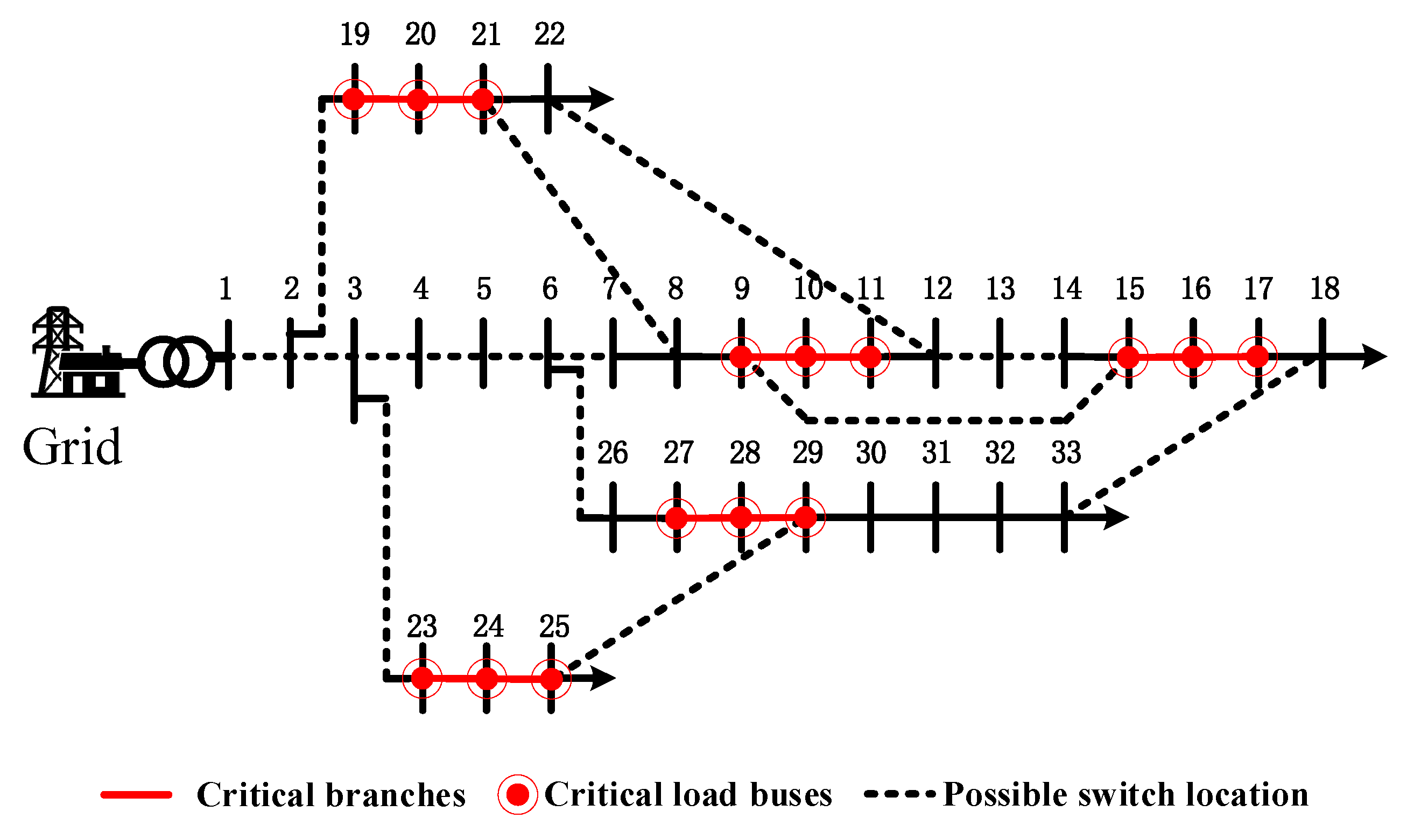
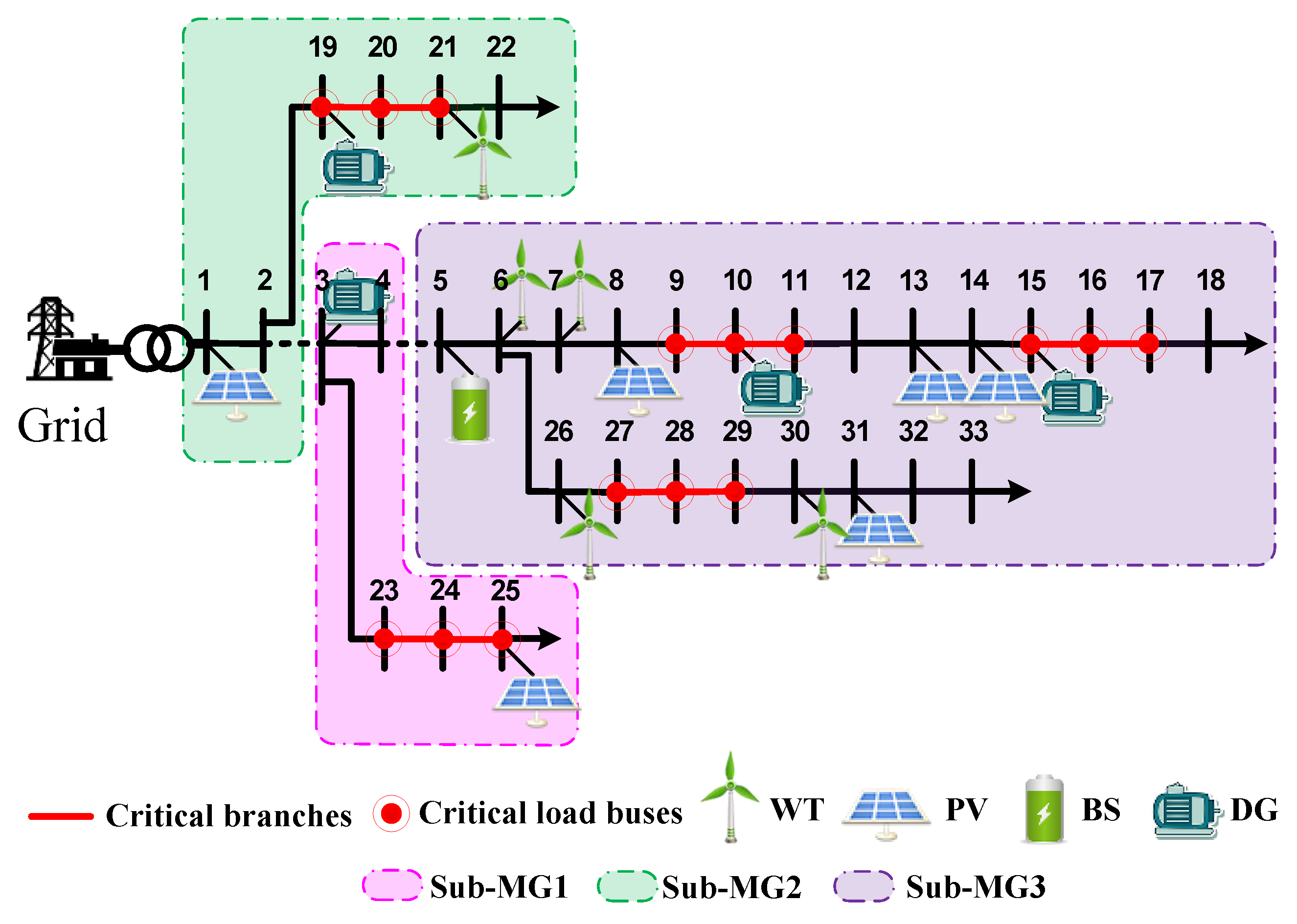
The configuration of the microgrid is given in Figure 2, the critical load buses and branches are identified with red color. The possible switches dividing the microgrid into sub-microgrids are marked with dash lines. The peak load in the microgrid is approximately 3 MW, and the critical load in the microgrid is approximately 1.5 MW. The alternative DERs are composed of 6 DGs, 5 WTs, 6 PVs, and 4 BSs. The DER parameters are given in

Table 1. Technical parameters of DERs.

Type	Rated Power (kW)	Investment ($/kW)	Lifespan (year)	Fuel Cost ($/kWh)	Number Limit
DG	400	300	10	0.16	6
WT	200	1200	20	0	5
PV	250	1600	20	0	6

and

Table 2. Technical parameters of BSs.

Type	Pmax (kW)	Emax (kWh)	Power Cost ($/kW)	Energy Cost ($/kWh)	Lifespan (Year)	Number Limit
BS	200	500	270	150	15	4

. The data used are mainly referred to [32,33,34]. Assuming that the charging and discharging efficiency of the BSs are both 0.9. The BSs are under half charge statue as the initial value. The electricity prices are given in

Table 3. Electricity prices

Time of Use	Off-Peak1 (23–07)	Off-Peak2 (07–10,15–18,21–23)	Peak1 (10–11,13–15,18–21)	Peak2 (11–13)
Electricity price ($/kWh)	0.057	0.126	0.198	0.216

. Note that the electricity prices are dynamic in reality [35,36,37]. However, since it is not the focus of this paper, a static time of use price is applied for simplicity. Assume the selling price is 0.8 times as many as the buying price. The typical weekday and weekend for each of the four seasons of the year are selected.

The effectiveness of the established model is tested by three cases. Sub-microgrid is substituted with “sub-MG” in the following analysis for simplicity.

Case 1: 1 sub-MG as a conventional autonomous microgrid is considered, |SM| = 1;

Case 2: 3 sub-MGs with predetermined area are considered, |SM| = 3;

Case 3: 3 sub-MGs without predetermined area are considered, |SM| = 3;

(1) Case 1

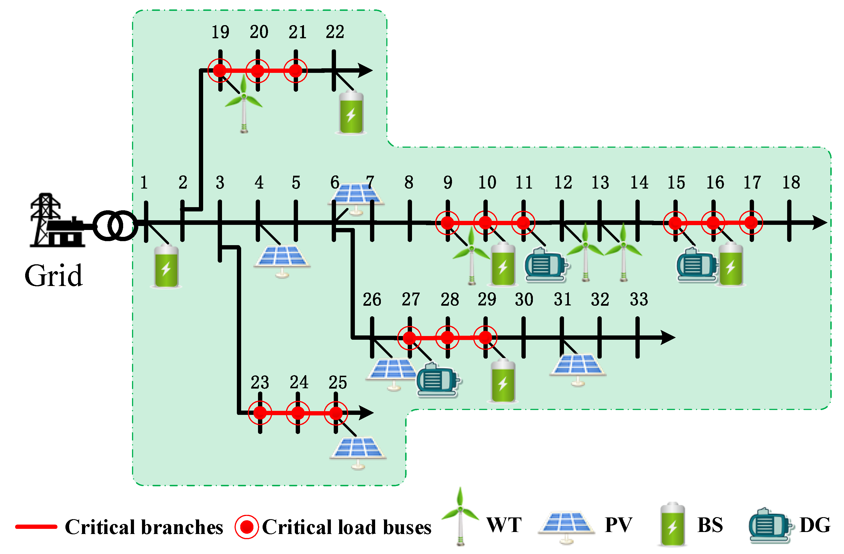
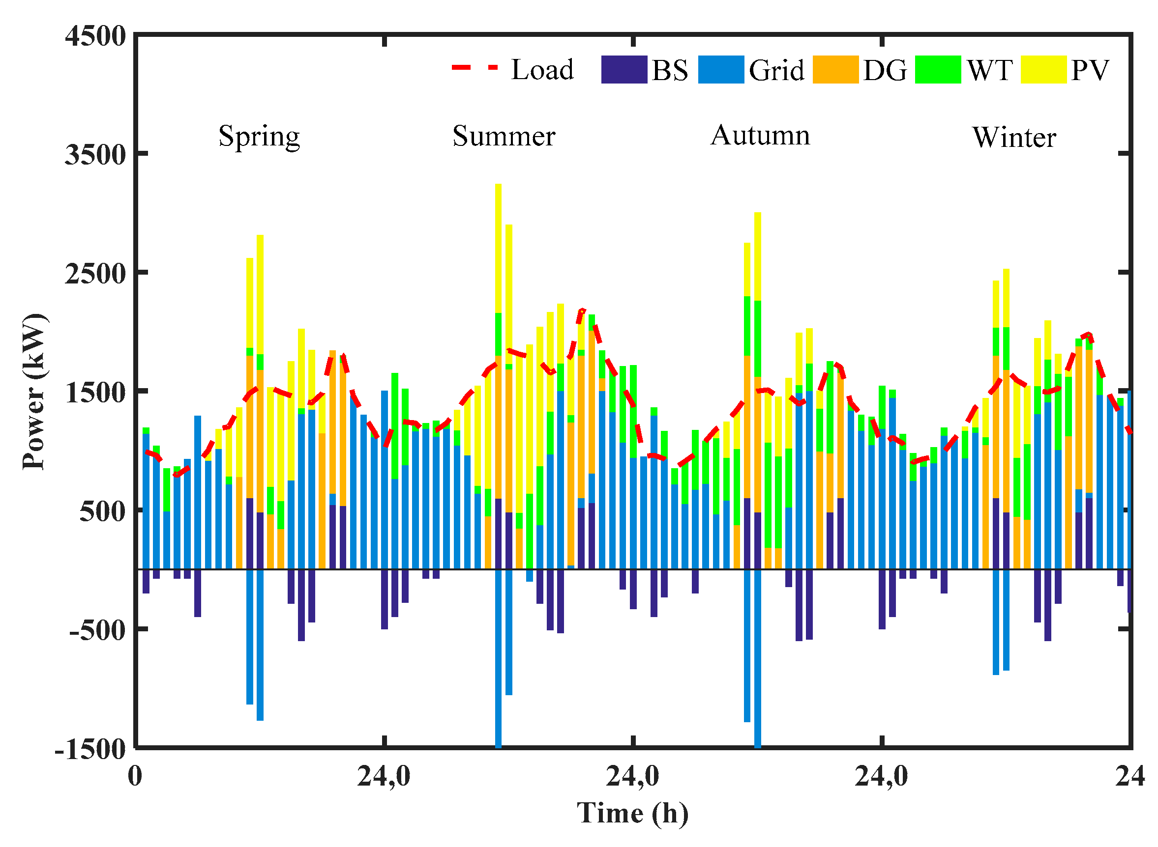
Firstly, 1 sub-MG is considered, and the distribution system is regarded as one microgrid. Namely, |SM| = 1. The conventional economic investment of DERs in interconnected mode and supply adequacy of critical loads in islanded mode are considered in this case. The construction of DERs in the microgrid are shown in Figure 3.

Table 4. Annual cost and generation of DERs in the microgrid.

DER	Investment Cost ($)	Operation Cost ($)	Generation Amount (MWh)	Average Cost ($/kWh)
DG1	1870	164,898	1022	0.180
DG2	1870	130,647	8100	0.184
DG3	1870	131,079	812	0.184
BS1	16,003	-	566	-
BS2	16,003	-	551	-
BS3	16,003	-	549	-
WT1-WT5	26,291	0	403	0.065
PV1-PV6	43,818	0	390	0.112

shows the annual cost and generation amount of DERs. The generation schedule of DERs in typical days in the year is shown in Figure 4.

As can be seen in Table 4, half of the candidate DGs are erected. It is worth noting that the generation of DGs is expensive from Table 4, while these DGs are selected to meet the requirements of load when the microgrid is in islanded mode in case of faults. Since DGs are expensive, their constructions are as less as possible provided the critical load is satisfied. Due to the relatively attractive price of renewable energy resources, all the candidate WTs and PVs are installed in the microgrid. In addition, WTs are more economical than PVs. The unit construction cost of WTs is fewer than that of PVs. Additionally, the wind resource is superior to the solar resource so that WTs will gain more profit. The BSs are also constructed. It is owing to that BSs can utilize the price difference of peak and valley electricity to reduce the cost. The detailed cost and generation amount of the DERs is recorded in Table 4. It is clear that the average cost of DGs is higher than that of other DERs and the electricity price. One point that should be noted is that DGs do not generate power most of the time. They generate power only if the electricity price is high at peak time. The table also shows that the average cost of WTs and PVs is greatly lower than that of other DERs.

The generation schedule result of DERs in the microgrid with typical days of the year is shown in Figure 4. DGs run to meet the load because of the considerably high load level. Since the generation of WTs and PVs is lowly consumed, WTs and PVs are efficiently used to generate power. The great mass of the power is from the utility grid because of the restricted capacity of DERs. During the day, the BSs utilize the price difference of peak and valley electricity to earn profit. The BSs charge during off-peak1/off-peak2 h and discharge during peak1/peak2 h. It demonstrates the economy of the schedule and verifies the effectiveness of the developed model.

(2) Case 2

In Case 2, |SM| = 3, and 3 sub-MGs with predetermined area are considered. In this case, the predetermined area of the sub-MGs and the obtained optimal placement of DERs are shown in Figure 5.

In each sub-MG, the critical load should be fulfilled without load loss. In sub-MG1, there are one DG and one PV to supply the critical load. In sub-MG2, one DG, one PV and one WT are installed to satisfy the critical load. In sub-MG3, many DERs are distributed there to satisfy three critical load areas. Note that each sub-MG is equipped with at least one DG. This is because the DG has a larger capacity than the other DERs, and it is able to dominate the frequency and voltage in the sub-MG. Therefore, to guarantee the supply adequacy of critical loads in the sub-MG, at least one DG is installed in each sub-MG. The annual cost in this case is $1,487,847, which is more than that in Case 1. This is because more critical loads need to be supplied separately, the arrangement of DERs in one microgrid may fail to satisfy the critical loads in the sub-MGs. Therefore, more DERs are installed to guarantee the supply adequacy of sub-MGs, and more investment cost is needed.

(3) Case 3

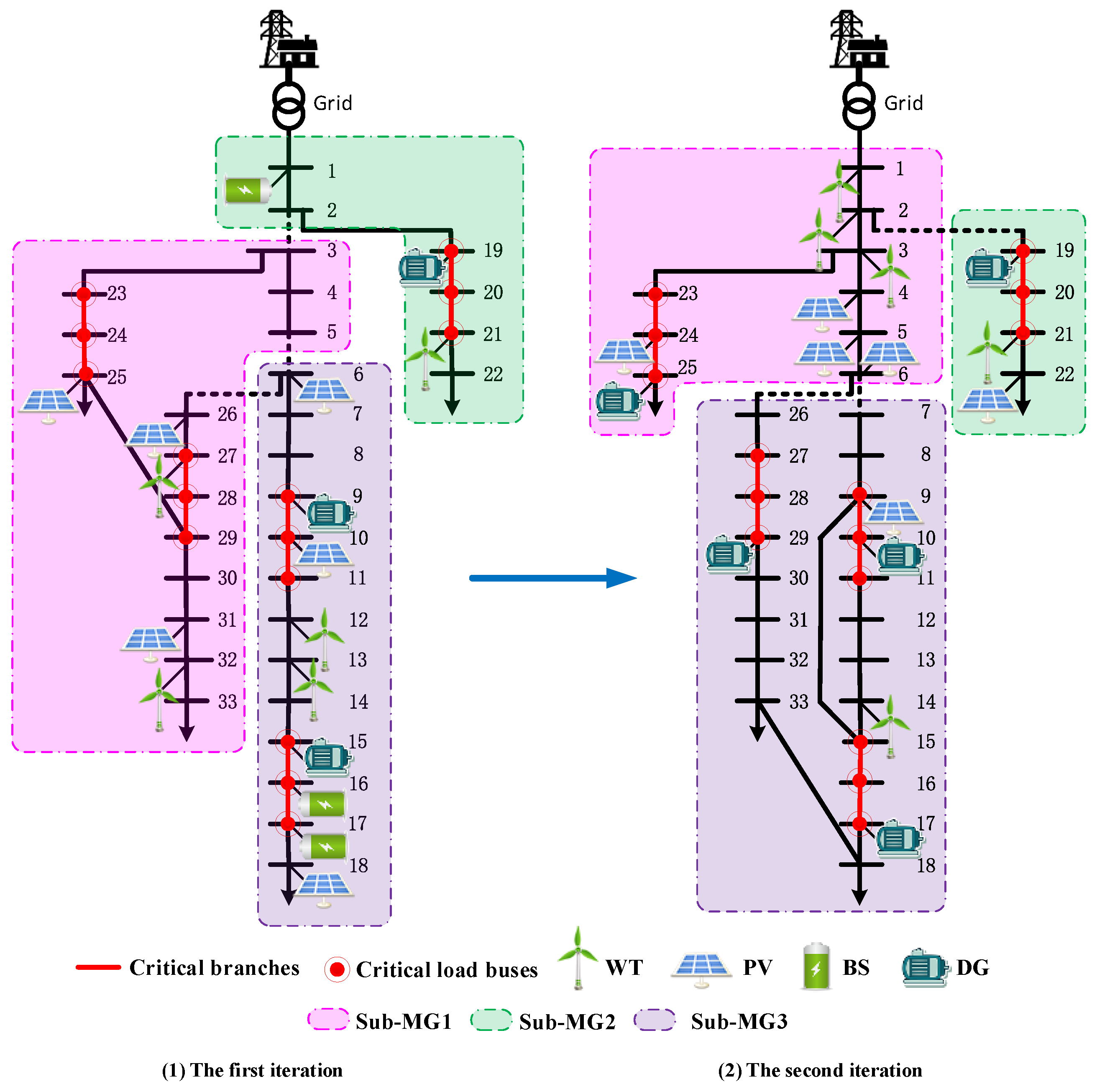
In Case 3, the uncertain formation of sub-MGs is considered. The formation of sub-MGs and placement of DERs during the iterations in Case 3 are shown in Figure 6.

The area of sub-MGs is not predetermined in this case. The procedure ends after two iterations. The optimization always identifies the worst formation of sub-MGs. This is easy to be observed in Figure 6. The area of sub-MGs and switch locations that divide the network into sub-MGs are completely different from those in Case 2. Similar to Case 2, DGs are mostly placed around the critical load area. Therefore, critical loads can always be supplied. Note that the annual cost in Case 3 is more than that in Case 2, and the placement of DERs in the microgrid is different. However, the placement of DERs in Case 3 is more robust than that in Case 2. It is because it can supply critical loads under the worst formation of sub-MGs.

More cases are conducted when the number of sub-MGs (|SM|) increases from 1 to 5. The number and type of DERs are listed in

Table 5. Number of installed DERs with the increase of sub-MGs.

|SM|	DG	BS	WT	PV
1	3	3	5	6
2	4	1	5	6
3	5	0	5	6
4	5	0	5	6
5	5	0	5	6

. From Table 5, with the increase of sub-MGs, the number of DGs increases from 3 to 5, while the number of BSs decreases from 3 to 0. As more sub-MGs are formed, more DGs are needed to maintain the power supply of critical load areas. It also brings an increase in annual cost. The capacity of a DG is twice larger than that of a BS. Increasing one DG is equivalent to reducing one or two BSs from the perspective of power supply. Therefore, the number of BSs decreases with the increase of the number of DGs. Since the generation cost of WTs and PVs is considerably low, all the WTs and PVs are installed in those cases.

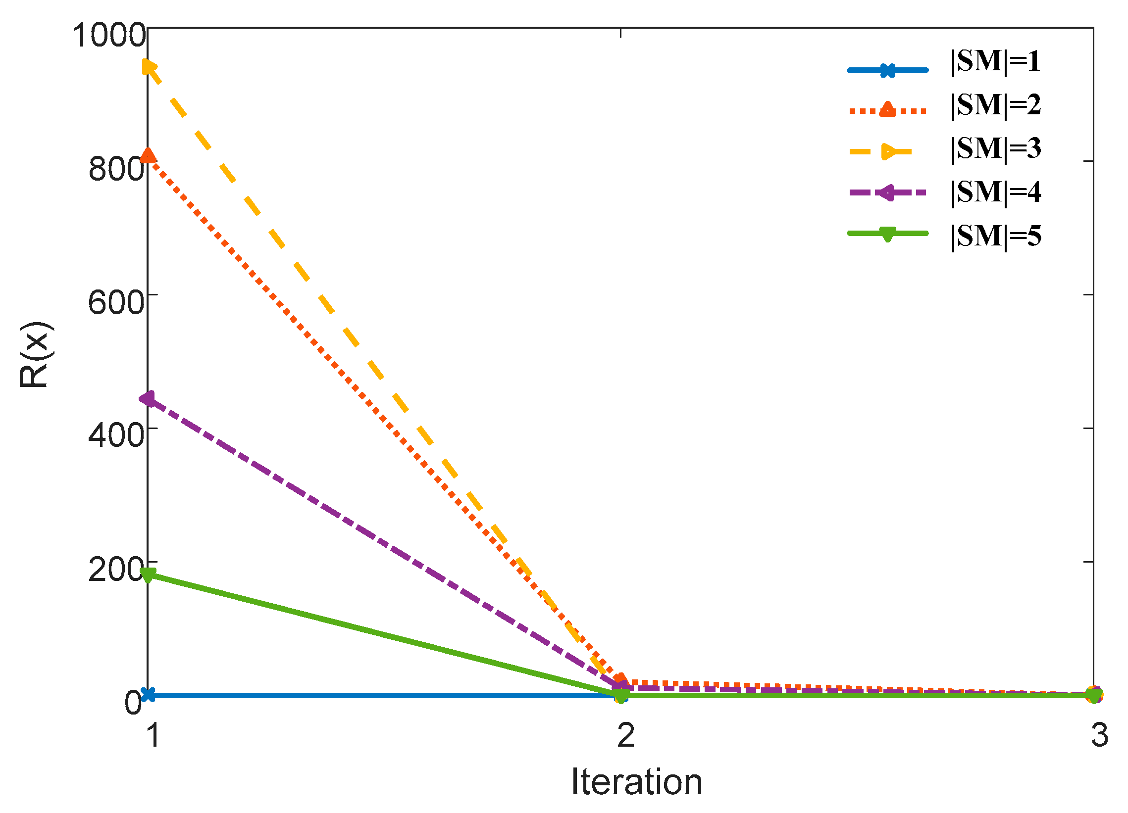
Figure 7 gives the value of the feasibility checking function during the iterations in cases when |SM| increases from 1 to 5. As can been seen, the value in all cases decreases to zero after at most 3 iterations. This can be explained by the fact that more DERs may be added in the microgrid after each iteration. The unserved loads will definitely drop to zero at last with the increase of power sources during the iterations.

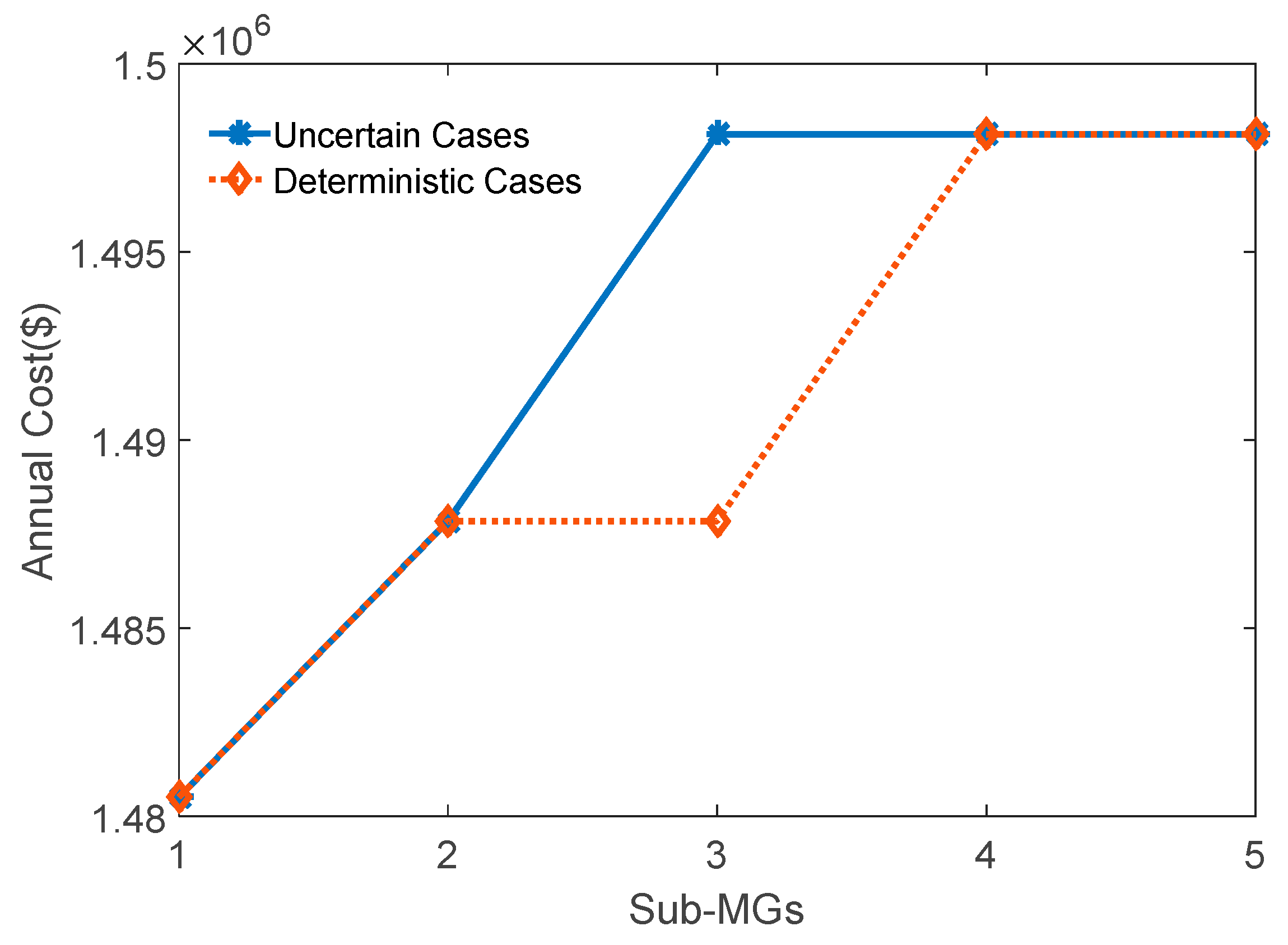
Figure 8 gives the annual cost in cases when |SM| increases from 1 to 5. The results under deterministic and uncertain formation of sub-MGs are compared.

In the cases under uncertain formation of sub-MGs, the annual cost increases from $1,480,508 to $1,498,123 with the increase of sub-MGs. Note that the cost remains unchanged when the number of sub-MGs increases to 3. This is because the power sources are enough to support the power supply of critical load area regardless of the partition of sub-MGs. However, the placement strategy of DERs in the case |SM| = 5 is more robust than that in the cases |SM| = 4 or |SM| = 3. It is because any realization of 5 sub-MGs can guarantee the supply adequacy of the critical loads. In the cases under deterministic formation of sub-MGs, the annual cost also increases with the increase of sub-MGs. However, in most of the cases, the annual cost is the same as that under uncertain formation of sub-MGs. As can be seen, there is a difference only when the number of sub-MGs is 3. Therefore, the robust placement of DERs will not necessarily cause a higher investment.

The computational time of the proposed method in the studied case is specified in

Table 6. Computational time of Case Study I.

|SM|	1	2	3	4	5
Iteration	1	3	2	3	2
Computational Time (s)	3	8	3	7	4

.

As can be seen in Table 6, the computational time in all the cases is only several seconds. This is mainly because the optimization problem is a small-scale MILP problem, which could be easily solved by the commercial solver. In addition, the optimization problem takes only a few iterations in each case.

4.2. Case Study II: IEEE 123-Bus Distribution System

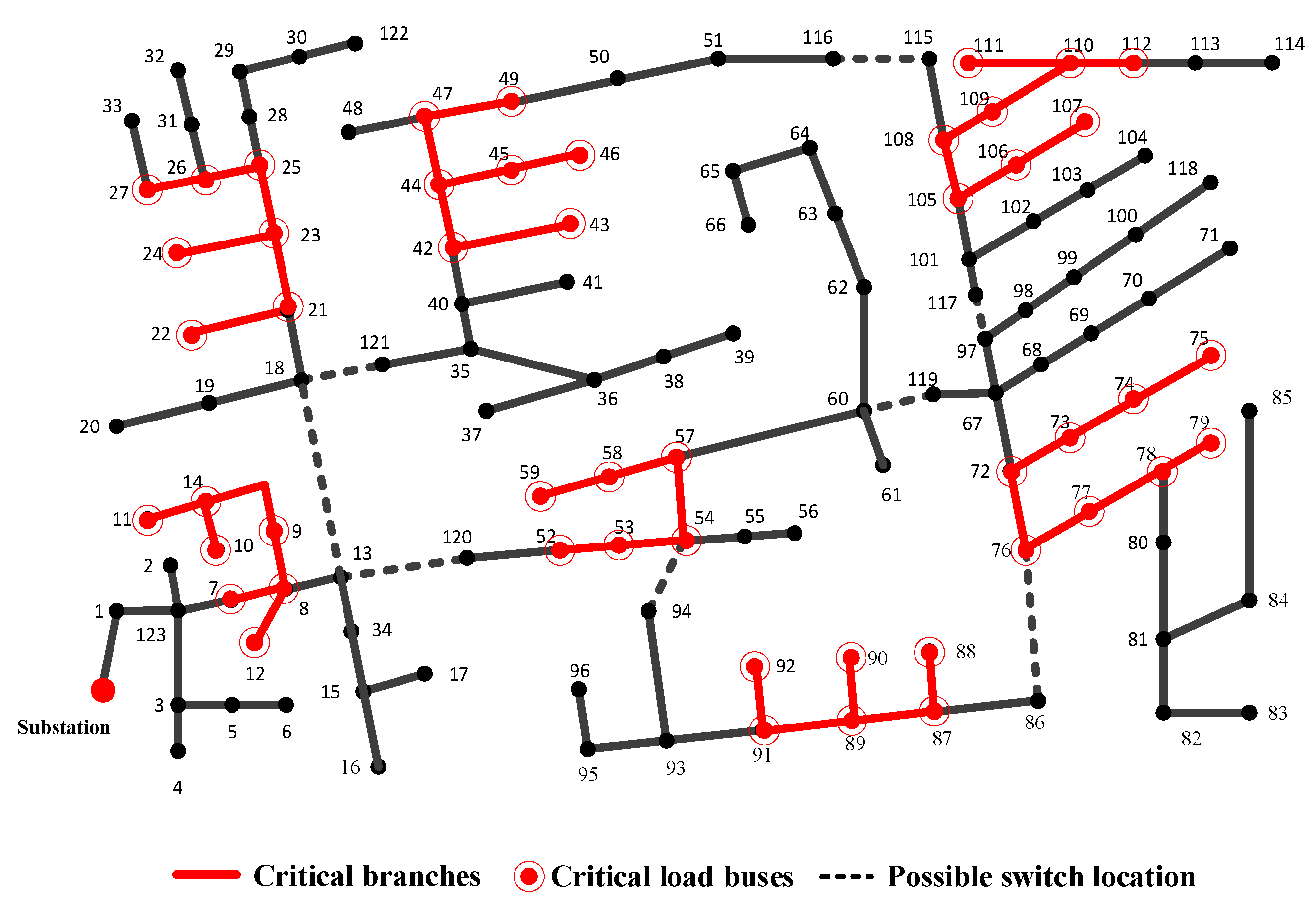
A microgrid case based on IEEE 123-bus distribution system is also studied. The configuration of the distribution system is given in Figure 9. The parameters of candidate DERs are shown in

Table 7. Technical parameters of DERs.

Type	Rated Power (kW)	Investment ($/kW)	Lifespan (Year)	Fuel Cost ($/kWh)	Number Limit
DG	200	300	10	0.16	10
WT	150	1200	20	0	8
PV	250	1600	20	0	6

and

Table 8. Technical parameters of BSs.

Type	Pmax (kW)	Emax (kWh)	Power Cost ($/kW)	Energy Cost ($/kWh)	Lifespan (Year)	Number Limit
BS	200	500	270	150	15	6

. The other parameters such as electricity price and load level are the same as those in Case Study I.

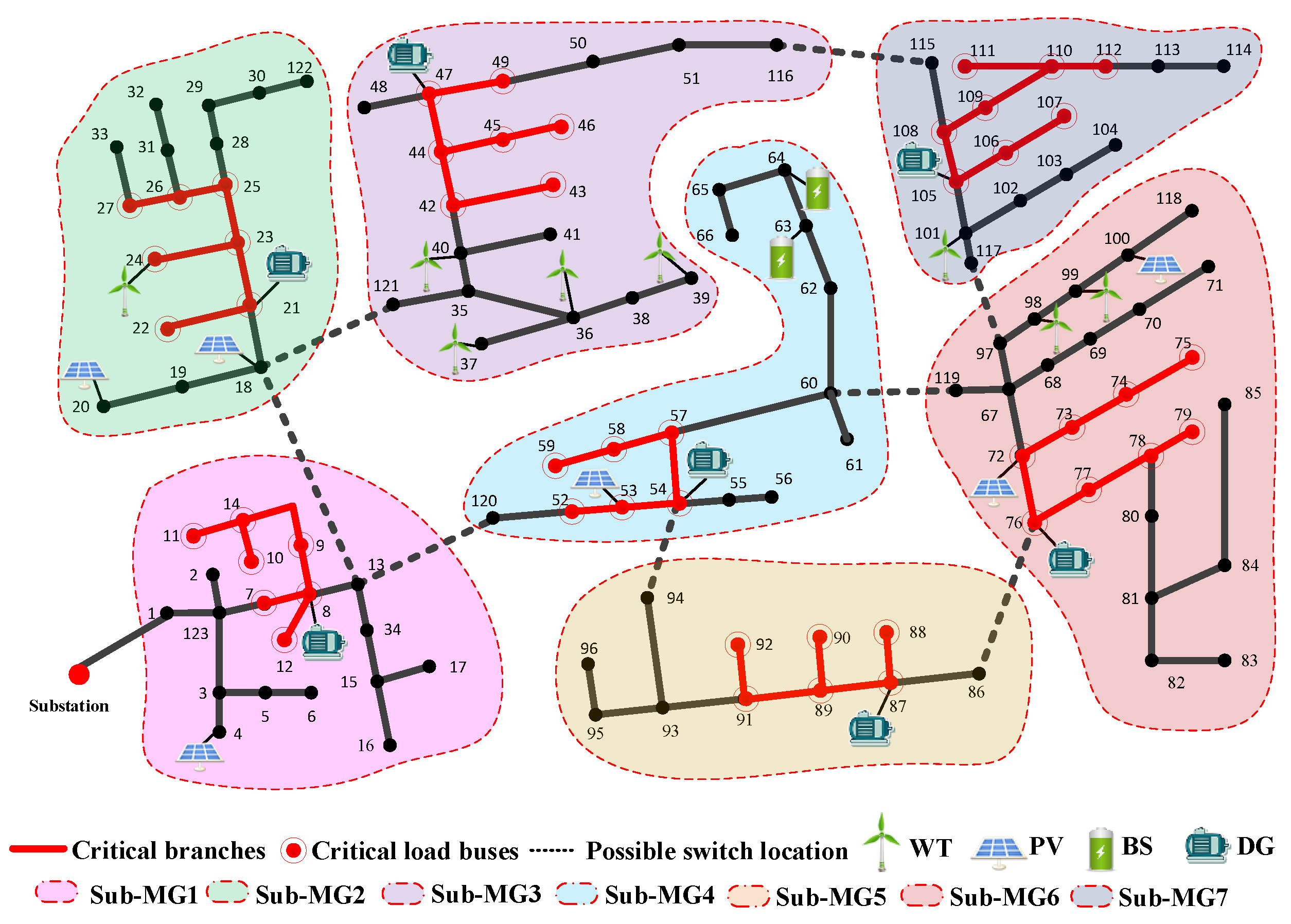
The cases when |SM| increases from 1 to 7 are conducted. Figure 10 shows the construction of DERs in the microgrid when 7 sub-MGs are formed. In this situation, the result is the same as that in deterministic case because the microgrid can be partitioned into at most 7 sub-MGs. As can be seen, each sub-MG has at least one DER. Some sub-MGs have more DERs because there are more critical loads there.

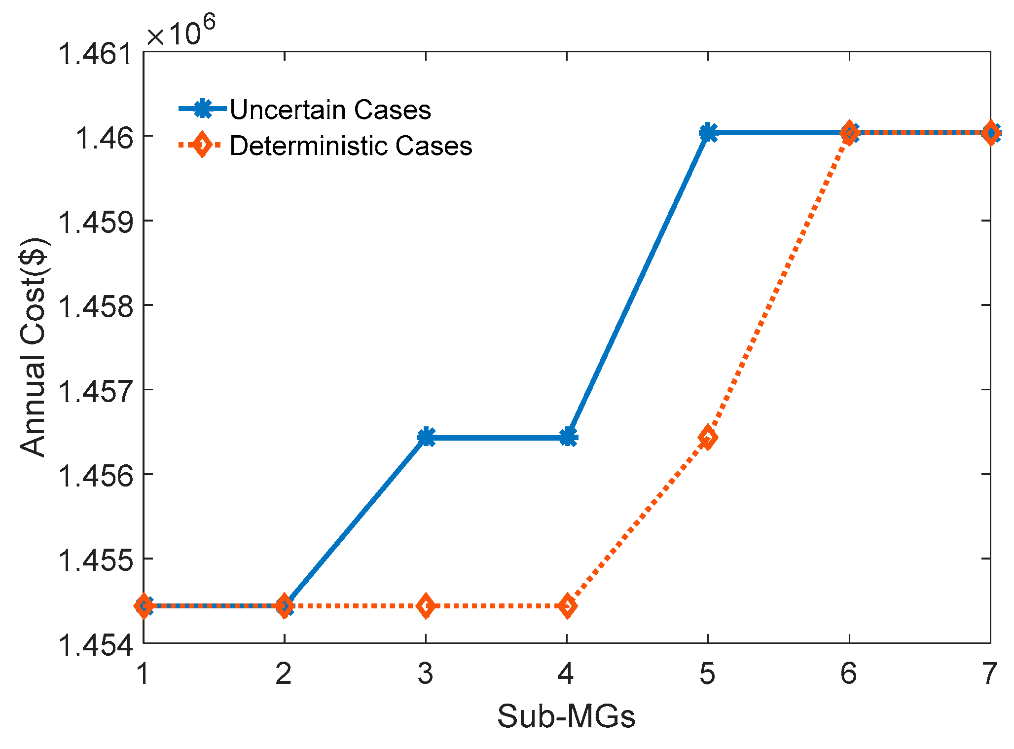
The annual costs under uncertain and deterministic formation of sub-MGs are compared too. As can be seen in Figure 11, the annual cost is the same as that under deterministic formation of sub-MGs in four cases. It further indicates that the robust placement of DERs will not necessarily cause a higher investment. The detailed arrangement of DERs under the uncertain formation of sub-MGs is given in

Table 9. Number of installed DERs with the increase of sub-MGs.

|SM|	DG	BS	WT	PV
1	5	4	8	6
2	5	4	8	6
3	6	3	8	6
4	6	3	8	6
5	7	2	8	6
6	7	2	8	6
7	7	2	8	6

.

The computational time of the proposed method in Case Study II is specified in

Table 10. Computational time of Case Study II.

|SM|	1	2	3	4	5	6	7
Iteration	1	6	5	3	3	2	2
Computational Time (s)	6	67	154	66	28	16	16

.

As can be seen in Table 10, the computational time in all the cases is within several minutes, which is acceptable for a planning problem. In addition, more iterations generally mean more computational time.

As analyzed above, the critical loads can be supplied in several sub-MGs. The proposed model can guarantee the supply adequacy of critical loads regardless of the formation of sub-MGs. Most strategies cost no more than those in deterministic cases. However, the strategies are more robust. It should be noted that the robustness of the model can be controlled by predetermining the switch states. If the states of switches are all predetermined, the model becomes a deterministic one.

5. Conclusions

In this paper, a microgrid planning model considering the supply adequacy of critical loads under uncertain formation of sub-microgrids is established to optimally place the DERs. To make the microgrid capable of supplying the critical loads within the sub-microgrids in case of multiple power outages, the supply adequacy constraints are strengthened in the planning model. The problem is finally formulated as a robust optimization problem and solved by the C&CG method. Different from conventional microgrid planning models, which only consider the interconnected or islanded mode, the proposed model is able to consider more serious situation that the microgrid suffers from multiple faults and is split into several sub-MGs. In addition, compared to deterministic method, the proposed method is more robust as critical load loss is intolerable. Finally, the case studies indicate that the investment cost would not necessarily be more than that in the deterministic case. Specifically, the investment costs are the same when the number of sub-MGs is within two. Since most of simultaneous faults are less than threefold, the proposed model is applicable as it is more robust with the same cost.

References

- Di Somma, M.; Graditi, G.; Siano, P. Optimal Bidding Strategy for a DER Aggregator in the Day-Ahead Market in the Presence of Demand Flexibility. IEEE Trans. Ind. Electron. 2019, 66, 1509–1519. [Google Scholar] [CrossRef]
- Di Somma, M.; Yan, B.; Bianco, N.; Luh, P.B.; Graditi, G.; Mongibello, L.; Naso, V. Multi-objective operation optimization of a Distributed Energy System for a large-scale utility customer. Appl. Therm. Eng. 2016, 101, 752–761. [Google Scholar] [CrossRef]
- Stevanoni, C.Z.; Grève, D.; Vallée, F.; Deblecker, O. Long-Term Planning of Connected Industrial Microgrids: A Game Theoretical Approach Including Daily Peer-to-Microgrid Exchanges. IEEE Trans. Smart Grid 2019, 10, 2245–2256. [Google Scholar] [CrossRef]
- Zhang, J.; Li, K.J.; Wang, M.; Lee, W.J.; Gao, H. A Bi-Level Program for the Planning of an Islanded Microgrid Including CAES. In Proceedings of the 2015 IEEE Industry Applications Society Annual Meeting, Addison, TX, USA, 18–22 October 2015; pp. 1–8. [Google Scholar]
- Khodaei, A.; Bahramirad, S.; Shahidehpour, M. Microgrid Planning Under Uncertainty. IEEE Trans. Power Syst. 2015, 30, 1–9. [Google Scholar] [CrossRef]
- Khodaei, A. Provisional microgrid planning. IEEE Trans. Smart Grid 2017, 8, 1096–1104. [Google Scholar] [CrossRef]
- Wang, Z.; Chen, B.; Wang, J.; Kim, J.; Begovic, M.M. Robust Optimization Based Optimal DG Placement in Microgrids. IEEE Trans. Smart Grid 2014, 5, 2173–2182. [Google Scholar] [CrossRef]
- Guo, L.; Hong, B.; Jiao, B.; Liu, W.; Wang, C. Multi-objective stochastic optimal planning method for stand-alone microgrid system. IET Gener. Transm. Distrib. 2014, 8, 1263–1273. [Google Scholar] [CrossRef]
- Graditi, G.; Di Silvestre, M.L.; Sanseverino, E.R. A Generalized Framework for Optimal Sizing of Distributed Energy Resources in Micro-Grids Using an Indicator-Based Swarm Approach. IEEE Trans. Ind. Inform. 2014, 10, 152–162. [Google Scholar]
- Ailvia, J.F.; Carlos, C.G.; Ricardo, M.P.; Juan, C.F.; Javier, D.S.; Antonio, P.F.; Sancho, S.S. Optimal Microgrid Topology Design and Siting of Distributed Generation Sources Using a Multi-Objective Substrate Layer Coral Reefs Optimization Algorithm. Suntainability 2019, 11, 1–21. [Google Scholar]
- Liu, Z.; Yang, J.; Zhang, Y.; Ji, T.; Zhou, J.; Cai, Z. Multi-Objective Coordinated Planning of Active-Reactive Power Resources for Decentralized Droop-Controlled Islanded Microgrids Based on Probabilistic Load Flow. IEEE Access 2018, 6, 40267–40280. [Google Scholar] [CrossRef]
- Basu, A.K.; Chowdhury, S.; Chowdhury, S.P. Impact of Strategic Deployment of CHP-Based DERs on Microgrid Reliability. IEEE Trans. Power Deliv. 2010, 25, 1697–1705. [Google Scholar] [CrossRef]
- Hakimi, S.M.; Moghaddas-Tafreshi, S.M. Optimal Planning of a Smart Microgrid Including Demand Response and Intermittent Renewable Energy Resources. IEEE Trans. Smart Grid 2014, 5, 2889–2900. [Google Scholar] [CrossRef]
- Moradi, M.H.; Eskandari, M.; Hosseinian, S.M. Operational Strategy Optimization in an Optimal Sized Smart Microgrid. IEEE Trans. Smart Grid 2015, 6, 1087–1095. [Google Scholar] [CrossRef]
- Mitra, J.; Vallem, M.R.; Singh, C. Optimal Deployment of Distributed Generation Using a Reliability Criterion. IEEE Trans. Ind. Appl. 2016, 52, 1. [Google Scholar] [CrossRef]
- Wang, H.; Huang, J. Cooperative Planning of Renewable Generations for Interconnected Microgrids. IEEE Trans. Smart Grid 2016, 7, 1. [Google Scholar] [CrossRef]
- Che, L.; Zhang, X.P.; Shahidehpour, M.; AlAbdulwahab, A.; Abusorrah, A. Optimal Interconnection Planning of Community Microgrids with Renewable Energy Sources. IEEE Trans. Smart Grid 2017, 8, 1. [Google Scholar] [CrossRef]
- Ju, C.; Yao, S.; Wang, P. Resilient Post-Disdter System Reconfiguration for Multiple Energy Service Restoration. In Proceedings of the 2017 IEEE Conference on Energy Internet and Energy System Integration (EI2), Beijing, China 26–28 November 2017; pp. 1–6. [Google Scholar]
- Wang, Z.; Wang, J.; Chen, C. A Three-Phase Microgrid Restoration Model Considering Unbalanced Operation of Distributed Generatio. IEEE Trans. Smart Grid 2018, 9, 3594–3604. [Google Scholar] [CrossRef]
- Manshadi, S.D.; Khodayar, M.E. Resilient Operation of Multiple Energy Carrier Microgrids. IEEE Trans. Smart Grid 2015, 6, 1. [Google Scholar] [CrossRef]
- Manshadi, S.D.; Khodayar, E.M. Expansion of Autonomous Microgrids in Active Distribution Networks. IEEE Trans. Smart Grid 2016, PP, 1. [Google Scholar] [CrossRef]
- Arefifar, S.A.; Mohamed, Y.A.R.I.; El-Fouly, T.H.M. Supply-Adequacy-Based Optimal Construction of Microgrids in Smart Distribution Systems. IEEE Trans. Smart Grid 2012, 3, 1491–1502. [Google Scholar] [CrossRef]
- Chen, C.; Wang, J.; Qiu, F.; Zhao, D. Resilient Distribution System by Microgrids Formation after Natural Disasters. IEEE Trans. Smart Grid 2015, 7, 958–966. [Google Scholar] [CrossRef]
- Nassar, M. Microgrid Enabling Towards the Implementation of Smart Grids. PhD Thesis, University of Waterloo, Waterloo, ON, Canada, 2017. [Google Scholar]
- Liu, Z.; Wang, X.; Zhuo, R.; Cai, X. Flexible network planning of autonomy microgrid. IET Renew. Power Gener. 2018, 12, 1931–1940. [Google Scholar] [CrossRef]
- Balakrishnan, R.; Ranganathan, K. A Textbook of Graph Theory. Math. Gaz. 2000, 84. [Google Scholar]
- Ding, T.; Lin, Y.; Li, G.; Bie, Z. A New Model for Resilient Distribution Systems by Microgrids Formation. IEEE Trans. Power Syst. 2017, 32, 4145–4147. [Google Scholar] [CrossRef]
- McCormick, G.P. Computability of global solutions to factorable nonconvex programs-1. convex underestimating problems. Math. Program. 1976, 10, 147–175. [Google Scholar] [CrossRef]
- Zeng, B.; Zhao, L. Solving two-stage robust optimization problems using a column-and-constraint generation method. Oper. Res. Lett. 2013, 41, 457–461. [Google Scholar] [CrossRef]
- Baran, M.E.; Wu, F.F. Network reconfiguration in distribution systems for loss reduction and load balancing. IEEE Trans. Power Deliv. 1992, 4, 1401–1407. [Google Scholar] [CrossRef]
- Kersting, W.H. Radial Distribution Test Feeders. In Proceedings of the 2001 IEEE Power Engineering Society Winter Meeting. Conference Proceedings (Cat. No. 01CH37194), Columbus, OH, USA, 28 January–1 February 2001; pp. 908–912. [Google Scholar]
- Zou, K.; Agalgaonkar, A.P.; Muttaqi, K.M.; Perera, S. Distribution System Planning with Incorporating DG Reactive Capability and System Uncertainties. IEEE Trans. Sustain. Energy 2012, 3, 112–123. [Google Scholar] [CrossRef]
- Zhang, J.; Cheng, H.; Wang, C. Technical and economic impacts of active management on distribution network. Int. J. Electr. Power Energy Syst. 2009, 31, 130–138. [Google Scholar] [CrossRef]
- Cao, X.; Wang, J.; Zeng, B. A Chance Constrained Information-Gap Decision Model for Multi-Period Microgrid Planning. IEEE Trans. Power Syst. 2018, 33, 2684–2695. [Google Scholar] [CrossRef]
- Parhizi, S.; Khodaei, A.; Shahidehpour, M. Market-based vs. Price-based Microgrid Optimal Scheduling. IEEE Trans. Smart Grid 2016, 9, 615–623. [Google Scholar] [CrossRef]
- Majzoobi, A.; Khodaei, A. Application of Microgrids in Supporting Distribution Grid Flexibility. IEEE Trans. Power Syst. 2016, 32, 3660–3669. [Google Scholar] [CrossRef] [Green Version]
- Manshadi, S.D.; Khodayar, M. A Hierarchical Electricity Market Structure for the Smart Grid Paradigm. In Proceedings of the 2016 IEEE Power and Energy Society General Meeting (PESGM), Boston, MA, USA, 17–21 July 2016; p. 7. [Google Scholar]