A Multivariate Geomorphometric Approach to Prioritize Erosion-Prone Watersheds

 ,
,  ,
,
Abstract
:1. Introduction
2. Materials and Methods
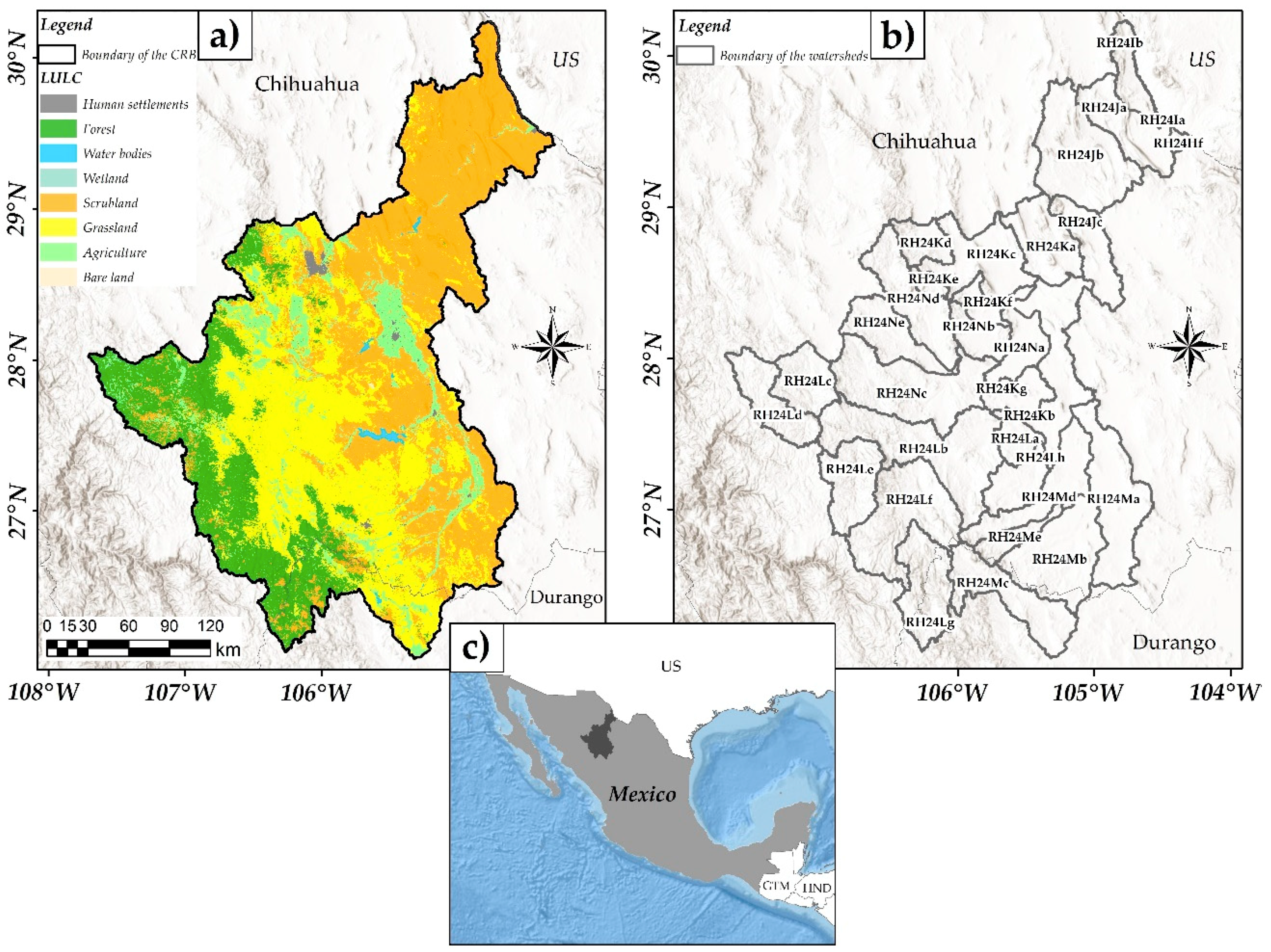
2.1. Study Area
2.2. Data
2.3. Watershed’s Description and Classification
2.4. Comparison of the Classification Methods
3. Results
3.1. Characterization of Conchos River Basin Watersheds
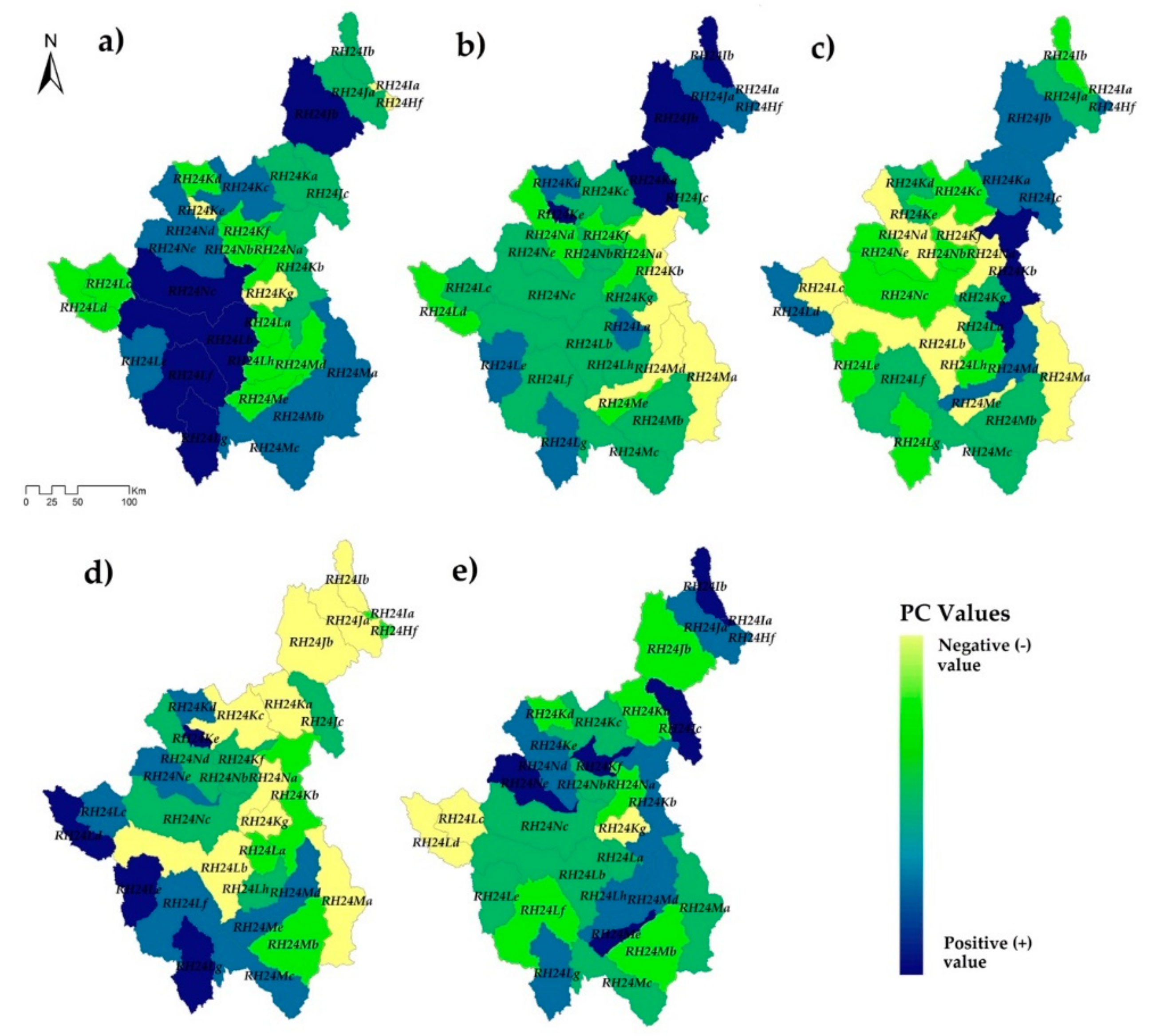
3.2. Correlations and Principal Component Analyses
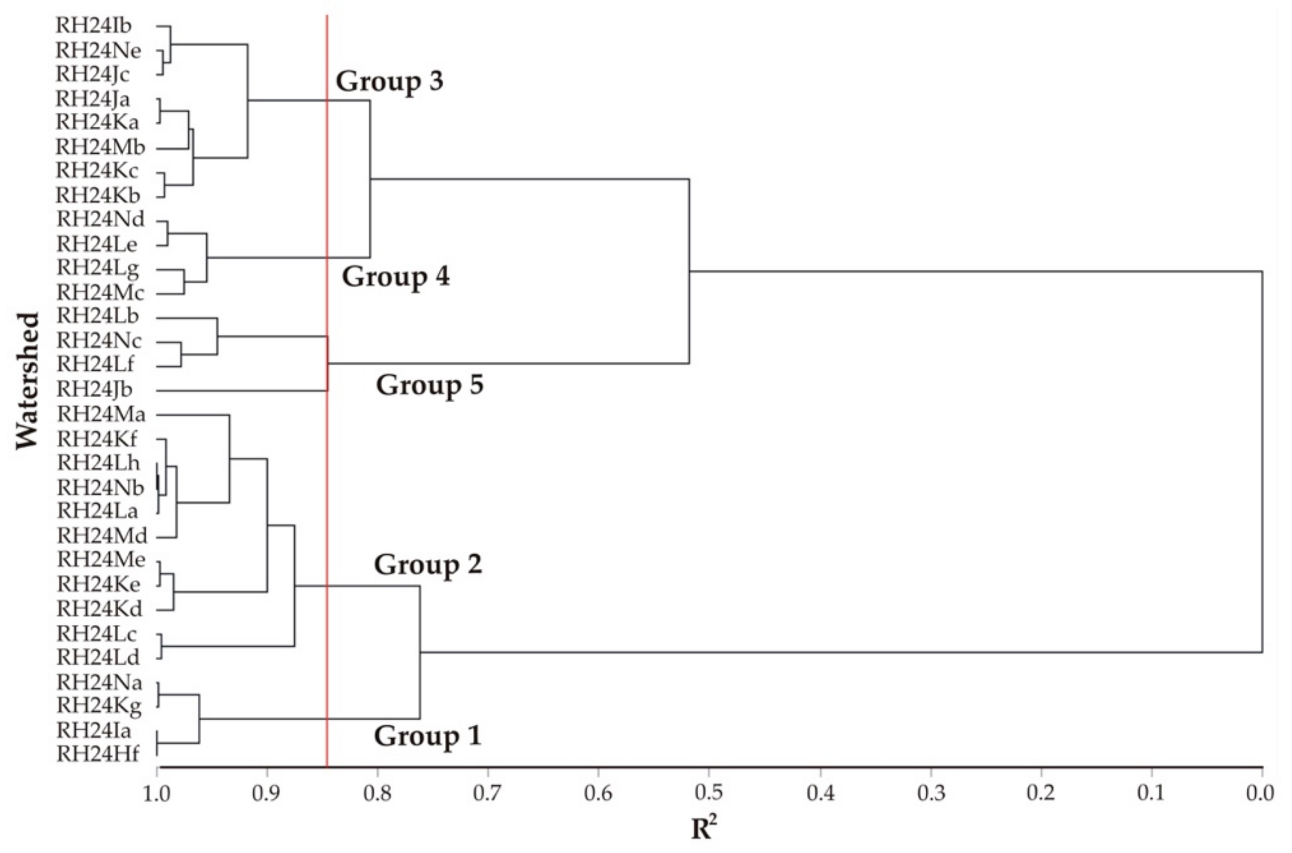
3.3. Watershed’s Classification Based on Group Analysis
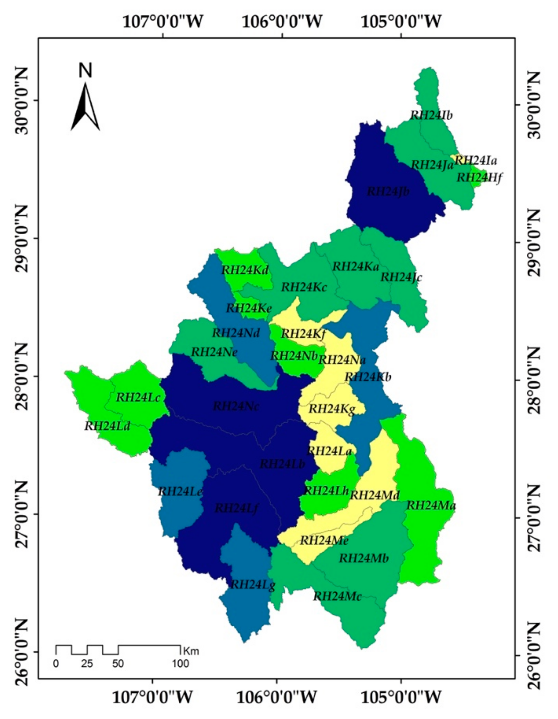
3.4. Watershed’s Classification Based on the Compound Parameter (Cp)
3.5. Comparison of the Classification Methods
4. Discussion
5. Conclusions
Author Contributions
Funding
Acknowledgments
Conflicts of Interest
Appendix A

| Wid | A | P | Lb2 | Lc | Li | Lu | Nu | No1 | Hmin | Hmax | Hmed | Cc | Re | Rf | Ia | J | tgα |
|---|---|---|---|---|---|---|---|---|---|---|---|---|---|---|---|---|---|
| RH24Hf | 183.19 | 71.99 | 12.18 | 12.66 | 123.87 | 505.43 | 649 | 336 | 940 | 1100 | 780 | 3.00 | 1.25 | 14.47 | 0.87 | 6.76 | 0.19 |
| RH24Ia | 78.62 | 50.60 | 24.19 | 11.17 | 69.21 | 189.88 | 252 | 111 | 920 | 1040 | 800 | 3.22 | 0.41 | 7.04 | 1.59 | 8.80 | 0.09 |
| RH24Ib | 1209.37 | 259.75 | 140.20 | 34.15 | 2261.86 | 3915.19 | 5039 | 2367 | 1470 | 2140 | 800 | 4.21 | 0.28 | 35.41 | 0.96 | 18.70 | 0.82 |
| RH24Ja | 2344.14 | 297.44 | 132.14 | 61.84 | 3197.22 | 6430.37 | 7716 | 3854 | 1470 | 2140 | 800 | 3.47 | 0.41 | 37.91 | 1.63 | 13.64 | 1.59 |
| RH24Jb | 4527.91 | 373.79 | 121.30 | 56.88 | 5415.42 | 14,899.51 | 28,074 | 13,371 | 1580 | 2260 | 900 | 3.13 | 0.63 | 79.60 | 0.71 | 11.96 | 2.87 |
| RH24Jc | 1880.25 | 290.99 | 40.60 | 82.93 | 1877.94 | 5304.81 | 8784 | 4197 | 1610 | 2240 | 980 | 3.79 | 1.21 | 22.67 | 3.66 | 9.99 | 1.17 |
| RH24Ka | 2345.09 | 283.55 | 104.99 | 45.81 | 3530.78 | 6993.14 | 8771 | 4431 | 1620 | 2240 | 1000 | 3.30 | 0.52 | 51.19 | 0.89 | 15.06 | 1.45 |
| RH24Kb | 3447.12 | 546.62 | 5.47 | 106.05 | 2200.40 | 7188.10 | 10,601 | 5123 | 1645 | 2210 | 1080 | 5.25 | 12.12 | 32.51 | 3.26 | 6.38 | 2.10 |
| RH24Kc | 2928.21 | 433.41 | 141.09 | 83.92 | 3015.00 | 6069.72 | 9153 | 4357 | 1700 | 2320 | 1080 | 4.52 | 0.43 | 34.89 | 2.41 | 10.30 | 1.72 |
| RH24Kd | 1076.82 | 190.50 | 64.88 | 37.64 | 2111.47 | 2426.44 | 4431 | 2100 | 2020 | 2640 | 1400 | 3.28 | 0.57 | 28.61 | 1.32 | 19.61 | 0.53 |
| RH24Ke | 380.77 | 120.27 | 33.60 | 22.50 | 872.80 | 1023.82 | 1812 | 893 | 2000 | 2460 | 1540 | 3.48 | 0.66 | 16.92 | 1.33 | 22.92 | 0.19 |
| RH24Kf | 920.06 | 232.60 | 93.65 | 64.15 | 1030.60 | 1673.31 | 2311 | 1123 | 1690 | 2260 | 1120 | 4.33 | 0.37 | 14.34 | 4.47 | 11.20 | 0.54 |
| RH24Kg | 1167.54 | 193.88 | 43.29 | 30.35 | 717.78 | 1864.60 | 2331 | 1120 | 1540 | 1800 | 1280 | 3.20 | 0.89 | 38.47 | 0.79 | 6.15 | 0.76 |
| RH24La | 953.97 | 169.49 | 65.07 | 31.48 | 781.19 | 2467.01 | 3747 | 1843 | 1530 | 1760 | 1300 | 3.10 | 0.54 | 30.30 | 1.04 | 8.19 | 0.62 |
| RH24Lb | 5428.30 | 640.78 | 283.10 | 133.17 | 10,026.32 | 13,139.53 | 19,455 | 9786 | 2070 | 2820 | 1320 | 4.91 | 0.29 | 40.76 | 3.27 | 18.47 | 2.62 |
| RH24Lc | 1760.18 | 228.02 | 93.55 | 51.28 | 3884.50 | 2710.82 | 2872 | 1428 | 2320 | 2820 | 1820 | 3.07 | 0.51 | 34.32 | 1.49 | 22.07 | 0.76 |
| RH24Ld | 2017.67 | 324.63 | 16.10 | 75.21 | 4868.58 | 3104.04 | 3952 | 1912 | 2400 | 2980 | 1820 | 4.08 | 3.15 | 26.83 | 2.80 | 24.13 | 0.84 |
| RH24Le | 2267.52 | 286.04 | 145.51 | 73.49 | 5722.48 | 5511.96 | 12,338 | 6122 | 2200 | 2780 | 1620 | 3.39 | 0.37 | 30.85 | 2.38 | 25.24 | 1.03 |
| RH24Lf | 4296.09 | 482.75 | 158.28 | 97.01 | 9577.97 | 9829.22 | 22,334 | 11,021 | 2150 | 2860 | 1440 | 4.16 | 0.47 | 44.28 | 2.19 | 22.29 | 2.00 |
| RH24Lg | 2618.69 | 322.00 | 156.71 | 85.60 | 7070.69 | 6394.05 | 17,221 | 8428 | 2420 | 3280 | 1560 | 3.55 | 0.37 | 30.59 | 2.80 | 27.00 | 1.08 |
| RH24Lh | 1457.89 | 220.72 | 111.39 | 65.27 | 946.94 | 2997.72 | 5510 | 2692 | 1840 | 2360 | 1320 | 3.26 | 0.39 | 22.34 | 2.92 | 6.50 | 0.79 |
| RH24Ma | 3778.37 | 465.35 | 215.32 | 130.55 | 1552.45 | 5018.08 | 7351 | 3374 | 1680 | 2140 | 1220 | 4.27 | 0.32 | 28.94 | 4.51 | 4.11 | 2.25 |
| RH24Mb | 3808.53 | 347.58 | 126.67 | 92.62 | 3022.41 | 8366.91 | 15,137 | 7443 | 1970 | 2560 | 1380 | 3.18 | 0.55 | 41.12 | 2.25 | 7.94 | 1.93 |
| RH24Mc | 2854.62 | 435.90 | 117.91 | 78.48 | 5141.29 | 7178.68 | 12,804 | 6264 | 2330 | 3020 | 1640 | 4.60 | 0.51 | 36.37 | 2.16 | 18.01 | 1.23 |
| RH24Md | 2485.07 | 400.59 | 20.76 | 122.53 | 1646.85 | 3661.01 | 5738 | 2822 | 2070 | 2880 | 1260 | 4.53 | 2.71 | 20.28 | 6.04 | 6.63 | 1.20 |
| RH24Me | 804.95 | 211.92 | 95.40 | 68.67 | 1032.98 | 1770.22 | 2756 | 1355 | 2170 | 2820 | 1520 | 4.21 | 0.34 | 11.72 | 5.86 | 12.83 | 0.37 |
| RH24Na | 1430.41 | 232.19 | 104.82 | 71.05 | 574.84 | 1594.10 | 2164 | 1023 | 1580 | 2040 | 1120 | 3.46 | 0.41 | 20.13 | 3.53 | 4.02 | 0.91 |
| RH24Nb | 1115.90 | 186.37 | 72.02 | 51.87 | 1298.61 | 2417.57 | 3364 | 1666 | 1750 | 2260 | 1240 | 3.15 | 0.52 | 21.51 | 2.41 | 11.64 | 0.64 |
| RH24Nc | 4655.43 | 494.37 | 207.40 | 110.90 | 7684.79 | 10,752.04 | 23,253 | 11,600 | 2020 | 2780 | 1260 | 4.09 | 0.37 | 41.98 | 2.64 | 16.51 | 2.30 |
| RH24Nd | 2761.21 | 363.46 | 166.11 | 118.17 | 4289.87 | 5719.63 | 8250 | 4146 | 2080 | 2800 | 1360 | 3.90 | 0.36 | 23.37 | 5.06 | 15.54 | 1.33 |
| RH24Ne | 2077.04 | 315.23 | 128.60 | 93.97 | 3020.71 | 5385.38 | 9996 | 4964 | 1930 | 2500 | 1360 | 3.90 | 0.40 | 22.10 | 4.25 | 14.54 | 1.08 |
| Wid | Co | Dd | j | a | TcK | Scp | Qp | T | Ru | Fu | Rn | Rh | Rr | Lo | Rc | Di | |
| RH24Hf | 183.19 | 2.76 | 2.63 | 0.90 | 3.12 | 0.96 | 108.12 | 9.01 | 0.94 | 3.54 | 3034.96 | 86.90 | 15.28 | 1.38 | 0.44 | 1.28 | |
| RH24Ia | 78.62 | 2.42 | 0.99 | 2.73 | 7.69 | 2.17 | 69.53 | 4.98 | 1.26 | 3.21 | 2511.63 | 93.10 | 20.55 | 1.21 | 0.39 | 1.33 | |
| RH24Ib | 1209.37 | 3.24 | 0.96 | 4.03 | 30.21 | 4.11 | 289.58 | 19.40 | 0.98 | 4.17 | 6927.97 | 62.67 | 8.24 | 1.62 | 0.23 | 1.29 | |
| RH24Ja | 2344.14 | 2.74 | 1.01 | 2.73 | 28.21 | 2.14 | 409.07 | 25.94 | 1.28 | 3.29 | 5870.37 | 34.61 | 7.19 | 1.37 | 0.33 | 1.20 | |
| RH24Jb | 4527.91 | 3.29 | 1.12 | 1.80 | 25.41 | 2.13 | 576.83 | 75.11 | 0.85 | 6.20 | 7436.74 | 39.73 | 6.05 | 1.65 | 0.41 | 1.88 | |
| RH24Jc | 1880.25 | 2.82 | 3.10 | 0.94 | 7.39 | 0.49 | 364.60 | 30.19 | 1.91 | 4.67 | 6319.78 | 27.01 | 7.70 | 1.41 | 0.28 | 1.66 | |
| RH24Ka | 2345.09 | 2.98 | 1.18 | 2.17 | 22.28 | 2.29 | 409.16 | 30.93 | 0.95 | 3.74 | 6679.75 | 48.89 | 7.90 | 1.49 | 0.37 | 1.25 | |
| RH24Kb | 3447.12 | 2.09 | 20.67 | 0.09 | 0.76 | 0.05 | 500.29 | 19.39 | 1.81 | 3.08 | 4608.40 | 20.84 | 4.04 | 1.04 | 0.14 | 1.47 | |
| RH24Kc | 2928.21 | 2.07 | 0.88 | 2.61 | 31.35 | 1.68 | 459.45 | 21.12 | 1.55 | 3.13 | 4808.99 | 27.64 | 5.35 | 1.04 | 0.20 | 1.51 | |
| RH24Kd | 1076.82 | 2.25 | 1.91 | 1.98 | 12.78 | 1.72 | 272.55 | 23.26 | 1.15 | 4.11 | 5948.79 | 70.15 | 13.86 | 1.13 | 0.37 | 1.83 | |
| RH24Ke | 380.77 | 2.69 | 2.74 | 1.72 | 6.70 | 1.49 | 158.41 | 15.07 | 1.15 | 4.76 | 6614.51 | 109.32 | 20.45 | 1.34 | 0.33 | 1.77 | |
| RH24Kf | 920.06 | 1.82 | 1.22 | 3.09 | 20.17 | 1.46 | 251.06 | 9.94 | 2.11 | 2.51 | 4110.25 | 35.23 | 9.72 | 0.91 | 0.21 | 1.38 | |
| RH24Kg | 1167.54 | 1.60 | 1.20 | 1.27 | 11.19 | 1.43 | 284.31 | 12.02 | 0.89 | 2.00 | 2874.65 | 59.31 | 9.28 | 0.80 | 0.39 | 1.25 | |
| RH24La | 953.97 | 2.59 | 0.71 | 2.11 | 18.79 | 2.07 | 255.85 | 22.11 | 1.02 | 3.93 | 4551.47 | 55.91 | 10.38 | 1.29 | 0.42 | 1.52 | |
| RH24Lb | 5428.30 | 2.42 | 0.53 | 3.84 | 65.12 | 2.13 | 634.11 | 30.36 | 1.81 | 3.58 | 6825.98 | 21.18 | 4.40 | 1.21 | 0.17 | 1.48 | |
| RH24Lc | 1760.18 | 1.54 | 1.07 | 2.23 | 21.19 | 1.82 | 352.25 | 12.60 | 1.22 | 1.63 | 4343.02 | 54.99 | 12.37 | 0.77 | 0.43 | 1.06 | |
| RH24Ld | 2017.67 | 1.54 | 7.20 | 0.36 | 2.62 | 0.21 | 378.27 | 12.17 | 1.67 | 1.96 | 4584.51 | 39.62 | 9.18 | 0.77 | 0.24 | 1.27 | |
| RH24Le | 2267.52 | 2.43 | 0.80 | 3.06 | 33.33 | 1.98 | 402.04 | 43.13 | 1.54 | 5.44 | 6757.71 | 37.83 | 9.72 | 1.22 | 0.35 | 2.24 | |
| RH24Lf | 4296.09 | 2.29 | 0.90 | 2.41 | 33.98 | 1.63 | 561.22 | 46.26 | 1.48 | 5.20 | 6543.52 | 29.48 | 5.92 | 1.14 | 0.23 | 2.27 | |
| RH24Lg | 2618.69 | 2.44 | 1.10 | 3.06 | 31.20 | 1.83 | 433.42 | 53.48 | 1.67 | 6.58 | 8008.77 | 38.32 | 10.19 | 1.22 | 0.32 | 2.69 | |
| RH24Lh | 1457.89 | 2.06 | 0.93 | 2.92 | 25.53 | 1.71 | 319.25 | 24.96 | 1.71 | 3.78 | 4852.66 | 36.16 | 10.69 | 1.03 | 0.38 | 1.84 | |
| RH24Ma | 3778.37 | 1.33 | 0.43 | 3.50 | 57.31 | 1.65 | 524.84 | 15.80 | 2.12 | 1.95 | 2842.15 | 16.39 | 4.60 | 0.66 | 0.22 | 1.46 | |
| RH24Mb | 3808.53 | 2.20 | 0.93 | 2.05 | 28.21 | 1.37 | 527.02 | 43.55 | 1.50 | 3.97 | 5624.03 | 27.64 | 7.37 | 1.10 | 0.40 | 1.81 | |
| RH24Mc | 2854.62 | 2.51 | 1.17 | 2.21 | 24.45 | 1.50 | 453.38 | 29.37 | 1.47 | 4.49 | 7594.57 | 38.48 | 6.93 | 1.26 | 0.19 | 1.78 | |
| RH24Md | 2485.07 | 1.47 | 7.80 | 0.42 | 3.09 | 0.17 | 421.73 | 14.32 | 2.46 | 2.31 | 4242.82 | 23.50 | 7.19 | 0.74 | 0.19 | 1.57 | |
| RH24Me | 804.95 | 2.20 | 1.36 | 3.36 | 19.59 | 1.39 | 234.14 | 13.00 | 2.42 | 3.42 | 6201.64 | 41.06 | 13.31 | 1.10 | 0.23 | 1.56 | |
| RH24Na | 1430.41 | 1.11 | 0.88 | 2.77 | 24.95 | 1.48 | 316.10 | 9.32 | 1.88 | 1.51 | 2273.45 | 28.71 | 8.79 | 0.56 | 0.33 | 1.36 | |
| RH24Nb | 1115.90 | 2.17 | 1.42 | 2.16 | 15.54 | 1.39 | 277.67 | 18.05 | 1.55 | 3.01 | 4896.23 | 43.57 | 12.13 | 1.08 | 0.40 | 1.39 | |
| RH24Nc | 4655.43 | 2.31 | 0.73 | 3.04 | 45.23 | 1.87 | 585.26 | 47.04 | 1.63 | 4.99 | 6420.61 | 25.07 | 5.62 | 1.15 | 0.24 | 2.16 | |
| RH24Nd | 2761.21 | 2.07 | 0.87 | 3.16 | 35.74 | 1.41 | 445.58 | 22.70 | 2.25 | 2.99 | 5799.98 | 23.70 | 7.70 | 1.04 | 0.26 | 1.44 | |
| RH24Ne | 2077.04 | 2.59 | 0.89 | 2.82 | 29.09 | 1.37 | 384.04 | 31.71 | 2.06 | 4.81 | 6482.05 | 26.60 | 7.93 | 1.30 | 0.26 | 1.86 |
| GP | PC1 | PC2 | PC3 | PC4 | PC5 |
|---|---|---|---|---|---|
| Lc | 0.2678 | 0.0223 | −0.2753 | −0.1330 | 0.0095 |
| Lb2 | 0.2345 | −0.2721 | −0.0327 | −0.0059 | 0.0880 |
| Li | 0.2872 | 0.0343 | 0.0149 | 0.1182 | −0.1631 |
| Lu | 0.3014 | 0.0344 | 0.1560 | −0.1236 | −0.0398 |
| Hmax | 0.2170 | −0.1034 | −0.0543 | 0.3656 | −0.1169 |
| Hmin | 0.0664 | −0.0941 | −0.1183 | 0.4424 | −0.3506 |
| Cg | 0.1308 | −0.2425 | 0.0677 | 0.0028 | 0.2681 |
| Re | −0.0340 | −0.1992 | 0.4039 | 0.0072 | 0.0603 |
| Rf | 0.2180 | 0.1309 | 0.2002 | −0.1898 | −0.3142 |
| Ia | 0.0510 | −0.3141 | −0.1533 | 0.1096 | 0.3442 |
| J | 0.1269 | 0.1467 | −0.0457 | 0.4034 | −0.1466 |
| tgα | 0.2759 | −0.0721 | 0.1407 | −0.2389 | −0.0850 |
| Dd | 0.0720 | 0.3174 | 0.1766 | −0.0248 | 0.3345 |
| j | −0.0484 | −0.2118 | 0.4035 | 0.0593 | 0.0789 |
| a | 0.1271 | 0.1028 | −0.4225 | −0.0973 | 0.1850 |
| TcK | 0.2483 | 0.0091 | −0.2925 | −0.1728 | −0.0094 |
| Scp | 0.0694 | 0.2821 | −0.2272 | −0.1822 | 0.0258 |
| Qp | 0.3031 | −0.1104 | 0.0908 | −0.0989 | −0.1442 |
| T | 0.2642 | 0.1539 | 0.1430 | 0.0413 | −0.0230 |
| Ru | 0.0641 | −0.3193 | −0.1582 | 0.1261 | 0.3286 |
| Fu | 0.1737 | 0.2478 | 0.1291 | 0.1961 | 0.2488 |
| Rn | 0.2305 | 0.1724 | 0.0819 | 0.2424 | 0.1779 |
| Rh | −0.2207 | 0.2512 | 0.0133 | 0.1126 | −0.0453 |
| Rr | −0.2415 | 0.1661 | −0.0986 | 0.2273 | 0.0458 |
| Lo | 0.0720 | 0.3174 | 0.1766 | −0.0248 | 0.3345 |
| Di | 0.1911 | 0.0795 | 0.0241 | 0.2992 | 0.1179 |
Appendix B
| Abbreviation | Meaning |
|---|---|
| ANOVA | Analysis of variance |
| Cp | Compound parameter |
| CRB | Conchos River Basin |
| DTM | Digital terrain model |
| GIS | Geographic information systems |
| GA | Group analysis |
| INEGI * | National Institute of Statistics, Geography and Informatics |
| MANOVA | Multivariate analysis of variance |
| CONABIO * | National Commission for the Knowledge and Use of Biodiversity |
| PCA | Principal component analysis |
| PCs | Principal components |
References
- Alexakis, D.D.; Hadjimitsis, D.G.; Agapiou, A. Integrated use of remote sensing, GIS and precipitation data for the assessment of soil erosion rate in the catchment area of “Yialias” in Cyprus. Atmos. Res. 2013, 131, 108–124. [Google Scholar] [CrossRef]
- Ganasri, B.; Ramesh, H. Assessment of soil erosion by RUSLE model using remote sensing and GIS—A case study of Nethravathi Basin. Geosci. Front. 2016, 7, 953–961. [Google Scholar] [CrossRef]
- Gajbhiye, S.; Sharma, S.K.; Awasthi, M.K. Application of Principal Components Analysis for Interpretation and Grouping of Water Quality Parameters. Int. J. Hybrid Inf. Technol. 2015, 8, 89–96. [Google Scholar] [CrossRef]
- Gutiérrez, M.; Carreón-Hernández, E. Salinidad en el bajo Rio Conchos: Aportes y tendencias. Terra Latinoam. 2004, 22, 499–506. [Google Scholar]
- Biswas, S.; Sudhakar, S.; Desai, V.R. Prioritisation of subwatersheds based on morphometric analysis of drainage basin: A remote sensing and gis approach. J. Indian Soc. Remote Sens. 1999, 27, 155–166. [Google Scholar] [CrossRef]
- Adhami, M.; Sadeghi, S.H. Sub-watershed prioritization based on sediment yield using game theory. J. Hydrol. 2016, 541, 977–987. [Google Scholar] [CrossRef]
- Malik, A.; Kumar, A.; Kushwaha, D.P.; Kisi, O.; Salih, S.Q.; Al-Ansari, N.; Yaseen, Z.M. The Implementation of a Hybrid Model for Hilly Sub-Watershed Prioritization Using Morphometric Variables: Case Study in India. Water 2019, 11, 1138. [Google Scholar] [CrossRef]
- Robinne, F.-N.; Bladon, K.D.; Silins, U.; Emelko, M.B.; Flannigan, M.D.; Parisien, M.-A.; Wang, X.; Kienzle, S.W.; Dupont, D.P. A Regional-Scale Index for Assessing the Exposure of Drinking-Water Sources to Wildfires. Forests 2019, 10, 384. [Google Scholar] [CrossRef]
- Khosravi, K.; Pham, B.T.; Chapi, K.; Shirzadi, A.; Shahabi, H.; Revhaug, I.; Prakash, I.; Bui, D.T. A comparative assessment of decision trees algorithms for flash flood susceptibility modeling at Haraz watershed, northern Iran. Sci. Total Environ. 2018, 627, 744–755. [Google Scholar] [CrossRef]
- Chen, T.; Niu, R.Q.; Li, P.X.; Zhang, L.P.; Du, B. Regional soil erosion risk mapping using RUSLE, GIS, and remote sensing: A case study in Miyun Watershed, North China. Environ. Earth Sci. 2011, 63, 533–541. [Google Scholar] [CrossRef]
- Rahaman, S.A.; Ajeez, S.A.; Aruchamy, S.; Jegankumar, R. Prioritization of Sub Watershed Based on Morphometric Characteristics Using Fuzzy Analytical Hierarchy Process and Geographical Information System—A Study of Kallar Watershed, Tamil Nadu. Aquat. Procedia 2015, 4, 1322–1330. [Google Scholar] [CrossRef]
- Sharma, S.K.; Gajbhiye, S.; Nema, R.K.; Tignath, S. Assessing vulnerability to soil erosion of a watershed of tons River basin In Madhya Pradesh using Remote sensing and GIS. Int. J. Environ. Res. Dev. 2014, 4, 153–164. [Google Scholar]
- Keesstra, S.; Pereira, P.; Novara, A.; Brevik, E.C.; Azorin-Molina, C.; Parras-Alcántara, L.; Jordán, A.; Cerdà, A. Effects of soil management techniques on soil water erosion in apricot orchards. Sci. Total Environ. 2016, 551, 357–366. [Google Scholar] [CrossRef] [PubMed]
- Clarke, J.I. Morphometry from Maps. Essays in Geomorphology; Elsevier Publishing Co.: New York, NY, USA, 1966; pp. 235–274. [Google Scholar]
- Horton, R.E. Erosional development of streams and their drainage basins: A hydrophysical approach to quantitative morphology. Geol. Soc. Am. Bull. 1945, 56, 275–370. [Google Scholar] [CrossRef]
- Strahler, A.N. Quantitative geomorphology of drainage basins and channel networks. In Handbook of Applied Hydrology, 1st ed.; Chow, V.T., Ed.; McGraw-Hill: New York, NY, USA, 1964; Volume 1, pp. 4–39. [Google Scholar]
- Singh, P.; Gupta, A.; Singh, M. Hydrological inferences from watershed analysis for water resource management using remote sensing and GIS techniques. Egypt. J. Remote Sens. Space Sci. 2014, 17, 111–121. [Google Scholar] [CrossRef] [Green Version]
- Nautiyal, M.D. Morphometric analysis of a drainage basin using aerial photographs: A case study of Khairkuli basin District Deharadun. J. Indian Soc. Remote Sens. 1994, 22, 251–262. [Google Scholar] [CrossRef]
- Shrimali, S.; Aggarwal, S.; Samra, J. Prioritizing erosion-prone areas in hills using remote sensing and GIS—A case study of the Sukhna Lake catchment, Northern India. Int. J. Appl. Earth Obs. Geoinf. 2001, 3, 54–60. [Google Scholar] [CrossRef]
- Thakker, A.K.; Dhiman, S.P. Morphometric analysis and prioritization of miniwatersheds in Mohr watershed, Gujarat using Remote sensing and GIS techniques. J. Indian Soc. Remote Sens. 2007, 35, 313–321. [Google Scholar] [CrossRef]
- Sharma, S.K.; Rajput, G.S.; Tignath, S.; Pandey, R.P. Morphometric analysis of a watershed using GIS. J. Indian Water Res. Soc. 2010, 30, 33–39. [Google Scholar]
- Viramontes-Olivas, O.A.; Reyes-Gómez, V.M.; Escoboza-García, L.F.; Román-Calleros, J.A.; Pérez-Márquez, A.; Pinedo-Álvarez, C.; Sánchez-Fernández, P.B.; Miranda Ojeda, N. Hidrología de los suelos de las cuencas media y baja del Río Conchos, Chihuahua, México. Rev. Latinoam. Recur. Nat. 2008, 4, 31–45. [Google Scholar]
- Tilahun, S.A.; Guzman, C.D.; Zegeye, A.D.; Ayana, E.K.; Collick, A.S.; Yitaferu, B.; Steenhuis, T.S. Spatial and temporal patterns of soil erosion in the semi-humid Ethiopian highlands: A case study of Debre Mawi watershed. In Nile River Basin, 1st ed.; Assefa, M., Melesse, W., Abtew Shimelis, G., Eds.; Springer: Cham, Switzerland, 2014; pp. 149–163. [Google Scholar]
- Zavoianu, I. Morphometry of Drainage Bassins, 2nd ed.; Editura Academiei: Bucharest, Romania; Elsevier Science Publishers: Amsterdam, The Netherlands, 1985; pp. 9–235. [Google Scholar]
- Schumm, S.A. Evolution of drainage systems and slopes in badlands at perth amboy, new jersey. GSA Bull. 1956, 67, 597. [Google Scholar] [CrossRef]
- Saha, S.; Mukhopadhyay, S. Determination of Significant Geomorphic Parameters of Kunur River Basin through Principal Component Analysis. J. Eng. Comput. Appl. Sci. 2012, 4, 232–243. [Google Scholar]
- Sharma, S.K.; Tignath, S.; Gajbhiye, S.; Patil, R. Application of principal component analysis in grouping geomorphic parameters of Uttela watershed for hydrological modeling. Int. J. Remote Sens. Geosci. 2013, 2, 63–70. [Google Scholar]
- Gavit, B.K.; Purohit, R.C.; Singh, P.K.; Kothari, M.K.; Jain, H.K. Grouping of Significant Geomorphic Parameters using Multivariate Parameters using Multivariate. Res. J. Recent Sci. 2016, 5, 32–38. [Google Scholar]
- Youssef, A.M.; Pradhan, B.; Hassan, A.M. Flash flood risk estimation along the St. Katherine road, southern Sinai, Egypt using GIS based morphometry and satellite imagery. Environ. Earth Sci. 2011, 62, 611–623. [Google Scholar] [CrossRef]
- Makwana, J.; Tiwari, M.K. Prioritization of agricultural sub-watersheds in semiarid middle region of Gujarat using remote sensing and GIS. Environ. Earth Sci. 2016, 75, 137. [Google Scholar] [CrossRef]
- Sharma, S.K.; Gajbhiye, S.; Tignath, S. Application of principal component analysis in grouping geomorphic parameters of a watershed for hydrological modeling. Appl. Water Sci. 2014, 5, 89–96. [Google Scholar] [CrossRef] [Green Version]
- Meshram, S.G.; Sharma, S.K. Prioritization of watershed through morphometric parameters: A PCA-based approach. Appl. Water. Sci. 2017, 7, 1505–1519. [Google Scholar] [CrossRef]
- Farhan, Y.; Anbar, A.; Al-Shaikh, N.; Mousa, R. Prioritization of semi-arid agricultural watershed using morphometric and principal component analysis, remote sensing, and GIS techniques, the Zerqa River Watershed, Northern Jordan. Agric. Sci. 2017, 8, 113–148. [Google Scholar] [CrossRef]
- Bach, K.; Schawe, M.; Beck, S.; Gerold, G.; Gradstein, S.R.; Moraes, R. Vegetación, suelos y clima en los diferentes pisos altitudinales de un bosque montano de Yungas, Bolivia: Primeros resultados. Ecol. Boliv. 2003, 38, 3–14. [Google Scholar]
- Sanderson, M.; Santini, M.; Valentini, R.; Pope, E. Relationships between Forests and Weather. EC Directorate General of the Environment; Met Office: Devon, UK, 2012; Available online: http://ec.europa.eu/environment/forests/pdf/EU_Forests_annex1.pdf (accessed on 29 July 2019).
- Batayneh, A.; Zumlot, T. Multivariate statistical approach to geochemical methods in water quality factor identification; application to the shallow aquifer system of the Yarmouk basin of north Jordan. Res. J. Environ. Earth Sci. 2012, 4, 756–768. [Google Scholar]
- Oketola, A.A.; Adekolurejo, S.M.; Osibanjo, O. Water Quality Assessment of River Ogun Using Multivariate Statistical Techniques. J. Environ. Prot. 2013, 4, 466–479. [Google Scholar] [CrossRef] [Green Version]
- Castillo-Rodríguez, M.; López-Blanco, J.; Muñoz-Salinas, E. A geomorphologic GIS-multivariate analysis approach to delineate environmental units, a case study of La Malinche volcano (central México). Appl. Geogr. 2010, 30, 629–638. [Google Scholar] [CrossRef]
- Miranda, J.; Andrade, E.; López-Suárez, A.; Ledesma, R.; Cahill, T.; Wakabayashi, P. A receptor model for atmospheric aerosols from a southwestern site in Mexico City. Atmos. Environ. 1996, 30, 3471–3479. [Google Scholar] [CrossRef]
- Tritsch, I.; Sist, P.; Narvaes, I.D.S.; Mazzei, L.; Blanc, L.; Bourgoin, C.; Cornu, G.; Gond, V. Multiple Patterns of Forest Disturbance and Logging Shape Forest Landscapes in Paragominas, Brazil. Forests 2016, 7, 315. [Google Scholar] [CrossRef]
- Prieto-Amparán, J.A.; Santellano-Estrada, E.; Villarreal-Guerrero, F.; Martinez-Salvador, M.; Pinedo-Alvarez, A.; Vázquez-Quintero, G.; Valles-Aragón, M.C.; Manjarrez-Domínguez, C. Spatial Analysis of Temperate Forest Structure: A Geostatistical Approach to Natural Forest Potential. Forests 2019, 10, 168. [Google Scholar] [CrossRef]
- Altaf, S.; Meraj, G.; Ahmad Romshoo, S. Morphometry and land cover based multicriteria analysis for assessing the soil erosion susceptibility of the western Himalayan watershed. Environ. Monit. Assess. 2014, 186, 8391–8412. [Google Scholar] [CrossRef]
- Montero-Martínez, M.J.; Ibáñez-Hernández, Ó.F. La cuenca del río Conchos: Una mirada desde las ciencias ante el cambio climático, 1st ed.; Instituto Mexicano de la Tecnología del Agua: Morelos, Mexico, 2017; p. 10. [Google Scholar]
- Ordoñez, R. Modelación de la erosión hídrica en la Cuenca Alta del Río Conchos, Chihuahua. Master’s Thesis, Universidad Autónoma de Chihuahua, Chih, Mexico, June 2017. [Google Scholar]
- Mahlknecht, J.; Horst, A.; Aravena, R.; Hernández-Limón, G.; Hernández-Limón, G. Groundwater geochemistry of the Chihuahua City region in the Rio Conchos Basin (northern Mexico) and implications for water resources management. Hydrol. Process. 2008, 22, 4736–4751. [Google Scholar] [CrossRef]
- Sánchez, A. 1944 Water Treaty between Mexico and the United States: Present situation and future potential. Front. Norte 2006, 18, 125–144. [Google Scholar]
- CONAGUA (Comisión Nacional del Agua). Comisión de cuenca del río Conchos. In Diagnóstico Versión 1.0; Gerencia Estatal Chihuahua: Chihuahua, México, 2001. [Google Scholar]
- Núñez López, D.; Treviño Garza, E.J.; Reyes Gómez, V.M.; Muñoz Robles, C.A.; Aguirre Calderón, O.A.; Jiménez Pérez, J. Uso de modelos de regresión para interpolar espacialmente la precipitación media mensual en la cuenca del río Conchos. Rev. Mex. Cienc. Agrícolas 2014, 5, 201–213. [Google Scholar] [CrossRef]
- Viramontes-Olivas, O.A.; Escoboza-García, L.F.; Pinedo-Alvarez, C.; Pinedo-Alvarez, A.; Reyes Gómez, V.; Román Calleros, J.; Pérez-Márquez, A. Morfometría de la cuenca del río San Pedro, Conchos, Chihuahua. Tecnociencia Chihuah. 2008, 1, 21–31. [Google Scholar]
- Aboites-Aguilar, L. Hacia una historia del río Conchos; CIESAS, Juárez: Chihuahua, México, 2002. [Google Scholar]
- INEGI (Instituto Nacional de Estadística, Geografía e Informática). Guía para la Interpretación de la Cartografía uso del Suelo y Vegetación, Escala 1:250,000 Serie V; INEGI: Aguascalientes, México, 2014; p. 30. Available online: https://www.inegi.org.mx/contenidos/temas/mapas/usosuelo/metadatos/guia_interusosuelov.pdf (accessed on 31 July 2019).
- CONABIO (Comisión Nacional para el Conocimiento y Uso de la Biodiversidad). Portal de Geoinformación. Available online: http://www.conabio.gob.mx/informacion/gis/ (accessed on 29 July 2019).
- SIATL. Simulador de Flujos de Agua de Cuencas Hidrográficas. Available online: http://antares.inegi.org.mx/analisis/red_hidro/siatl/ (accessed on 29 July 2019).
- INEGI (Instituto Nacional de Estadística, Geografía e Informática). Sistema de descarga del Continuo de Elevaciones Mexicano. Available online: https://www.inegi.org.mx/app/geo2/elevacionesmex/ (accessed on 29 July 2019).
- Hamdy, O.; Zhao, S.; Salheen, M.A.; Eid, Y.Y. Identifying the Risk Areas and Urban Growth by ArcGIS-Tools. Geosciences 2016, 6, 47. [Google Scholar] [CrossRef]
- Miller, V.C. A Quantitative Geomorphic Study of Drainage Basin Characteristics in the Clinch Mountain Area, Virginia and Tennessee; Office of Naval Research (USA): Arlington, VA, USA, 1953; pp. 1–51. [Google Scholar]
- Mueller, J.E. An introduction to the hydraulic and topographic sinuosity indexes 1. Ann. Assoc. Am. Geogr. 1968, 58, 371–385. [Google Scholar] [CrossRef]
- Kirpich, Z.P. Time of concentration of small agricultural watersheds. Civ. Eng. 1940, 10, 362. [Google Scholar]
- Şen, Z. Modified hydrograph method for arid regions. Hydrol. Process. 2008, 22, 356–365. [Google Scholar] [CrossRef]
- Faniran, A. The Index of Drainage Intensity—A Provisional New Drainage Factor. Aust. J. Sci. 1968, 31, 328–330. [Google Scholar]
- Patel, D.P.; Gajjar, C.A.; Srivastava, P.K. Prioritization of Malesari mini-watersheds through morphometric analysis: A remote sensing and GIS perspective. Environ. Earth Sci. 2013, 69, 2643–2656. [Google Scholar] [CrossRef]
- Agarwal, K.K.; Bali, R.; Kumar, M.G.; Srivastava, P.; Singh, P.V. Active tectonics in and around Kimin-Ziro area, Lower Subansiri District, Arunachal Pradesh, NE India. Z. Geomorphol. 2009, 53, 109–120. [Google Scholar] [CrossRef]
- Dillon, W.R.; Goldstein, M. Multivariate Analysis. Methods and Applications; John Wiley & Sons Inc.: New York, NY, USA, 1984; pp. 1–608. [Google Scholar]
- Jolliffe, I.T. Principal Component Analysis, 2nd ed.; John Wiley & Sons Inc.: Charlottesville, VA, USA, 2002; pp. 150–166. [Google Scholar]
- Yidana, S.M.; Banoeng-Yakubo, B.; Akabzaa, T.M. Analysis of groundwater quality using multivariate an spatial analyses in the Keta basin, Ghana. J. Afr. Earth Sci. 2010, 58, 220–234. [Google Scholar] [CrossRef]
- Bro, R.; Smilde, A.K. Principal component analysis. Anal. Methods 2014, 6, 2812. [Google Scholar] [CrossRef]
- Ward, J.H. Hierarchical Grouping to Optimize an Objective Function. J. Am. Stat. Assoc. 1963, 58, 236–244. [Google Scholar] [CrossRef]
- Eder, B.K.; Davis, J.M.; Bloomfield, P. An Automated Classification Scheme Designed to Better Elucidate the Dependence of Ozone on Meteorology. J. Appl. Meteorol. 1994, 33, 1182–1199. [Google Scholar] [CrossRef] [Green Version]
- Johnson, R.A.; Wichern, D.W. Applied Multivariate Statistical Analysis, 6th ed.; Pearson Prentice-Hall Inc.: Upper Saddle River, NJ, USA, 2007; pp. 296–301. [Google Scholar]
- Nooka Ratnam, K. Check Dam positioning by prioritization ofmicro watershed using SYI model and morphometric analysis—Remote sensing and GIS perspective. J. Indian Soc. Remote Sens. 2005, 33, 25–38. [Google Scholar] [CrossRef]
- Fajardo, J.; Lessmann, J.; Bonaccorso, E.; Devenish, C.; Munoz, J. Combined Use of Systematic Conservation Planning, Species Distribution Modelling, and Connectivity Analysis Reveals Severe Conservation Gaps in a Megadiverse Country (Peru). PLoS ONE 2014, 9, e114367. [Google Scholar] [CrossRef] [PubMed]
- Paul, I.I.; Bayode, E.N. Watershed Characteristics and Their Implication for Hydrologic Response in the Upper Sokoto Basin, Nigeria. J. Geogr. Geol. 2012, 4, 147–155. [Google Scholar] [CrossRef]
- Darabi, H.; Shahedi, K.; Solaimani, K.; Miryaghoubzadeh, M. Prioritization of subwatersheds based on flooding conditions using hydrological model, multivariate analysis and remote sensing technique. Water Environ. J. 2014, 28, 382–392. [Google Scholar] [CrossRef]
- Rawat, K.S.; Tripathi, V.K.; Mishra, A.K. Sediment yield index mapping and prioritization of Madia subwatershed, Sagar District of Madhya Pradesh (India). Arab. J. Geosci. 2014, 7, 3131–3145. [Google Scholar] [CrossRef]
- Suji, V.R.; Sheeja, R.V.; Karuppasamy, S.; Suji, V.R.; Sheeja, R.V.; Karuppasamy, S. Prioritization using Morphometric Analysis and Land use/Land Cover Parameters for Vazhichal Watershed using Remote Sensing and GIS Techniques. Int. J. Innov. Res. Sci. Tech. 2015, 1, 2349–6010. [Google Scholar]
- Prieto-Amparán, J.A.; Rocha-Gutiérrez, B.A.; Ballinas-Casarrubias, M.D.L.; Valles-Aragón, M.C.; Peralta-Pérez, M.D.R.; Pinedo-Alvarez, A. Multivariate and Spatial Analysis of Physicochemical Parameters in an Irrigation District, Chihuahua, Mexico. Water 2018, 10, 1037. [Google Scholar] [CrossRef]
- Singh, P.K.; Kumar, V.; Purohit, R.C.; Kothari, M.; Dashora, P.K. Application of principal component analysis in grouping geomorphic parameters for hydrologic modeling. Water Resour. Manag. 2009, 23, 325. [Google Scholar] [CrossRef]
- Yunus, A.P.; Oguchi, T.; Hayakawa, Y.S. Morphometric Analysis of Drainage Basins in the Western Arabian Peninsula Using Multivariate Statistics. Int. J. Geosci. 2014, 5, 527–539. [Google Scholar] [CrossRef] [Green Version]
- Adediran, A.O.; Parcharidis, I.; Poscolieri, M.; Pavlopoulos, K. Computer-assisted discrimination of morphological units on north-central Crete (Greece) by applying multivariate statistics to local relief gradients. Geomorphology 2004, 58, 357–370. [Google Scholar] [CrossRef]
- Javed, A.; Khanday, M.Y.; Ahmed, R. Prioritization of sub-watersheds based on morphometric and land use analysis using remote sensing and GIS techniques. J. Indian Soc. Remot 2009, 37, 261–274. [Google Scholar] [CrossRef]
- Kompani-Zare, M.; Soufi, M.; Hamzehzarghani, H.; Dehghani, M. The effect of some watershed, soil characteristics and morphometric factors on the relationship between the gully volume and length in Fars Province, Iran. Catena 2011, 86, 150–159. [Google Scholar] [CrossRef]
- Welde, K. Identification and prioritization of subwatersheds for land and water management in Tekeze dam watershed, Northern Ethiopia. Int. Soil Water Conserv. Res. 2016, 4, 30–38. [Google Scholar] [CrossRef] [Green Version]
- Subyani, A.M.; Qari, M.H.; Matsah, M.I. Digital elevation model and multivariate statistical analysis of morphometric parameters of some wadis, western Saudi Arabia. Arab J. Geosci. 2012, 5, 147–157. [Google Scholar] [CrossRef]
- Luo, W. Quantifying groundwater-sapping landforms with a hypsometric technique. J. Geophys. Res. Space Phys. 2000, 105, 1685–1694. [Google Scholar] [CrossRef] [Green Version]
- Harlin, J.M.; Wijeyawickrema, C. Irrigation and groundwater depletion in caddo county, oklahoma. JAWRA J. Am. Water Resour. Assoc. 1985, 21, 15–22. [Google Scholar] [CrossRef]
- CONABIO (Comisión Nacional para el Conocimiento y Uso de la Biodiversidad). La biodiversidad en Chihuahua: Estudio de Estado, 1st ed.; Comisión Nacional para el Conocimiento y Uso de la Biodiversidad: Méx, México, 2014; pp. 23–25. [Google Scholar]
- Rai, P.K.; Mishra, V.N.; Mohan, K. A study of morphometric evaluation of the Son basin, India using geospatial approach. Remote Sens. Appl. Soc. Environ. 2017, 7, 9–20. [Google Scholar]
- Rai, P.K.; Chaubey, P.K.; Mohan, K.; Singh, P. Geoinformatics for assessing the inferences of quantitative drainage morphometry of the Narmada Basin in India. Appl. Geomat. 2017, 9, 167–189. [Google Scholar] [CrossRef]
- Tucker, G.E.; Bras, R.L. Hillslope processes, drainage density, and landscape morphology. Water Resour. Res. 1998, 34, 2751–2764. [Google Scholar] [CrossRef] [Green Version]


| Geomorphometric Parameter | Equation | References |
|---|---|---|
| Basic Parameters 1 | ||
| Area (A) | A = Watershed surface area [km2] | Horton [15] |
| Perimeter (P) | P = Watershed perimeter [km] | Horton [15] |
| Length (Lb2) | Lb2 = Watershed length [km] | |
| Stream order (u) | u = Stream order [unitless] | Strahler [16] |
| Main Channel Length (Lc) | Lc = Main flow channel length [km] | |
| All Channel Lengths (Lu) | Lu = Length of all the flow channels in the watershed [km] | Horton [15] |
| Contour Length (Li) | Li = Contour lines’ length [km] | |
| Number of Flow Channels (Nu) | Nu = Number of flow channels [unitless] | |
| Number of First-Order Flow Channels (No1) | No1 = Number of total first-order flow channels in the watershed [unitless] | |
| Maximum Height (Hmax) | Hmax = Watershed maximum height [m] | |
| Minimum Height (Hmin) | Hmin = Watershed minimum height [m] | |
| Medium Height (Hmed) | Hmed = Watershed medium height [m] | |
| Shape Parameters | ||
| Gravelius Compactness Coefficient (Cc) | Cc = P/2√πA | Zavoianu [24] |
| Elongation Ratio (Re) | Re = 1.1284 (√A/Lc) | Schumm [25] |
| Shape Factor (Rf) | Rf = A/Lb2 | Horton [15] |
| Elongation Index (Ia) | Ia = Lb2/W where: W = watershed width (Km) | Horton [15] |
| Unit Shape Factor (RU) | RU = Lb2/A0.5 | Horton [15] |
| Circularity Ratio (Rc) | Rc = 4πA/P2 | Miller [56] |
| Relief Parameters | ||
| Mean Watershed Slope (J) | J = (ΣLi E/A) × 100 where: E = equidistance among contour lines (km) | Horton [15] |
| Massivity Coefficient (tgα) | tgα = Hmed/A | |
| Relief Relationship(Rh) | Rh = Hmax/Lb | Schumm [25] |
| Relative Relief (Rr) | Rr = Hmax/P | Schumm [25] |
| Orographic Coefficient (Co) | Co = Hmed × tgα | |
| Linear parameter | ||
| Drainage Density (Dd) | Dd = ΣLu/A | Horton [15] |
| Mean Slope of the Main Channel (j) | j = (Hmax − Hmin)/Lc × 100 | Horton [15] |
| Mean Distance (Am) | Am = Lc/(√A) | Horton [15] |
| Sinuosity of the Main Flow Channel (Scp) | Scp = Lc/Lb2 | Mueller [57] |
| Kirpich Concentration Time (TcK) | TcK = 0.066(Lb2/j)0.77 | Kirpich [58] |
| Average Peak Flow (Qp) | Qp = 43A0.522 | Sen [59] |
| Texture Ratio (T) | T = Nu/P | Horton [15] |
| Rivers Frequency (Fu) | Fu = Nu/A | Horton [15] |
| Resistance Number (Rn) | Rn = Hmax × Dd | Schumm [25] |
| General Flow Length (Lo) | Lo = 1/2 × Dd | Schumm [25] |
| Drainage Intensity (Di) | Di = Fu/Dd | Faniran [60] |
| PC | Eigenvalue | Variance | Accumulated Variance | Geomorphometric Parameter (First) | Geomorphometric Parameter (Second) |
|---|---|---|---|---|---|
| 1 | 9.0010 | 0.3462 | 0.3462 | Average peak flow (Qp) | Channel lengths (Lu) |
| 2 | 6.0848 | 0.2340 | 0.5802 | Unit shape factor (Ru) | Drainage density (Dd) |
| 3 | 3.4222 | 0.1316 | 0.7119 | Mean distance (Am) | Elongation ratio (Re) |
| 4 | 2.8620 | 0.1101 | 0.8219 | Minimum height (Hmin) | Mean slope (J) |
| 5 | 1.6246 | 0.0625 | 0.8844 | Elongation index (Ia) | General flow length (Lo) |
| Gid | Lb2 | Lc | Li | Lu | Hmin | Hmax | Cc | Re | Rf | Ia | J | tgα | Dd |
|---|---|---|---|---|---|---|---|---|---|---|---|---|---|
| 1 | 46.12 | 31.31 | 371.43 | 1038.50 | 1495 | 995 | 3.22 | 0.74 | 20.03 | 1.69 | 6.43 | 0.49 | 1.97 |
| 2 | 80.16 | 65.56 | 1820.63 | 2660.91 | 2489 | 1415 | 3.70 | 0.91 | 23.28 | 3.11 | 13.62 | 0.79 | 1.97 |
| 3 | 102.47 | 75.16 | 2765.79 | 6206.70 | 2294 | 1060 | 3.95 | 1.99 | 34.73 | 2.41 | 12.07 | 1.48 | 2.59 |
| 4 | 146.56 | 88.94 | 5556.08 | 6201.08 | 2970 | 1545 | 3.86 | 0.40 | 30.30 | 3.10 | 21.45 | 1.17 | 2.36 |
| 5 | 192.52 | 99.49 | 8176.13 | 12,155.08 | 2680 | 1230 | 4.07 | 0.44 | 51.66 | 2.20 | 17.31 | 2.45 | 2.58 |
| Gid | j | a | TcK | Scp | Qp | T | Ru | Fu | Rn | Rh | Rr | Lo | Di |
| 1 | 1.42 | 1.92 | 11.74 | 1.51 | 194.51 | 8.83 | 1.24 | 2.56 | 2673.67 | 67.01 | 13.48 | 0.99 | 1.30 |
| 2 | 2.44 | 2.17 | 18.48 | 1.37 | 313.28 | 16.48 | 1.69 | 3.03 | 4835.28 | 47.81 | 11.26 | 0.98 | 1.51 |
| 3 | 3.70 | 2.18 | 22.19 | 1.69 | 417.90 | 27.78 | 1.50 | 3.86 | 5915.17 | 34.49 | 6.97 | 1.30 | 1.51 |
| 4 | 0.98 | 2.87 | 31.18 | 1.68 | 433.61 | 37.17 | 1.73 | 4.87 | 7040.26 | 34.58 | 8.63 | 1.18 | 2.04 |
| 5 | 0.82 | 2.77 | 42.44 | 1.94 | 589.36 | 49.69 | 1.44 | 4.99 | 6806.71 | 28.86 | 5.50 | 1.29 | 1.95 |
| Geomorphometric Parameters | |||||||||||||
|---|---|---|---|---|---|---|---|---|---|---|---|---|---|
| Lc | Lb2 | Li | Lu | Hmax | Hmin | Cc | Re | Rf | Ia | J | tgα | Dd | |
| GA | 0.0091 | 0.0865 | <0.0001 | <0.0001 | 0.1954 | 0.3315 | 0.4011 | 0.2675 | 0.0005 | 0.4273 | 0.0750 | <0.0001 | 0.0224 |
| Cp | 0.3711 | 0.3576 | 0.3207 | 0.1462 | 0.7602 | 0.1029 | 0.4368 | 0.4983 | 0.3214 | 0.8336 | 0.5236 | 0.1225 | 0.1563 |
| j | a | TcK | Scp | Qp | T | Ru | Fu | Rn | Rh | Rr | Lo | Di | |
| GA | 0.3316 | 0.7712 | 0.0356 | 0.5116 | <.0001 | <.0001 | 0.5327 | 0.0069 | 0.0004 | 0.1205 | 0.0086 | 0.0224 | 0.0265 |
| Cp | 0.5902 | 0.6454 | 0.4377 | 0.2158 | 0.2287 | 0.1442 | 0.8277 | 0.0174 | 0.1626 | 0.4913 | 0.1979 | 0.1563 | 0.0302 |
© 2019 by the authors. Licensee MDPI, Basel, Switzerland. This article is an open access article distributed under the terms and conditions of the Creative Commons Attribution (CC BY) license (http://creativecommons.org/licenses/by/4.0/).
Share and Cite
Prieto-Amparán, J.A.; Pinedo-Alvarez, A.; Vázquez-Quintero, G.; Valles-Aragón, M.C.; Rascón-Ramos, A.E.; Martinez-Salvador, M.; Villarreal-Guerrero, F. A Multivariate Geomorphometric Approach to Prioritize Erosion-Prone Watersheds. Sustainability 2019, 11, 5140. https://doi.org/10.3390/su11185140
Prieto-Amparán JA, Pinedo-Alvarez A, Vázquez-Quintero G, Valles-Aragón MC, Rascón-Ramos AE, Martinez-Salvador M, Villarreal-Guerrero F. A Multivariate Geomorphometric Approach to Prioritize Erosion-Prone Watersheds. Sustainability. 2019; 11(18):5140. https://doi.org/10.3390/su11185140
Chicago/Turabian StylePrieto-Amparán, Jesús A., Alfredo Pinedo-Alvarez, Griselda Vázquez-Quintero, María C. Valles-Aragón, Argelia E. Rascón-Ramos, Martin Martinez-Salvador, and Federico Villarreal-Guerrero. 2019. "A Multivariate Geomorphometric Approach to Prioritize Erosion-Prone Watersheds" Sustainability 11, no. 18: 5140. https://doi.org/10.3390/su11185140