Is the World Becoming a Better or a Worse Place? A Data-Driven Analysis


1
School of Information, Systems and Modelling (ISM), University of Technology Sydney, Sydney, NSW 2007, Australia
2
Centre on Persuasive Systems for Wise Adaptive Living (PERSWADE), University of Technology Sydney, Sydney, NSW 2007, Australia
Sustainability 2020, 12(1), 88; https://doi.org/10.3390/su12010088
Submission received: 3 November 2019
/
Revised: 11 December 2019
/
Accepted: 15 December 2019
/
Published: 20 December 2019
(This article belongs to the Special Issue Ecosystem Health: Biocomplexity, Modeling, and Solutions)
Abstract
:Is the World becoming a better or a worse place to live? In this paper, we propose a tool that can help to answer the question by combining a number of global indicators belonging to multiple categories. The proliferation of statistical data about various aspects of the World performance may suggest that it should be “easy” to evaluate the overall success of human enterprise on this planet. Moreover, it also points out the intrinsic importance in the selection of indicators. However, people have different values, biases, and preferences about the importance of various indicators, making it almost impossible to find an objective answer to this question. To address the variety and the heterogeneity of available indicators and world views, we present the analysis of global World performance as a multi-criteria decision problem, making sure that the assessment method remains as transparent as possible. By dynamically selecting a set of indicators of interest, defining the weights that we attach to various indicators and specifying the desired trends associated with each indicator, we make the assessment adaptive to individual values. We also try to deal with the inherent bias that may exist in the set of indicators that are chosen. As a study case, from various data sets that are openly available online, we have selected several that are most relevant and easy to interpret in the context of the question in the title of the paper. We demonstrate how the choice of personal preferences, or weights, can strongly change the result. Our method also provides analysis of the weights space, showing how results for particular value sets compare to the average and extreme (optimistic and pessimistic) combinations of weights that may be chosen by users.
1. Introduction
Is the World becoming a better or a worse place? Answering such a question from a scientific perspective is probably impossible, at least in general terms. This is primarily because we do not know what is “better” and “worse”. What is better for one person may be worse for another. Additionally, as there are many aspects of life that can be considered, whichever “assessment” strongly depends on the aspects selection.
There is an unprecedented amount of statistical data, including local and global indicators, currently available. The internet has made such data available to everyone; mass and social media provide powerful channels for an effective, although sometimes ambiguous, communication in which authentic and fake news, bias, interpretations, and misinterpretations are often undistinguishable. This also makes “objective” analyses more complicated.
As any statistical data, an indicator presents the unquestionable advantage of synthesizing reality or a phenomenon in some single metrics. This strength can become a weakness any time a given indicator is not considered in context or when approximations and limitations are not clear and not properly taken into account or communicated. There are clear examples of misuse of indicators (e.g., [1]). Issues may be related to different aspects included, but not limited to, accuracy, original intent and extent.
Governments are progressively embracing open-data philosophy [2] and evidence-based policy [3], pushing further the development of a World of indicators [4]. Last but not least, indicators are extensively used in several relevant contexts to measure performance, even individual performance (e.g., in academia). When indicators explicitly aim at a performance evaluation, they are often referred to as Key Performance Indicators.
Looking at the World holistically, while a number of indicators seem to clearly show negative trends (e.g., climate change), others (such as those selected in a recent article in The Conversation (http://theconversation.com/seven-charts-that-show-the-world-is-actually- becoming-a-better-place-109307)) point to a much more optimistic vision of world evolution. All global indicators measure certain aspects of the World performance. Each one does it from a single, unique and independent perspective. Likewise, a given category of indicators may provide a measure related to a certain aspect of life to support focused analysis. Throughout the paper, we generically refer to “World performance” without a clear or formal definition. Such a terminology reflects the intrinsic difficulty to define a transparent method, eventually supported by quantitative or qualitative metrics, to assess the different aspects of life as an unique one according to a classic decision making philosophy. The most common approaches to deal with World performance and its definition are briefly discussed in Section 2.2.
Assuming available and reliable data, the problem of measuring the World performance depends on the selection of a number of indicators, on the weights associated with indicators and the wrapping algorithm that combines multiple heterogeneous measures into one. All phases are evidently very subjective but while the choice of indicators/weights is relatively straightforward and easy to communicate, the wrapping algorithm may turn out to be quite complicated, confusing and non transparent, as well as it may contain some implicit assumptions that are not obvious.
In this paper, we propose a computational method inspired by classical MCDA techniques [5] that enables a systematic combination of semantically enriched heterogeneous indicators into integrated measures that can estimate the performance of the World, and provides a simple, yet consistent, interpretation of the results. We also propose a visualization technique that puts individual results in a context and allows users to compare their output with some of the possible extreme evaluations.
1.1. Methodology and Approach
We aim at supporting the arbitrary and dynamic selection of key indicators. The resulting indicator framework is enriched by relatively simple semantics (such as the expected trends), which defines how users interpret the meaning of particular indicators and how they want them to change. Indicators are combined to define an unique performance metric, whose interpretation takes into account the input dataset, the semantics associated and the input weights that define the “importance” of the different metrics in the analyses.
We prefer to address the problem from a perspective very close to the classical Multi-criteria Decision Analysis-MCDA [5]. That is because, regardless of formal specifications, understanding the performance of the World is intrinsically the result of a multi-criteria analysis. Design decisions that are taken at any stage to define the computational method, including indicators selection, semantic enrichments and method to associate weights with indicators play a critical role. Indeed, those decisions enable effective analysis and interpretations of a complex reality according to a data-driven approach; however, as they combine heterogeneous criteria, they are also likely to introduce significant simplifications, biases, and uncertainty.
Our approach is based on adaptivity in the attempt to facilitate analysis that considers data (with no constraint or limitation in the indicator selection) in the context (weighted computation). In such a way, we hope that our technique can mitigate some of the bias that may affect the selection and the weighting of the different indicators.
1.2. Structure of the Paper
The introductory part of the paper is completed by Section 2 which aims at an overview of background concepts and provides a brief explanation of main design decisions. Section 3 provides a conceptual overview of the method, while Section 4 formally describes the computational method, including also some examples of parameters tuning. Section 5 focuses on the description of the indicators selected to provide a significant proof-of-concept of the computational method. A number of computations based on this set are explained in Section 6. They include random experiments as well as computations adopting specific sets of weights. Current limitations are discussed in Section 7. Finally, as usual, the paper ends with a conclusions section that also outlines possible future work.
2. Related Work
This section provides an overview of indicators characteristics that may be relevant to measure World performance and a brief review of MCDA methods in the context of different disciplines.
2.1. Statistical Data And Indicators
As previously discussed, indicators are statistical data that capture or measure some kind of reality. For instance, indicators for human rights and global governance [6] are becoming more and more popular. The standardization of indicators in a given domain normally plays a key role—i.e., the ISO 14031 standard on environmental performance evaluation [7].
Generally speaking, most indicators are defined along the classical spatio-temporal dimension and may be produced at a different granularity.
Depending on the resolution or granularity, although at a very theoretical level, we normally distinguish between global indicators, which refer to the World as a whole, regional indicators, that refer to macro geographic regions such as continents, country-level indicators and city-level indicators that are associated with countries and cities respectively. More fine-grained indicators may be defined in the context of a specific application domain (e.g., urban planning [8]).
The method proposed in this paper is completely independent of the kind of indicators chosen, and of their resolution. At a semantic level, the “meaning” of each indicator in the computational method is specified as an input parameter: the current model associates indicators with one or more classes and with a wished trend (Section 4). Indicator semantics are expected to be enriched in the next future, for example by defining the dependencies existing among the different indicators.
For the experiments reported in this paper we have selected an indicator framework that includes only global indicators (Section 5).
2.2. How to Measure World Performance?
Assuming available and reliable data and a method to combine heterogeneous data, the problem of measuring the World performance depends on the selection of indicators and, of course, on the associated weights. Both phases are evidently very subjective and may depend also on the analysis context.
While the selection of indicators provides at least some clear quantitative data to support data-driven analysis, the relevance assigned to the different categories or indicators may be volatile even in a very small community as it reflects personal subjective opinions.
Looking at indicators selection, a consistent and flexible approach is proposed by the portal Our World in Data (Our World in Data—https://ourworldindata.org. Accessed: 20 March 2019.), that groups the different indicators by category and discusses and analyses their interdependence, pointing out eventual relationships and links among the different indicators. We have adopted a sub-set of those indicators to perform the experiments reported in this paper (Section 5).
OECD (OECD—http://www.oecd.org. Accessed: 29 March 2019.) adopts a comparative approach to create a “Better Life Index” (OECD Better Life Index—http://www.oecdbetterlifeindex.org. Accessed: 29 March 2019.). This approach aims at comparing the different countries based on a set of indicators and weights defined by users. Our method is quite different in this sense as our approach is supposed to be adaptive and completely agnostic with respect to the indicator set. Additionally, we want to provide a unique metric to understand the World performance.
A survey-based approach is followed to produce the World Happiness Report (World Happiness Report 2019—http://worldhappiness.report/ed/2019/. Accessed: 29 March 2019.) which creates an indicator for “happiness” based on a number of criteria weighted by people. Countries are then ranked accordingly. Within our method, we definitely recognise the importance to establish weights and proportions among indicators based on large scale surveys that reflect the opinion of large communities. As this paper focuses exclusively on the computational method, we will perform such a survey as part of future work or we will consider results from reputable sources that are performing similar researches. That is, for example, the case of the United Nations, which is performing a large scale survey (http://vote.myworld2015.org) on a number of macro-issues to understand which ones matter the most to people.
2.3. Multi-Criteria Decision Analysis (Mcda)
As shortly explained early in the paper, we have proposed our research question as a Multi-Criteria Analysis problem. MCDA techniques [5,9] have been defined, advanced and consolidated within different application domains during the past years.
MCDA is widely applied in different areas, including, among others, sustainability [10,11], environmental science [12,13], healthcare [14,15], geographic information systems [16], and management [17,18,19].
We consider MCDA a reasonable approach for the intent and the extent of this work. First of all, analysis criteria are an input for the target problem; therefore, different indicators may be selected by different users in different contexts. That makes somehow “natural” to consider multi-criteria analysis that is based on the combination of multiple criteria by definition. Furthermore, MCDA is intrinsically simple and may be easily adapted or particularised as the function of the application domain. In this specific case, simplicity allows us to optimize the trade-off between analysis capabilities and usability. At the same time, we can particularize the method to meet more specific requirements or to address expert needs in a given domain.
A Comparative Study
A concise discussion about the choice of the MCDA approach in comparison with other approaches is proposed below.
- Big Data. Looking holistically at the research question and at the current technological trends, the availability of large amounts of heterogeneous data and of significant computation capabilities intuitively points to techniques based on Big Data analytics [20]. Such an approach is already in use for scientific applications [21]. While the direct adoption of Big Data analytics can probably result complex and expensive to answer the research question object of the paper, it’s combination with MCDA [22] provides an interesting approach to prioritise association rules and identified patterns. The proposed method is based on a number of simplifications as it considers the selected criteria (indicators) independently without considering possible dependencies or other relationships among them.
- Fuzzy decision making. “It consists in making decisions under complex and uncertain environments where the information can be assessed with fuzzy sets and systems” [23]. As extensively discussed in [23], solutions based on fuzzy logic are extremely valuable. However, by definition, they are very effective in presence of uncertainty. The decision to adopt indicators within our method, which are in most cases global indicators, leads to the adoption of criteria that are formally specified and measured reducing consistently possible uncertainty associated. In such a context, the problem is more related to the criteria selection and the importance associated with them. We believe MCDA may be a relatively unbiased model and may support better the model of the target problem.
- Naturalistic decision making. This exciting approach relies on the capability to understand how people make decisions in real-world settings [24]. Despite the unquestionable advances of artificial intelligence techniques and automatic reasoning, it’s currently not easy to develop a systematic and completely generic method based on the naturalistic approach. Genericness is indeed absolutely guaranteed by MCDA.
- Semantic decision making. Increasing the representation capabilities by adopting formal semantics (i.e., ontologies) can significantly empower the decision making process trhough authomatic resoning by inference [25]. However, ontology development is a critical tasks that requires specific skills. In this specific case, the ontology-based approach could result less effective than MCDA in terms of usability in practice. Adopting knowledge-graph (e.g., [26]) presents the clear advantage to introduce visualizations. However, the interpretation of such networks may be very subjective even if supported by network analysis techniques.
A more systematic analysis of the techniques previously introduced is reported in Table 1. Looking at the specific research question object of this paper, four different parameters have been considered:
- Realistic/Data availability. This is an estimation of how realistic is the adoption of a technique to address the target problem with a focus also on data availability.
- Easy to apply/use. This second selection criterion is related to the usability from a final user perspective.
- Unbiased. It refers to the biases that the method may potentially introduce along the decision making process.
- Low cost. Cost and/or complexity.
We consider all techniques reported as realistic approaches in practice. However, solutions based on MCDA and Fuzzy Logic can work directly on abstracted data (e.g., global indicators) with the support of limited semantics. We believe that solutions adopting Big Data analytics might be unfriendly to non-expert users, especially in terms of results interpretation. Likewise fuzzy decision making that is very effective to model uncertainties. If well designed, techniques based on a naturalistic, semantic or MCDA approach should result very easy to use. In terms of biases, we consider the naturalistic approach the most critical. Finally, fuzzy decision making and MCDA should result less complex and, therefore, less costly. Cost/complexity is indeed a serious concern for all other techniques.
Based on the analysis conducted, MCDA is considered the most adequate approach to adopt as it is relatively simple, it can work directly on global statistical data with the support of minimal semantics, it is easy to use and to generalise. Last but not least, in this specific case, a multi-criteria approach models in a natural way the problem and, therefore, it may facilitate the interpretation of the results in context.
3. The Method In Concept
The proposed method aims at supporting data-driven analysis to answer the target research question. It takes into account a number of heterogeneous indicators in context, meaning that interpretations are a function of the semantics and the weights associated with the different indicators.
3.1. Key Features
The philosophy underlining the method is summarized by the following points:
- Uniform representation of data preserving original numerical ranges. Considering a given time range, we represent indicators uniformly as a percentage of variation with respect to the initial state (Section 4, Equation (2)). It allows an explicit representation of tendencies and trends in the target time-range and preserve the original numerical differences existing among indicators.
- Explicit specification of semantics. Exactly as weights, the semantics associated with indicators are an input for the method. At the moment, the semantics are limited to the specification of the expected trend for a given indicator.
- Tuning. The method is based on parameter tuning. Such a mechanism is represented in Figure 1. The non-tuned environment assumes the evaluation metric , resulting in the linear combination of the considered indicators, able to assume positive or negative values. Such values are associated with positive and negative performance respectively. Figure 1 graphically represents two possible cases, including for each case neutral computations and extreme values. The neutral computation assumes the same weights for all indicators. Moreover, the value of such weights is the numerical average on the considered range. For instance, assuming a range 0–10, the neutral computation considers all weights equal to 5. The extreme values define lower and upper cases, meaning all computations obtained by adopting the different combination of weights are included in such ranges. The tuning operation identifies the closest existing computation to the x-axis. As showed in the graphical representation, it is equivalent to move the neutral computation as close as possible to the origin. Such a transformation assures that the method effectively and fairly considers the selection of the indicators and the associated weights in the analysis decision process. Indeed, a positively (Figure 1, up on the right) or negatively (Figure 1, up on the left) biased set of indicators strongly affects the whole analysis. The tuning mitigates such a bias. Details about tuning and the notation adopted in the figure are provided later on in the paper.
- Contextual interpretation of results. As extensively discussed in the final part of the paper (Section 6), answering the question object of this paper requires the contextual interpretation of results. The method provides an environment for analysis that relies on the numerical evaluation of performance, as well as on the estimation of the optimism/pessimism associated with a given set of weights.
The method is ad-hoc designed to answer a specific research question as in the title of the paper. The method differs from traditional MCDA solutions as it introduces a number of mechanisms (neutral computation, parameters tuning, extreme computations) to allow interpretations in context. For instance, the combined use of neutral computation and extreme computations provides a clear understanding of user choices in terms of pessimism/optimism.
3.2. Using Tuning vs. Not Using Tuning
The method can be adopted either using or not using tuning.
3.2.1. Not Using Tuning
If tuning is not adopted, the proposed method is very sensitive to the selection of indicators and of the numerical differences eventually existing among indicators. Such a variant may be useful whenever the analysis is understood as completely data-driven and the impact of subjective interpretations on the result should, therefore, be very limited.
3.2.2. Using Tuning
The method adopting tuning aims at a more balanced analysis in which numerical differences among indicators are considered in context. Indeed, the neutral computation of the tuned version of the method is by definition very close to null values of the evaluation parameter (Figure 1) and, therefore, no actual decision is taken unless a clear decision on the relative relevance of indicators is not taken.
3.3. Input/Output
The input to the method is the following:
- Indicators. They are the criteria taken into account. For the examples provided in the paper we have adopted the indicators reported in Table 2 and discussed in Section 5. Overall, we have taken into account of 17 different indicators from multiple categories measured yearly in the time range 2000–2015. We have not considered more recent years because data is not available.
- Expected trends. An expected trend is associated with each indicator. Expected trends associated with the indicators considered in the paper are reported in Table 2.
- Weights. A weight is associated with each indicator. It represents the importance or relevance of a given indicator in the considered context according to the user.
The input interface of our prototype is reported in Figure 2.
The method produces the following output:
- Metric to assess performance. The method adopts an unique metric for performance evaluation as a result of a combination of the different criteria which are not visible at an output level. Such a metric is explained in Section 4.
Examples of outputs are reported in Section 6.
4. Computational Method
This section aims at a comprehensive explanation of the computational method proposed. The indicator space will first be defined with the introduction of a number of related key concepts. Then, the tuning of the method is addressed and some examples are provided.
In order to facilitate the understanding, all symbols adopted are reported in Table 3 both with their formal definition. The meaning of each symbol is explained in the next sections.
4.1. Indicator Space
The indicator space is defined by a matrix, each line of which represents one of m indicators as a time series. Each column presents the vector of indicators at a given time step. As these indicators can have different time granularity/resolution, there is a concrete intrinsic risk to deal with a lack of data. In this version of the method we consider the higher resolution, which allows a less precise analysis but does not introduce uncertainty. A mechanism to deal with lack of data and the consequent uncertainty will be object of future work.
As previously mentioned, we explicitly assume indicators defined in space and time. Matrix A refers to a generic space model S. However, as in the context of this study we only consider global indicators, we adopt the simplified notation .
The method implicitly targets heterogeneous indicators that are normally expressed in different units of measurement. In order to provide a uniform presentation of the indicator space, we consider indicators as a percentage of variation with respect to the initial state at time (Equation (2)).
It results in A converted into .
We assume that each indicator is associated with a certain weight that stands for its relative importance.
Each member of the weights vector W (Equation (4)) presents two different components, and . While the former is understood as the numerical weight associated with each indicator, namely the “importance” they have in a given computation, the latter expresses the preferred behaviour or semantics of an indicator as in Table 4.
As shown in the table, these semantics are defined as the function of the wished trend (). As the proper name suggests, such an input parameter defines the tendency that an indicator should have to contribute positively within the model. In this context, is expressed by a constant value from a finite number of possibilities that, in this specification, may be “increasing”, “decreasing”, “stable” or combinations as in the common meaning. For example, if we consider the crime rate as an indicator, it is reasonable to think that we would like it to decrease as much as possible. In that case, we would define . The possible values of for computations are defined by Table 4.
In general, “decreasing” and ”increasing“ trends are relatively easy to identify. Other wished behaviours may be not obvious and subject to interpretation. For instance, we are recording an increasing population globally; depending on the context of analysis, the wished behaviour for such a kind of global indicator could be , meaning that further increases of population could lead to additional issues in terms of sustainability.
Table 4 only reports the semantics that have been adopted for the extent and intent of this work. Semantics can be extended in different directions to achieve different goals. An exhaustive discussion is out of the scope of this paper and will probably be object of future work.
Neutral computation (Equation (6)) assumes all numerical weights equal to the average of all possible values . Therefore, assuming weights in the range [0, .., 10], is 5. From a semantic perspective, neutral computation represents a computation that does not take into account the weights as an input. It plays a relevant role within this computational model as it is adopted in the tuning phase (Section 4), as well as to support the interpretation of computational outputs (Section 6).
4.2. Tuning
Indicators propose numerical variations that may have a contextual meaning. For instance, minor variations of a given indicator might have strong implications, while a big variation of others could be mostly irrelevant. In order to assure a bias-free model of analysis, we design our protocol to be intrinsically adaptive with respect to the set of considered indicators. We achieve that by balancing potentially positive and negative numerical variations and letting users decide the most ”dominant” patterns.
Therefore, tuning is needed to set the base weights to compensate different scales of importance characterizing the different indicators. This calibration makes the method adaptive by normalizing and balancing the potential numerical impact of the different indicators by enforcing a kind of “fair” computation.
The tuning vector () is defined by Equation (7). It is the set of non-null weights that minimizes the absolute distance between and a vector of the same size including only null values. In our representations (Figure 3 and Section 6) that is the distance between and the x-axis. represents computations of in which positive and negative trends are completely balanced for all the time samples considered (). By computing the tuning vector, we identify those default weights which nullify the effect of the different scales characterizing the different indicators.
defines that adopts the tuning vector .
Three examples of tuning vector computation are reported in Figure 3. The first example assumes three indicators; the tuning vector is [2, 8, 1] and determines a distance of 18. The second example refers to four different indicators; the tuning vector is [9, 9, 1, 1], while the distance is 641. Finally, in the last example we consider six indicators; the tuning vector is [4, 8, 1, 1, 1, 1] with a distance of 488.
When is defined by adopting weights that are function of the tuning vector, it is considered to be tuned. In the context of this work, we consider the weights of the tuned as in Equation (8), where represents the input weight and is the corresponding element of the tuning vector as previously defined.
4.3. Space Spectrum and Ideal Computations
Given a set of indicators and all possible combinations of allowed input weights k, specifies the maximum value of the function in the considered range Equation (9), as well as refers to the minimum value Equation (10).
In general, those two extreme values reflect the most and less favourable combination of weights in terms of performance for a specific set of target indicators. Therefore, we consider them ideal computations which are, in this case, also boundaries. Indeed, at the generic time i, the condition in Equation (11) applies.
All possible values of within the boundaries are called spectrum. A final remark to point out that the boundaries for the tuned function are different from the ones for the original function Equation (12).
4.4. Examples of Tuning
Figure 3 shows three different examples of tuning associated with 3,4 and 6 indicators respectively. In each example the tuning parameters, including the tuning vector and the value of the distance associated , are reported too. The latter may be considered as a kind of metric to quantify the “precision” of the tuning, as lower values reflect a better result. Samples used for tuning are represented by dark green lines, so the dark green area represents the spectrum of . In the figure, the neutral computation before tuning and the average value of the samples adopted for tuning are represented by a light green line and a blue line. is the continuous red line very close to the horizontal axis. Finally, ideal boundaries are shown for before and after tuning as dark green and red dashed lines respectively.
4.5. Complexity and Cost
The method proposed assumes in input the indicator set, a weigh and a wished behaviour associated with each indicator. Assuming m indicators and n samples for each indicator, the cost in space is , while the computation of the global metric has a complexity .
The tuning algorithm, which also defines the extreme computations, has a much higher cost as all possible combinations of weights should be considered. Considering m indicators, n samples for each indicator and p possible values for the weights associated with each indicator, the complexity of the tuning algorithm is . However, the tool has to be tuned just once and not at any run. Additionally, the tool allows to run a tuning algorithm that, instead of computing all possible weights, just consider a number of random runs . Such version of the algorithm provides an approximation of the optimal solution. The tuning accuracy increases by increasing .
The analysis of complexity and cost should be considered in the context of realistic numbers. In the case of global indicators, we can assume computations at a very low scale. For instance, in the examples presented in the paper, we have considered 17 indicators (m = 17) measured between 2000 and 2015 (n = 16) and integer weights between 0 and 10 (p = 11).
5. Indicator Framework
In this section we present a set of indicators that will be adopted as a case study. As will be briefly discussed, the intent of such a selection is the definition of a number of perspectives, supported by proper indicators, to world performance evaluation.
5.1. Selection Criteria
We have designed this study implicitly referring to an open context in which well-known statistics from different data sources are considered together within an unique framework understandable by the most.
The selection criteria can be summarized as follows:
- Indicator freely available online.
- Reputable data sources. The indicator framework is built from indicators with a clear semantic and whose provenance is available. More concretely, we have selected indicators from Our World in Data (Our World in Data—https://ourworldindata.org. Accessed: 20 March 2019.), which is quite often cited and reported by relevant mass media.
- Dataset distribution available as a global indicator by year in a recent time range, i.e., [2000–2015].
- The semantics of the target indicator in terms of performance can be defined according to the model described in Table 4.
- Priority to well-known indicators that are expected to be, in the limit of the possible, easy to understand for the most. In other words, we try to avoid indicators that are suitable only to experts in a given domain or that require some context to be properly understood.
5.2. Categories and Data Sets
The indicator framework adopts the categorization proposed by the prestigious portal Our World in Data (Our World in Data—https://ourworldindata.org. Accessed: 20 March 2019.). From that same source we have selected 17 different indicators according to the criteria previously described as reported in Table 2. At the moment, we have limited the semantics to desired trends.
Target indicators have been converted as in Equation (2). They are represented by category in Figure 4. An extensive and critical discussion of such statistics is provided by the original source (Our World in Data—https://ourworldindata.org. Accessed: 20 March 2019.) and is, therefore, out of the scope of this paper.
In our opinion, It’s quite evident that a multi-perspective analysis, although very interesting, becomes impossible in practice if not supported by a proper analysis method.
5.3. Visualizing the Framework: Parallel Coordinates
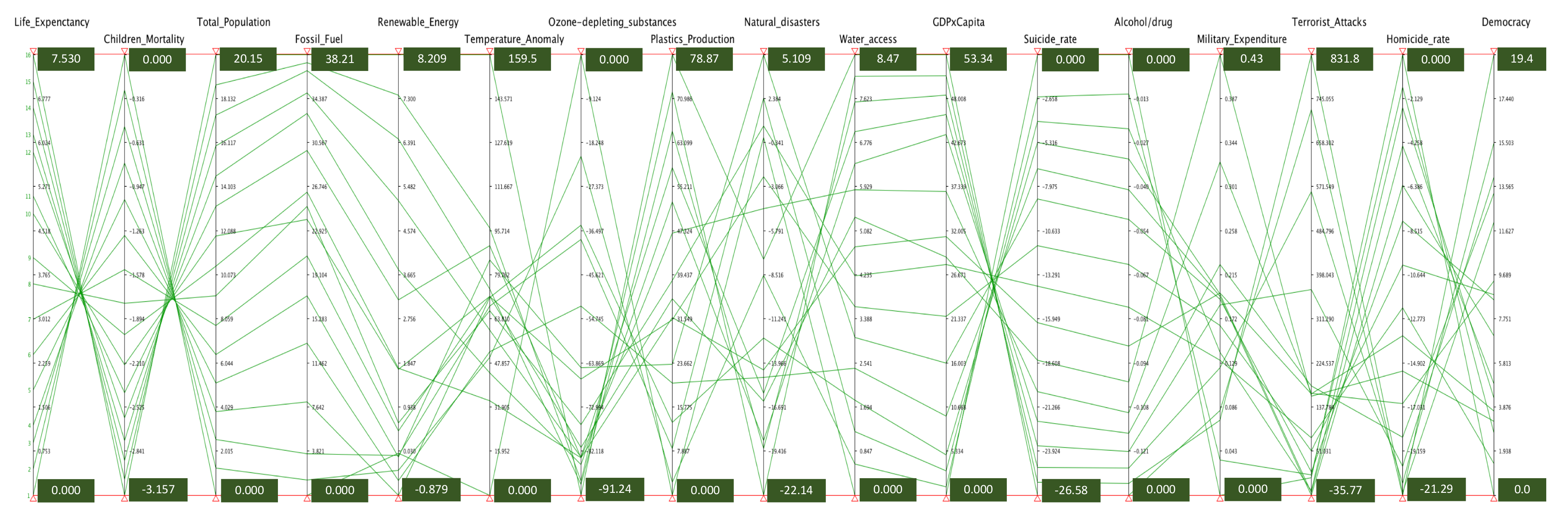
In order to consider the indicator framework as a whole, we have adopted parallel coordinates [61]. Figure 5 shows target indicators. Such a representation has been produced by using XDAT (XDAT—A free parallel coordinates software. https://www.xdat.org.).
Each line represents a year, while each dimension is associated with a different indicator. Indicators are represented as a percentage of variation with respect to the initial state (Equation (2)). For each indicator, we have highlighted the range of the variation. So, for example, the variation of the indicator Democracy (last dimension) is in the range between 0 and 19.4%. Although multi-dimensional data visualization techniques may facilitate the understanding as a whole, they cannot support an actual and proper multi-criteria analysis that requires the combination of indicators to produce some metrics.
6. How Is the World Performing?
In this section, we propose a number of experiments and the discussion of the related computation outputs. The MCDA framework proposed in this paper is purely quantitative as it is based on the combination of numerical indicators. In this section, we focus on interpretations in context to provide a balance between quantitative and qualitative aspects.
In the first experiment proposed, we have adopted random weights, while the second one is based on two real opinions. The main purpose of this section is to show examples of analysis and possible interpretations.
6.1. Some Random Experiments
By adopting the indicator framework previously proposed, we have performed a number of experiments in which the weights associated to the different indicators are randomly generated. As an example, we discuss two experiments that consist of 5 and 50 random samples respectively. The former is the typical size of a small group; for instance, students are often organized in small groups for discussions and/or to perform their assignments or projects. The latter is normally the size of a whole class at a Master level. Average weights are reported in Figure 6.
Regardless of the proportions, the first experiment presents averagely a higher trust in the indicators (5/10 against 4.5/10) as shown by the red bars in the figure. It means that in the first experiment the selected set of indicators is considered more relevant by users than in the second one to measure World performance. We consider the relevance of the selected indicators as a key factor to understand the analysis results in context.
6.2. Computation and Interpretations
Figure 7 presents the results for 5 and 50 random samples. Looking at the left-side charts, each dark green line represents a different computation, while the blue line refers to the computation adopting the average weights. Finally, the light green line proposes the neutral computation as previously described. The right side charts shown again the average computation (blue line) both with the ideal computations corresponding to the most optimist and pessimistic possible trends.
Neutral computation provides an understanding of the indicator framework assuming a neutral approach to indicators’ weights. As shown in the picture, selected indicators are relatively balanced in the period 2000–2011 with some positive trend but they have a clearly negative trend starting from 2011. Looking at the input, the clear factors that are determining such a trend are the temperature anomaly and the terrorist attacks, which have been dramatically increasing in the period. We believe that is a realistic interpretation of the reality in which other factors (e.g., population living in democracy) point to a general improving of life in many aspects but cannot compensate such global phenomena. The method preserves numerical differences among indicators as it does not adopt normalizations or other kind of manipulations. In this specific case, the relevance of the temperature anomaly and of terrorist attacks is directly reflected in measures and such anomaly is re-proposed in the output.
Looking at single samples, they are distributed in a positive, neutral and negative range. The computation based on average values shows a negative performance since 2014 for the smaller experiment and since 2012 for the other one.
Both experiments point out a negative trend. Despite that, the computation shows in this case a moderate optimism. Indeed, much more pessimistic performance is possible in theory looking at that set of indicators (right-side charts) and, above all, average computation shows better performance than neutral computation.
6.3. Computing Real Opinions
We report two additional experiments based on the weights from two different persons (Figure 8). The purpose of this experiment is to compute weights that reflect real opinions. Real opinions on a large scale to perform statistically relevant experiments will be collected in future research. Both of them show a fundamental lack of interest for economy-related indicators focusing mostly on socio-environmental aspects. Regardless of the differences in the proportions proposed, overall one relies much more on the indicator set proposed.
According to those inputs, computations show an evident negative trend for the World performance (Figure 9) with a fundamental pessimism that is much more marked for the person that trust indicators the most. Again, the temperature anomaly plays an important role. In this case, it becomes the main driver factor as it is considered a top-priority (10/10) in both samples. Moreover, unlike the previous example, there is a total lack of interest in aspects that propose a clearly positive trend, such as the GDP and life expectancy. It determines a further decreasing of performance. However, the actual difference between the two users is made by the terrorist attacks that are not considered relevant at all by the second user.
The example proposed shows the sensitiveness of the method to the input weights associated with the different indicators.
7. Current Limitations
Current limitations can be summarized as follows:
- The method does not consider relatedness and redundancy among variables. As discussed in several contributions, e.g., in [62], dependencies and other relationships among variables may play a significant role in terms of correctness and accuracy. In this specific context that assumes global indicators, we believe that the impact of such a limitation is very limited, probably null in most cases.
- Limited semantics. As previously discussed, the semantics associated with the different indicators are very limited and uniquely consist of a wished behaviour. That is a functional requirement rather than a proper semantic. As a consequence, the method is purely numeric and doesn’t allow semantic analysis.
- The method does not deal with uncertainty. The kind of analysis performed is likely to face some uncertainty, such as lack of data and non-numerical indicators. The current development is explicitly oriented to optimize the trade-off between analysis effectiveness and usability.
- Tool implementation. Simplicity is considered the key factor to make the method usable in practice. This philosophy is reflected in the implementation of the tool, whose interface is designed to be suitable to any user. As a consequence, certain kind of analysis technically supported (e.g., multi-dimensional) cannot be performed automatically but needs the manual selection of the input and the generation of the output associated.
At a more practical level, the attempt to simplify a complex analysis in a way that can be suitable to most users is an intrinsic risk. indeed, the method adopts an unique metric resulting from the combination of the different criteria. Although the tuning mechanism makes the method adaptive to the input dataset, the method is still very sensitive of the weights associated with the different indicators. Generally speaking, all indicators are considered reliable and accurate and it is very unlikely that users are expert in the different areas. The method properly works and supports the decision making process under the assumption that clear decisions in input are taken by users weighting the indicators.
8. Conclusions and Future Work
We have proposed a method based on classical MCDA techniques that systematically combines heterogeneous indicators into a unique metric adopted to estimate the performance of the World according to a number of weighted selected criteria.
As extensively discussed in the paper, such a method allows to arbitrary select whichever set of indicators, to weight each indicator and to enrich it by associating relatively simple semantics. Such a performance metric provides a combined understanding of performance, whose interpretation takes into account of the input dataset, of the semantics associated and of the input weights.
The experiments performed show examples of analysis in context. First of all, from a simple analysis of the input weights, it is possible to infer the estimation of the relevance of the considered indicators by users to answer the research question object of this paper. Furthermore, because of the adaptive approach, the interpretation of numerical computations is performed in terms of pessimism/optimism rather than in absolute terms.
In conclusion, we consider the research question object of this paper hard to be answered without a clear understanding of the context in which such a question is formulated. We believe that our adaptive approach can mitigate possible negative effects of pure data-driven analysis by providing a reasonable tool for analysis and interpretation in context.
Future work will extend the computational method to explicitly model biases [63] and uncertainty [64]. Additionally, it should support lack of data and extended semantics (e.g., dependencies among indicators), as well as indicators with non-numerical values. We have not included those advanced features in the base version of the method proposed in the paper because, although the analysis capabilities would result probably extended, they add a significant complexity. Such a complexity would strongly affect the input parameters in such a way to be suitable for experts only. Indeed, we believe that one of the strengths of our tool is its simplicity which allows almost any user to select target indicators, to associate with each of them a wished trend and a weight and to compute the result. We consider this delicate trade-off between analysis capabilities and usability as a key issue for the practical application of the method. A survey on selected communities—i.e., university staff and students - as well as on a large scale will be conducted to estimate the weights associated with the different indicators within the different communities.
Funding
No external funding.
Acknowledgments
I would like to thank Alexey Voinov for revising an early version of this paper and for the interesting conversations on the topic that provided insight and inspired possible future work. I also thank the anonymous reviewers who provided extensive and constructive feedback. It led to an improved version of the paper.
Conflicts of Interest
The author declares no conflict of interest.
References
- Dale, V.H.; Kline, K.L. Issues in using landscape indicators to assess land changes. Ecol. Indic. 2013, 28, 91–99. [Google Scholar] [CrossRef]
- Janssen, M.; Charalabidis, Y.; Zuiderwijk, A. Benefits, adoption barriers and myths of open data and open government. Inf. Syst. Manag. 2012, 29, 258–268. [Google Scholar] [CrossRef] [Green Version]
- Head, B.W. Three lenses of evidence-based policy. Aust. J. Public Adm. 2008, 67, 1–11. [Google Scholar] [CrossRef]
- Rottenburg, R.; Merry, S.E.; Park, S.J.; Mugler, J. The World of Indicators: The Making of Governmental Knowledge Through Quantification; Cambridge University Press: Cambridge, UK, 2015. [Google Scholar]
- Ishizaka, A.; Nemery, P. Multi-Criteria Decision Analysis: Methods and Software; John Wiley & Sons: Hoboken, NJ, USA, 2013. [Google Scholar]
- Merry, S.E.; Conley, J.M. Measuring the world: Indicators, human rights, and global governance. Curr. Anthropol. 2011, 52. [Google Scholar] [CrossRef]
- Jasch, C. Environmental performance evaluation and indicators. J. Clean. Prod. 2000, 8, 79–88. [Google Scholar] [CrossRef]
- Pileggi, S.F.; Hunter, J. An ontological approach to dynamic fine-grained Urban Indicators. Procedia Comput. Sci. 2017, 108, 2059–2068. [Google Scholar] [CrossRef]
- Velasquez, M.; Hester, P.T. An analysis of multi-criteria decision making methods. Int. J. Oper. Res. 2013, 10, 56–66. [Google Scholar]
- Wang, J.J.; Jing, Y.Y.; Zhang, C.F.; Zhao, J.H. Review on multi-criteria decision analysis aid in sustainable energy decision-making. Renew. Sustain. Energy Rev. 2009, 13, 2263–2278. [Google Scholar] [CrossRef]
- Pohekar, S.; Ramachandran, M. Application of multi-criteria decision making to sustainable energy planning—A review. Renew. Sustain. Energy Rev. 2004, 8, 365–381. [Google Scholar] [CrossRef]
- Huang, I.B.; Keisler, J.; Linkov, I. Multi-criteria decision analysis in environmental sciences: ten years of applications and trends. Sci. Total. Environ. 2011, 409, 3578–3594. [Google Scholar] [CrossRef]
- Linkov, I.; Varghese, A.; Jamil, S.; Seager, T.P.; Kiker, G.; Bridges, T. Multi-criteria decision analysis: A framework for structuring remedial decisions at contaminated sites. In Comparative Risk Assessment and Environmental Decision Making; Springer: Berlin/Heidelberg, Germany, 2004; pp. 15–54. [Google Scholar]
- Baltussen, R.; Niessen, L. Priority setting of health interventions: the need for multi-criteria decision analysis. Cost Eff. Resour. Alloc. 2006, 4, 14. [Google Scholar] [CrossRef] [PubMed] [Green Version]
- Nutt, D.J.; King, L.A.; Phillips, L.D. Drug harms in the UK: A multicriteria decision analysis. Lancet 2010, 376, 1558–1565. [Google Scholar] [CrossRef]
- Malczewski, J. GIS-based multicriteria decision analysis: A survey of the literature. Int. J. Geogr. Inf. Sci. 2006, 20, 703–726. [Google Scholar] [CrossRef]
- Kiker, G.A.; Bridges, T.S.; Varghese, A.; Seager, T.P.; Linkov, I. Application of multicriteria decision analysis in environmental decision making. Integr. Environ. Assess. Manag. 2005, 1, 95–108. [Google Scholar] [CrossRef] [PubMed]
- Linkov, I.; Satterstrom, F.K.; Kiker, G.; Batchelor, C.; Bridges, T.; Ferguson, E. From comparative risk assessment to multi-criteria decision analysis and adaptive management: Recent developments and applications. Environ. Int. 2006, 32, 1072–1093. [Google Scholar] [CrossRef] [PubMed]
- Phillips, L.D.; e Costa, C.A.B. Transparent prioritisation, budgeting and resource allocation with multi-criteria decision analysis and decision conferencing. Ann. Oper. Res. 2007, 154, 51–68. [Google Scholar] [CrossRef] [Green Version]
- Gandomi, A.; Haider, M. Beyond the hype: Big data concepts, methods, and analytics. Int. J. Inf. Manag. 2015, 35, 137–144. [Google Scholar] [CrossRef] [Green Version]
- Suciu, G.; Anwar, M.; Rogojanu, I.; Pasat, A.; Stanoiu, A. Big data technology for scientific applications. In Proceedings of the 2018 Conference Grid, Cloud & High Performance Computing in Science (ROLCG), Cluj-Napoca, Romania, 17–19 October 2018; pp. 1–4. [Google Scholar]
- Ait-Mlouk, A.; Agouti, T.; Gharnati, F. Mining and prioritization of association rules for big data: multi-criteria decision analysis approach. J. Big Data 2017, 4, 42. [Google Scholar] [CrossRef] [Green Version]
- Blanco-Mesa, F.; Merigó, J.M.; Gil-Lafuente, A.M. Fuzzy decision making: A bibliometric-based review. J. Intell. Fuzzy Syst. 2017, 32, 2033–2050. [Google Scholar] [CrossRef] [Green Version]
- Klein, G. Naturalistic decision making. Hum. Factors 2008, 50, 456–460. [Google Scholar] [CrossRef] [Green Version]
- Jiang, Y.; Liu, H.; Tang, Y.; Chen, Q. Semantic decision making using ontology-based soft sets. Math. Comput. Model. 2011, 53, 1140–1149. [Google Scholar] [CrossRef]
- Zhang, C.; Zhou, G.; Lu, Q.; Chang, F. Graph-based knowledge reuse for supporting knowledge-driven decision-making in new product development. Int. J. Prod. Res. 2017, 55, 7187–7203. [Google Scholar] [CrossRef]
- Ritchie, H.; Roser, M. CO2 and other Greenhouse Gas Emissions. Our World in Data. 2019. Available online: https://ourworldindata.org/co2-and-other-greenhouse-gas-emissions (accessed on 20 March 2019).
- Morice, C.P.; Kennedy, J.J.; Rayner, N.A.; Jones, P.D. Quantifying uncertainties in global and regional temperature change using an ensemble of observational estimates: The HadCRUT4 data set. J. Geophys. Res. Atmos. 2012, 117. [Google Scholar] [CrossRef]
- Ritchie, H.; Roser, M. Ozone Layer. Our World in Data. 2019. Available online: https://ourworldindata.org/ozone-layer (accessed on 20 March 2019).
- Agency, E.E. Consumption of Controlled Ozone-Depleting Substances. Available online: https://www.eea.europa.eu/data-and-maps/daviz/consumption-of-controlled-ozone-depleting-substances#tab-chart_1 (accessed on 20 March 2019).
- Ritchie, H.; Roser, M. Plastic Pollution. Our World in Data. 2019. Available online: https://ourworldindata.org/plastic-pollution (accessed on 20 March 2019).
- Geyer, R.; Jambeck, J.R.; Law, K.L. Production, use, and fate of all plastics ever made. Sci. Adv. 2017, 3, e1700782. [Google Scholar] [CrossRef] [PubMed] [Green Version]
- Ritchie, H.; Roser, M. Natural Disasters. Our World in Data. 2019. Available online: https://ourworldindata.org/natural-disasters (accessed on 20 March 2019).
- Université Catholique de Louvain–Brussels–Belgium. EMDAT (2019): OFDA/CRED International Disaster Database. Available online: http://www.emdat.be/ (accessed on 20 March 2019).
- Ritchie, H.; Roser, M. Water Use and Sanitation. Our World in Data. 2019. Available online: https://ourworldindata.org/water-use-sanitation (accessed on 20 March 2019).
- Bank, W. World Development Indicators. Available online: http://data.worldbank.org/data-catalog/world-development-indicators (accessed on 20 March 2019).
- Roser, M. Life Expectancy. Our World in Data. 2019. Available online: https://ourworldindata.org/life-expectancy (accessed on 20 March 2019).
- WHO. Life Expectancy Data. Available online: http://apps.who.int/gho/data/node.main.688 (accessed on 20 March 2019).
- Bank, W. World Development Indicators (WDI). Available online: https://data.worldbank.org/indicator/SP.DYN.LE00.IN (accessed on 20 March 2019).
- Roser, M. Child Mortality. Our World in Data. 2019. Available online: https://ourworldindata.org/child-mortality (accessed on 20 March 2019).
- Gapminder. Child Mortality. Available online: https://www.gapminder.org/data/documentation/gd005/ (accessed on 20 March 2019).
- Division, T.U.N.P. UN Population Division Data. Available online: https://population.un.org/wpp/Download/Standard/Interpolated/ (accessed on 20 March 2019).
- Roser, M.; Ortiz-Ospina, E. World Population Growth. Our World in Data. 2019. Available online: https://ourworldindata.org/world-population-growth (accessed on 20 March 2019).
- United Nations, D.O.E.; Social Affairs, P.D. World Population Prospects: The 2017 Revision. Available online: https://population.un.org/wpp/Download/Standard/Population/ (accessed on 20 March 2019).
- Lindsay Lee, M.R.; Ortiz-Ospina, E. Suicide. Our World in Data. 2019. Available online: https://ourworldindata.org/suicide (accessed on 20 March 2019).
- GHDx. Global Burden of Disease Collaborative Network. Global Burden of Disease Study 2016 (GBD 2016) Results. Available online: http://ghdx.healthdata.org/gbd-results-tool (accessed on 20 March 2019).
- Ritchie, H.; Roser, M. Substance Use. Our World in Data. 2019. Available online: https://ourworldindata.org/substance-use (accessed on 20 March 2019).
- Roser, M. Economic Growth. Our World in Data 2019. Available online: https://ourworldindata.org/economic-growth (accessed on 20 March 2019).
- Bolt, J.; Van Zanden, J.L. The Maddison Project: Collaborative research on historical national accounts. Econ. Hist. Rev. 2014, 67, 627–651. [Google Scholar] [CrossRef] [Green Version]
- Bolt, J.; Inklaar, R.; de Jong, H.; van Zanden, J.L. Maddison Project Database, Version 2018. Rebasing ‘Maddison’: New Income Comparisons and the Shape of Long-Run Economic Development, Maddison Project Working Paper 10. Available online: https://www.rug.nl/ggdc/historicaldevelopment/maddison/releases/maddison-project-database-2018 (accessed on 20 March 2019).
- Ritchie, H.; Roser, M. Fossil Fuels. Our World in Data. 2019. Available online: https://ourworldindata.org/fossil-fuels (accessed on 20 March 2019).
- Smil, V. Energy Transitions: Global and National Perspectives; ABC-CLIO: Santa Barbara, CA, USA, 2016. [Google Scholar]
- BP. BP Statistical Review of World Energy. Available online: http://www.bp.com/statisticalreview (accessed on 20 March 2019).
- Ritchie, H.; Roser, M. Renewable Energy. Our World in Data. 2019. Available online: https://ourworldindata.org/renewable-energy (accessed on 20 March 2019).
- Roser, M.; Nagdy, M. Military Spending. Our World in Data. 2019. Available online: https://ourworldindata.org/military-spending (accessed on 20 March 2019).
- SIPRI. Yearbook: Armaments, Disarmament and International Security. Available online: https://datacatalog.worldbank.org/dataset/world-development-indicators (accessed on 20 March 2019).
- Max Roser, M.N.; Ritchie, H. Terrorism. Our World in Data. 2019. Available online: https://ourworldindata.org/terrorism (accessed on 20 March 2019).
- Global Terrorism Database (GTD). Available online: https://www.start.umd.edu/gtd/ (accessed on 20 March 2019).
- Roser, M. Homicides. Our World in Data. 2019. Available online: https://ourworldindata.org/homicides (accessed on 20 March 2019).
- Roser, M. Democracy. Our World in Data. 2019. Available online: https://ourworldindata.org/democracy (accessed on 20 March 2019).
- Inselberg, A.; Dimsdale, B. Parallel coordinates: A tool for visualizing multi-dimensional geometry. In Proceedings of the 1st conference on Visualization’90, San Francisco, CA, USA, 23–26 October 1990; IEEE Computer Society Press: Washington, DC, USA, 1990; pp. 361–378. [Google Scholar]
- Servadio, J.L.; Convertino, M. Optimal information networks: Application for data-driven integrated health in populations. Sci. Adv. 2018, 4, e1701088. [Google Scholar] [CrossRef] [Green Version]
- Hämäläinen, R.P.; Alaja, S. The threat of weighting biases in environmental decision analysis. Ecol. Econ. 2008, 68, 556–569. [Google Scholar] [CrossRef]
- Durbach, I.N.; Stewart, T.J. Modeling uncertainty in multi-criteria decision analysis. Eur. J. Oper. Res. 2012, 223, 1–14. [Google Scholar] [CrossRef]
Figure 1.
Graphical representation of tuning.

Figure 2.
Input interface.

Figure 3.
Tuning examples.


Figure 4.
Global indicators by category.

Figure 5.
Indicator framework represented in parallel coordinates.

Figure 6.
Average weights corresponding to 5 and 50 random samples.

Figure 7.
Computation results related to 5 and 50 random samples.

Figure 8.
Two sets of weights showing a fundamental lack of interest for economy-related indicators with a priority on socio-environmental aspects. Overall, the set on the top relies much more on the indicator set proposed (7.5/10 versus 5.5/10).
Figure 8.
Two sets of weights showing a fundamental lack of interest for economy-related indicators with a priority on socio-environmental aspects. Overall, the set on the top relies much more on the indicator set proposed (7.5/10 versus 5.5/10).

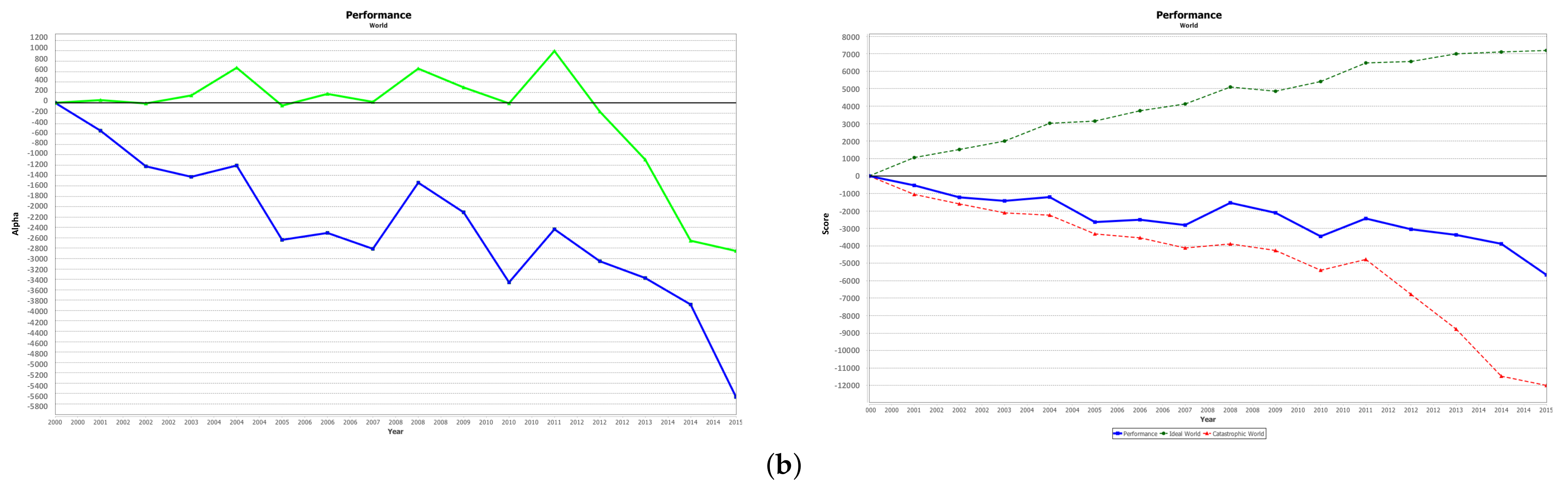
Figure 9.
Computation outputs based on real weights. Both show a negative trend with a fundamental pessimism. It is more marked for the person that trust indicators the most (experiment on top). (a) Computation associated with the preferences that show higher trust on the indicator set proposed; (b) Computation associated with the preferences that show lower trust on the indicator set proposed.


Table 1.
Systematic comparison of the different decision making techniques considering four different selection criteria.
Table 1.
Systematic comparison of the different decision making techniques considering four different selection criteria.
| Technique/Method | Realistic/Data Availability | Easy to Apply/Use | Unbiased | Low Cost |
|---|---|---|---|---|
| Big Data | ** | * | *** | * |
| Fuzzy decision making | *** | * | ** | *** |
| Naturalistic decision making | ** | *** | * | * |
| Semantic decision making | ** | *** | ** | * |
| MCDA | *** | *** | ** | *** |
(*) = low, (**) = medium, (***) = high.
Table 2.
Indicator framework.
| Indicator | Description | Expected Trend () | Reference/Data Source |
|---|---|---|---|
| Environment | |||
| Temperature Anomaly | Global average land-sea temperature anomaly. | DECREASING | [27,28] |
| Consumption of ozone-depleting substances | Global consumption of ozone-depleting substances. | DECREASING | [29,30] |
| Plastics Production | Annual plastics production. | DECREASING | [31,32] |
| Natural Disasters ine Access to improved drinking water | Number of natural disaster events. Share of the population with access to improved drinking water. | DECREASING INCREASING | [33,34] [35,36] |
| Population | |||
| Life Expectancy | Life expectancy at birth. | INCREASING | [37,38,39] |
| Child Mortality | Share dying in first 5 years (%). | DECREASING | [40,41,42] |
| Total Population | Total Population. | DECREASING | [43,44] |
| Health | |||
| Suicide rate | Suicides per 100,000 people. | DECREASING | [45,46] |
| Alcohol or drug use disorder | Population with alcohol or drug use disorders. Tobacco is not included. | DECREASING | [46,47] |
| Growth & Inequality | |||
| GDP per capita | Real GDP per capita with inflation adjusted at 2011. | INCREASING | [48,49,50] |
| Energy | |||
| Fossil Fuels Consumption | Fossil fuel consumption. | DECREASING | [51,52,53] |
| Renewable Energy Consumption | Renewable Energy consumption. | INCREASING | [52,53,54] |
| War and Peace | |||
| Military Expendure | Military Expendure as a share of GDP. | DECREASING | [55,56] |
| Terroristic Attacks | Number of terroristic attacks. | DECREASING | [57,58] |
| Violence and Rights | |||
| Homicide rate | Number of homicide deaths per 100,000 people. | DECREASING | [46,59] |
| Politics | |||
| Population in Democracy | Population living in democracy. | INCREASING | [60] |
Table 3.
Formal definition of symbols.
| Symbol | Definition |
|---|---|
| A | Indicators matrix. |
| Value of the indicator m at the time n. | |
| Indicators matrix whose values are expressed as a percentage of variation with respect to the initial state. | |
| Value of the indicator m at the time n expressed as a percentage of variation with respect to the initial state. | |
| W | Weights vector. |
| Weight associated with the indicator m. | |
| Preferred behaviour associated with the indicator m. See Table 4 | |
| Evaluation metric resulting by the linear combination of the indicators. | |
| computed assuming | |
| Average of all possible weight values. | |
| Tuning vector. | |
| Value of the tuning vector associated with the indicator i. | |
| that adopts the tuning vector | |
| Weight associated with the the indicator i after tuning. | |
| Extreme computations (superior limit). | |
| Extreme computations (inferior limit). | |
| Extreme computations after tuning. |
Table 4.
Semantics associated with indicators.
| Value | |
|---|---|
| Increasing | +1 |
| Decreasing | −1 |
| ine Stable | +1 if |
| −1 otherwise | |
| ine Stable-increasing | +1 if |
| −1 otherwise | |
| ine Stable-decreasing | +1 if |
| −1 otherwise |
© 2019 by the author. Licensee MDPI, Basel, Switzerland. This article is an open access article distributed under the terms and conditions of the Creative Commons Attribution (CC BY) license (http://creativecommons.org/licenses/by/4.0/).
Share and Cite
MDPI and ACS Style
Pileggi, S.F. Is the World Becoming a Better or a Worse Place? A Data-Driven Analysis. Sustainability 2020, 12, 88. https://doi.org/10.3390/su12010088
AMA Style
Pileggi SF. Is the World Becoming a Better or a Worse Place? A Data-Driven Analysis. Sustainability. 2020; 12(1):88. https://doi.org/10.3390/su12010088
Chicago/Turabian StylePileggi, Salvatore F. 2020. "Is the World Becoming a Better or a Worse Place? A Data-Driven Analysis" Sustainability 12, no. 1: 88. https://doi.org/10.3390/su12010088
Note that from the first issue of 2016, this journal uses article numbers instead of page numbers. See further details here.