Using Machine Learning-Based Algorithms to Analyze Erosion Rates of a Watershed in Northern Taiwan


1
Dept. of Civil Engineering, National Taipei University of Technology, Taipei 10608, Taiwan
2
Disaster Prevention Technology Research Center, Sinotech Engineering Consultants, Taipei 11494, Taiwan
3
Faculty of Engineering, King Mongkut’s Institute of Technology Ladkrabang, Bangkok 10520, Thailand
*
Authors to whom correspondence should be addressed.
Sustainability 2020, 12(5), 2022; https://doi.org/10.3390/su12052022
Submission received: 14 February 2020
/
Revised: 2 March 2020
/
Accepted: 4 March 2020
/
Published: 6 March 2020
(This article belongs to the Special Issue Soil Erosion and Sustainable Land Management (SLM))
Abstract
:This study continues a previous study with further analysis of watershed-scale erosion pin measurements. Three machine learning (ML) algorithms—Support Vector Machine (SVM), Adaptive Neuro-Fuzzy Inference System (ANFIS), and Artificial Neural Network (ANN)—were used to analyze depth of erosion of a watershed (Shihmen reservoir) in northern Taiwan. In addition to three previously used statistical indexes (Mean Absolute Error, Root Mean Square of Error, and R-squared), Nash–Sutcliffe Efficiency (NSE) was calculated to compare the predictive performances of the three models. To see if there was a statistical difference between the three models, the Wilcoxon signed-rank test was used. The research utilized 14 environmental attributes as the input predictors of the ML algorithms. They are distance to river, distance to road, type of slope, sub-watershed, slope direction, elevation, slope class, rainfall, epoch, lithology, and the amount of organic content, clay, sand, and silt in the soil. Additionally, measurements of a total of 550 erosion pins installed on 55 slopes were used as the target variable of the model prediction. The dataset was divided into a training set (70%) and a testing set (30%) using the stratified random sampling with sub-watershed as the stratification variable. The results showed that the ANFIS model outperforms the other two algorithms in predicting the erosion rates of the study area. The average RMSE of the test data is 2.05 mm/yr for ANFIS, compared to 2.36 mm/yr and 2.61 mm/yr for ANN and SVM, respectively. Finally, the results of this study (ANN, ANFIS, and SVM) were compared with the previous study (Random Forest, Decision Tree, and multiple regression). It was found that Random Forest remains the best predictive model, and ANFIS is the second-best among the six ML algorithms.
1. Background and Introduction
Soil erosion is of major concern to agriculture and has had a detrimental long-term effect on both soil productivity and the sustainability of agriculture in particular. Soil erosion can lead to water pollution, increased flooding, and sedimentation, which damage the environment [1]. This has influenced the introduction of erosion control practices and policies as a necessity in almost every country of the world and under virtually every type of land use. Soil erosion causes both on-site and off-site consequences [2]. The on-site effects, such as soil losses from a field and depleted organic matter or nutrients of the soil, are particularly relevant on agricultural land. Off-site, downstream sedimentation decreases the capacity of rivers and reservoirs, increasing the threat from flooding. Many hydroelectricity and irrigation projects have been ruined as a consequence of soil erosion [3].
In Taiwan, 74% of the land area is slopes. Moreover, the average annual rainfall amount is 2500 mm, mainly occurred from May to August. As a result of climate change, and the concentration of rainfall duration and increasing rainfall intensity, year-round water availability has become a critical issue in Taiwan. Most of the soil erosion in Taiwan has been the result of unsuitable agricultural behaviors and overuse of slope lands. For example, about 65% of the hillslope lands are for crop production [4]. Coupled with the abundant rainfall, severe soil erosion occurs. Brought into service in 1964, the Shihmen Reservoir ranks third among all reservoirs in the country in terms of storage capacity. However, typhoons cause serious sediment problems and soil erosion [5]. Therefore, a thorough evaluation of the causative factors (predictors) of soil erosion in the watershed is important to the people of Taiwan.
Lo [6] applied the Agricultural Non-Point Source Pollution (AGNPS) model, which simulates water erosion and the transport of sediments to predict sedimentation in the watershed of the Shihmen reservoir. The results showed that the depth of sedimentation in the watershed averages around 2.5 mm/yr. Soil erosion in the watershed was also evaluated using USLE on different Digital Elevation Models (DEMs), and the average annual soil erosion rate varied greatly depending on the DEM [7]. Chiu et al. [8] used 137Cs radionuclide collected from 60 hillslope sampling sites of the basin of the Shihmen reservoir to determine the soil erosion rate and found it to be one or two orders of magnitude lower than predicted by USLE. Recently, Liu et al. [9] improved the analysis of the Shihmen reservoir watershed using the slope unit method in addition to the common grid cell approach. The results were verified with erosion pin measurements.
Erosion pins are a conventional method of measuring soil erosion. Erosion pins have been employed to measure ground-lowering rates and compare erosion rates of rill and interrill areas, plots of different sizes, slope areas, and many other regions in need of study. For example, Sirvent et al. [10] used erosion pins to measure the ground lowering in two plots every six months. The result demonstrated that erosion rates in the rill areas were 25%–50% higher than those in the interrill areas. Edeso et al. [11] used 29 erosion pins to evaluate soil erosion of different plots in northern Spain and showed that soil erosion in all plots was increasing over time. In Taiwan, Lin et al. [12] concluded that the soil erosion depth measured by erosion pins sharply increased when the accumulated rainfall exceeded 200 mm in a rainfall event.
An Artificial Neural Network (ANN) is an artificial intelligence model that was used to process information and was inspired by the human brain [13]. An Adaptive Neuro-Fuzzy Inference System (ANFIS) is an artificial intelligence model that combines neural networks with fuzzy inference systems [14]. The unique structure of ANFIS incorporates the ability of fuzzy inference systems (FIS) to improve the precision of prediction. Finally, SVM (Support Vector Machine) is a machine learning (ML) method that is very suited to intricate classification problems. In recent years, these artificial intelligence techniques have been applied to many different fields [15]. For example, Quej et al. [16] used ANN, ANFIS, and SVM to predict the daily global solar radiation in the Yucatan Peninsula, Mexico. Model performance was evaluated by the Mean Absolute Error (MAE), Root Mean Squared of Error (RMSE), and R-squared (R2). The result indicated that SVM has a better performance than the other techniques. Zhou et al. [17] compared the accuracy of four models including ANN, SVM, WANN (Wavelet preprocessed ANN), and WSVM (Wavelet preprocessed SVM) to predict groundwater depth. The results showed that the models are ranked as follows: WSVM > WANN > SVM > ANN. Angelaki et al. [18] also used ANFIS, ANN, and SVM to predict the cumulative infiltration of soil. The results of model performance based on RMSE and Correlation Coefficient (CC) suggest that ANFIS works better than both SVM and ANN.
In the field of soil erosion modeling, there have been many studies carried out to estimate soil erosion using models such as USLE [9,19], SWAT [20,21], WEPP [22,23], WaTEM/SEDEM [24,25], and EUROSEM [26]. However, there has been no application of ML algorithms to estimate soil erosion except for in our previous work [27], in which we used Decision Tree (DT), Random Forest (RF), and Multiple Regression (MR) to create ML models to predict the soil erosion depths (rates). Therefore, this study aims to extend the investigation to the application of other ML techniques. Our main goal is to further our understanding of soil erosion rates in the study area.
2. Dataset and Research Method
The research design involves the use of site-specific data collected in the study area. They are described in the sections below.
2.1. Area of Study
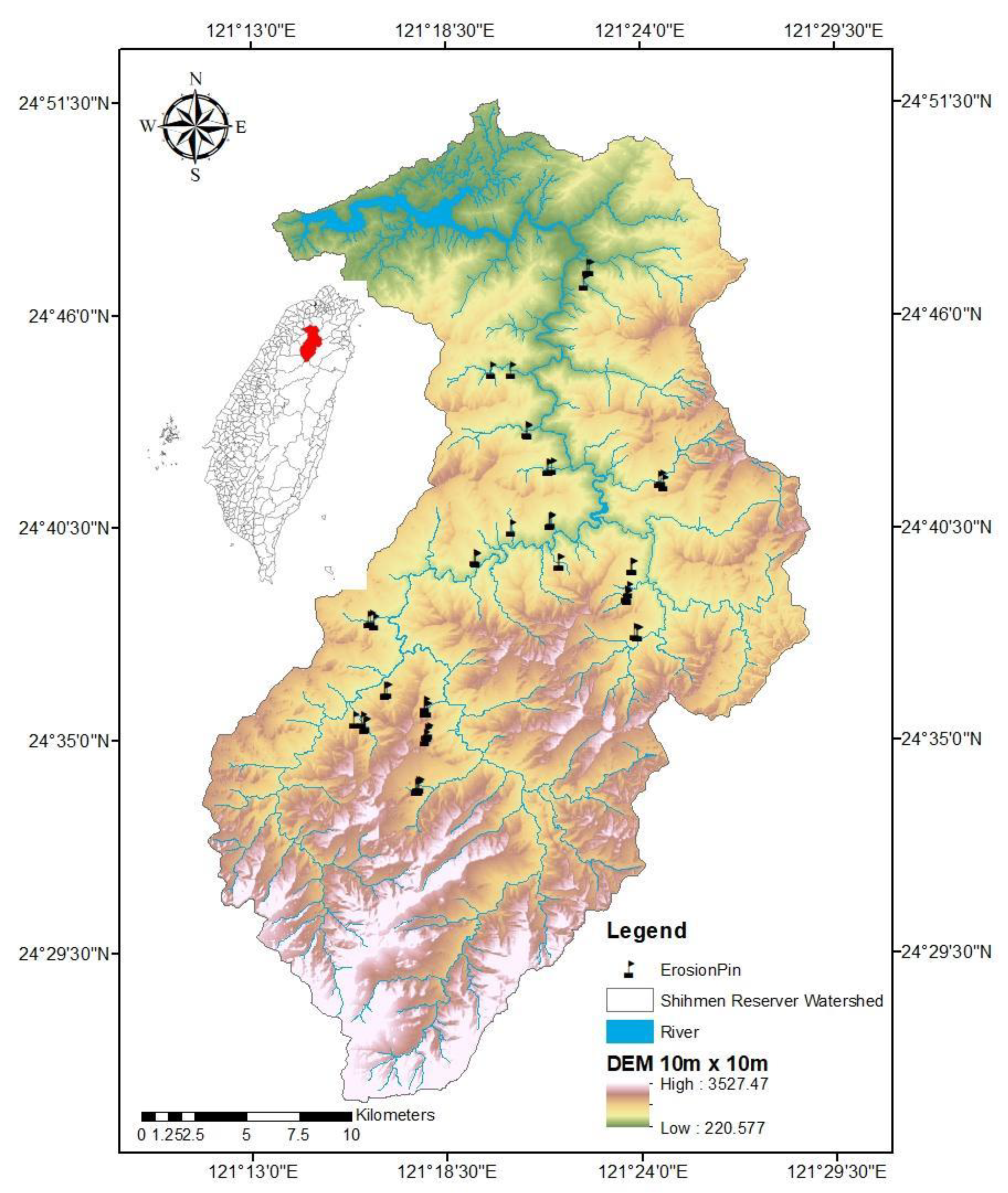
The Shihmen reservoir dam is situated in the northern part of Taiwan on the banks of the Tahan River. Its watershed has an area of approximately 759.53 km2 (Figure 1), and elevation rises towards the south. Hills extend over most areas, and for more than 60% of the watershed, the slope is more than 55% [28]. The yearly average temperature is 19 ℃ and average humidity, 82%. The typical rainy season is from May to October and the dry season from November to April. The average annual precipitation is approximately 2500 mm/yr [28].
2.2. Data Preparation
We collected various data about the locations of the installed erosion pins as well as the measurements of the erosion pins themselves, as described in the following sections.
2.2.1. Predictors
A total of 14 environmental factors were utilized as the predictors (independent factors or input variables) in the model, namely distance to river, distance to road, type of slope, sub-watershed, slope direction, elevation, slope class, rainfall, epoch, lithology, and the amount of organic content, clay, sand, and silt in the soil. These factors have been gathered from different sources and become a geospatial database, as described in Nguyen et al. [27].
2.2.2. Target
The specification and installation of the erosion pins were described in Lin et al. [12]. Within the boundary of the Shihmen reservoir watershed, a total of 550 pins were installed on 55 slopes (10 pins per slope). The measurement data were collected from 8 September 2008 to 10 October 2011. The annual erosion depths were averaged at each slope, and the value ranges from 2.17 to 13.03 mm/yr. The metal rods (pins) used in this analysis were mounted on slopes without any signs of a landslide, collapse, or gully erosion. Therefore, our findings cannot be generalized beyond sheet and rill erosion.
2.3. Model Configuration
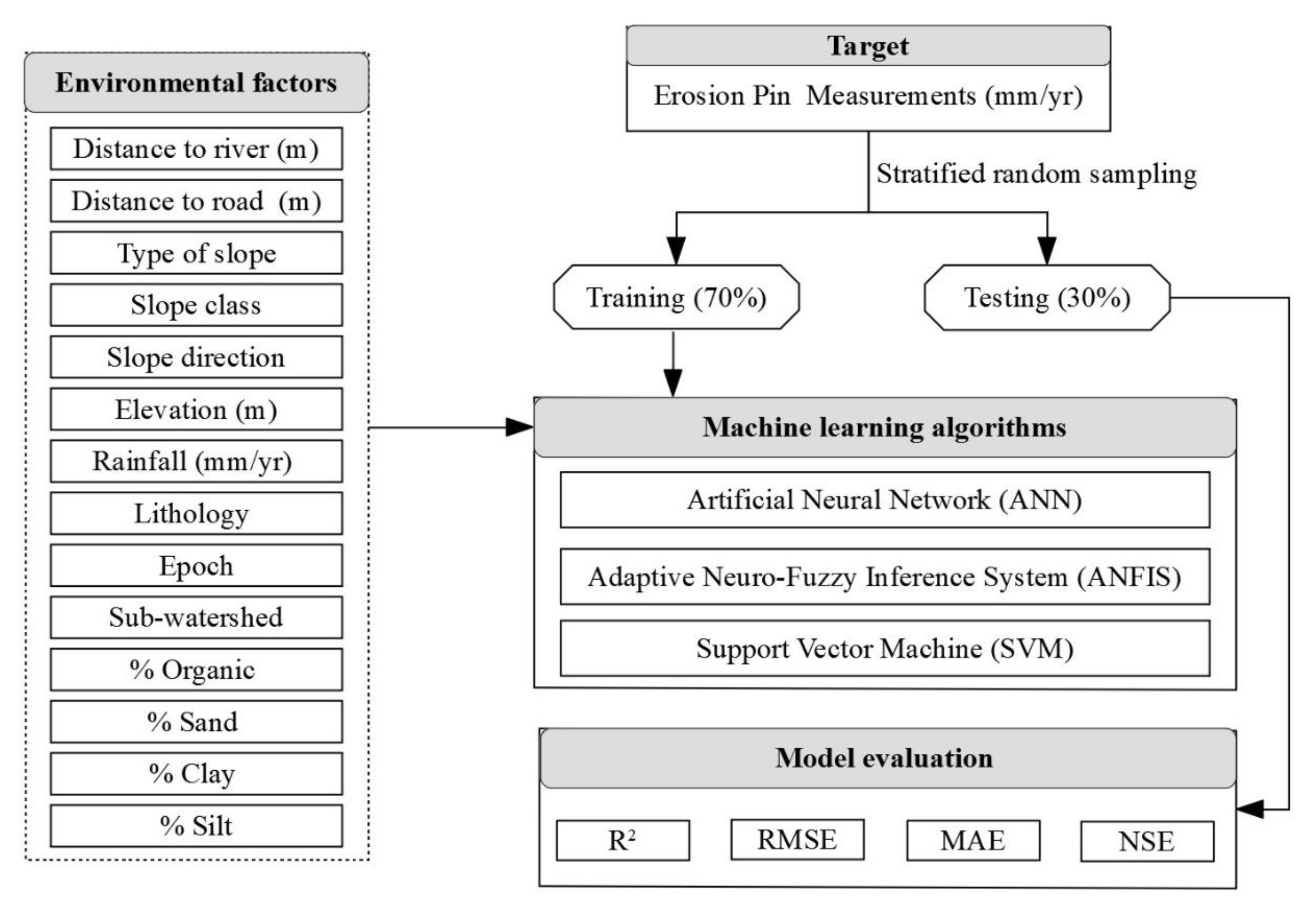
In this study, ML algorithms were used to predict the erosion rates of sheet erosion and rill erosion. The overall framework of the study consisted of three main parts (Figure 2), as summarized below.
First, the entire dataset, which includes 14 predictors and one target, was divided into a training set (70% or 38 samples) and a test set (30% or 17 samples) as is commonly done in the literature [29,30,31,32]. This step was repeated three times (i.e., Grouping #1, Grouping #2, and Grouping #3) to reduce the data variability to sampling. Because stratified random sampling has been shown to produce better outcomes than the simple random sampling [27], only stratified random sampling was used in this study to ensure the proper representation of the population. In stratified random sampling, the dataset was divided into several strata, and each stratum was sampled proportionately (70/30). Sub-watershed was selected as the stratification variable for this study, because it had been shown that the erosion depths in different watersheds were statistically different [33]. Hence, using stratified random sampling with sub-watershed as the stratification variable can provide a better estimate of the sample statistics and therefore create a better ML model.
Second, the ANN, ANFIS, and SVM models were built using the 70% training data, and the resulting models were tested using the test data.
Third, the performance metrics of R2, NSE (Nash–Sutcliffe Efficiency), RMSE, and MAE were calculated on the training and test data. The Wilcoxon signed-rank test was conducted to determine if a statistically significant difference exists between the three models. Finally, the results of ANN, ANFIS, and SVM were tabulated and compared with results from our previous research [27].
2.4. Machine Learning Algorithms
Three widely used and potentially applicable ML algorithms are used in this study. They are described below.
2.4.1. Artificial Neural Network
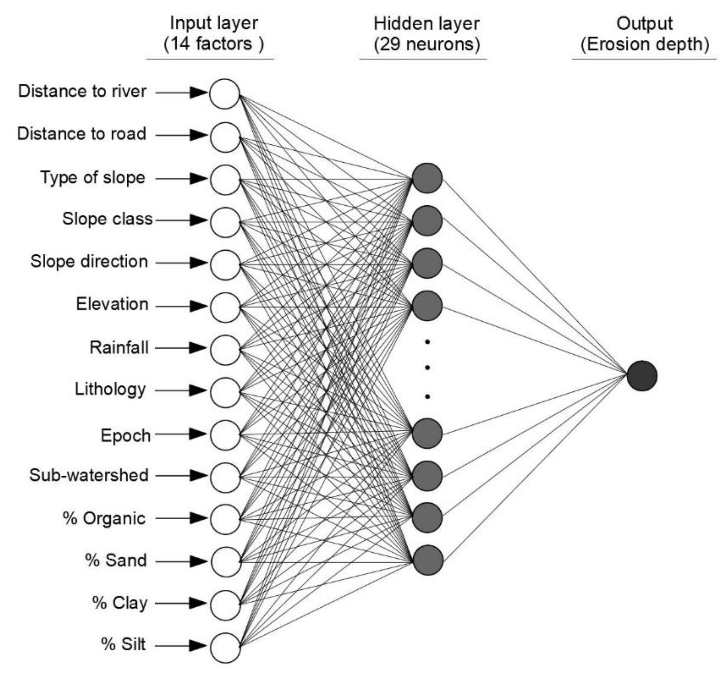
An Artificial Neural Network (ANN) mimics how the human brain processes information. The purpose of the ANN model is to predict a target outcome by using input data through a back-propagation learning algorithm [34]. A typical ANN model has a multi-layer feed-forward structure that is connected by nodes with three main layers, namely the input layer, the hidden layer(s), and the output layer. The ANN determines the weight for each node and builds its results through training. In this study, the ANN model was created using the ‘nntool’ in the MATLAB 2016 software. A three layers feed-forward back-propagation network type was used. It consists of an input layer (14 neurons representing 14 environmental factors), one hidden layer (29 neurons), and one output layer (erosion rate), as shown in Figure 3. The number of neurons of the hidden layer is determined based on the following equation [35]:
where N is the number of hidden nodes, and x is the number of input nodes.
2.4.2. Adaptive Neuro-Fuzzy Inference System
An Adaptive Neuro-Fuzzy Inference System (ANFIS) is a combination of ANN and fuzzy logic, which utilizes the strengths of both techniques. Jang [14] introduced the concept of ANFIS in 1993. ANFIS contains five layers connected by directed links. These five layers are the Fuzzification layer, the Product layer, the Normalized layer, the Defuzzification layer, and the Output layer. The main purpose of ANFIS is to define the optimum parameter values of an equivalent fuzzy inference system by applying a learning algorithm. ANFIS can be constructed using two different methods, namely Genfis 1 (grid partitioning) and Genfis 2 (subtractive clustering). Genfis 1 has a limitation of six input variables. Since we have 14 factors, we used Genfis 2 in our analysis instead of Genfis 1. In this research, the ANFIS model was constructed using the “anfisedit” tool in the MATLAB 2016 software following the steps of loading data, generating FIS (sub clustering), and testing.
2.4.3. Support Vector Machine
A Support Vector Machine (SVM) is a supervised learning model developed by Schölkopf et al. [36] that can be used for regression and classification. The SVM model algorithm creates a line or a hyperplane that divides a dataset into two classes. The distance from the hyperplane to the nearest data points on both sides is defined as the margin. The purpose is to select a hyperplane with the greatest possible margin, thus giving a greater chance of new data being classified correctly into these two classes. In this study, the SVM model was implemented using custom codes and the ‘fitrsvm’ package on the MATLAB 2016 software.
2.5. Evaluation Criteria of Model Performance
Model evaluation is an indispensable part of developing a useful model. It supports the discovery and selection of a good model that can be used in the future. There are several statistical indices commonly used to estimate and calculate the performance and the validity of the ML algorithms. Here, the statistical parameters employed to measure the errors between the predicted and the observed values are R2, NSE, RMSE, and MAE [37,38,39].
The R2 value indicates the consistency with which the predicted values versus the measured values following a regression line [27]. It ranges from zero to one. If the value is equal to one, the predictive model is considered “perfect.” The definition of R2 is as follows:
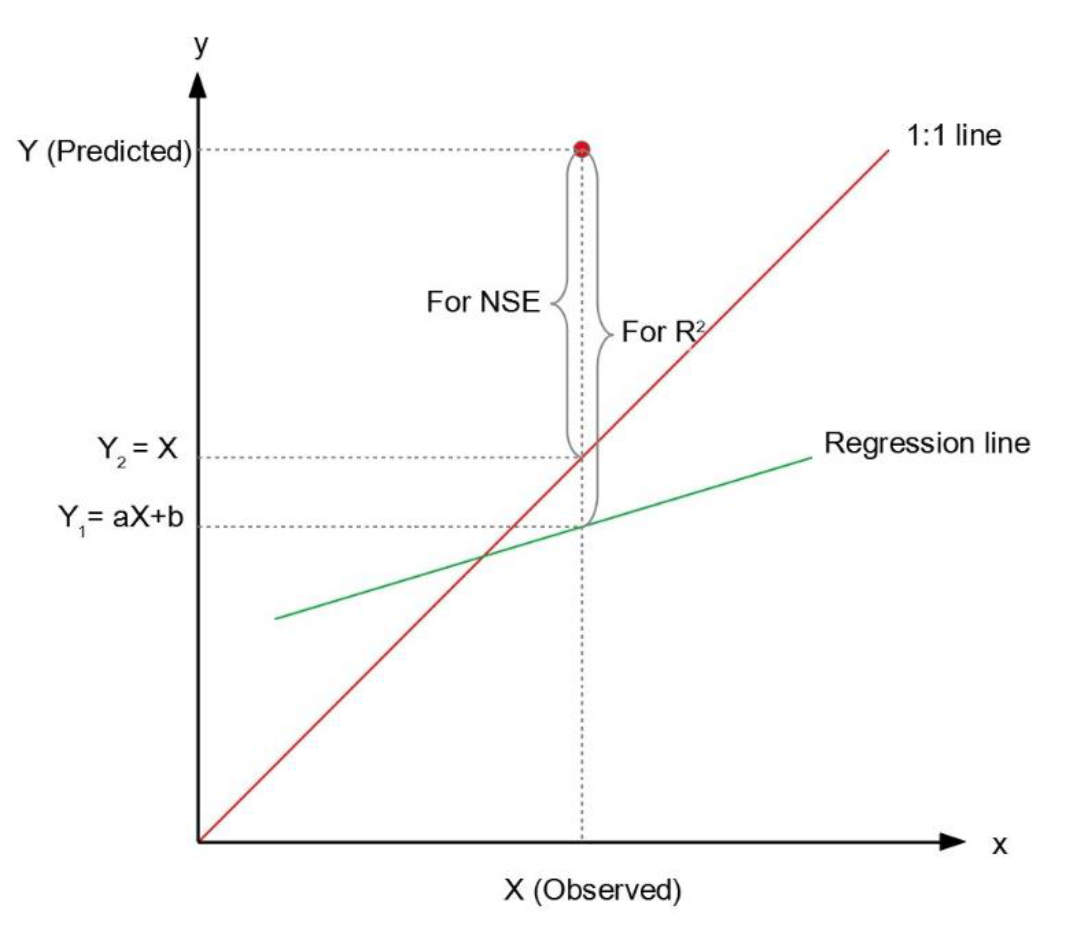
where SST represents the total sum of squares, SSE is the error sum of squares, Y is the prediction of the model, Y1 is the prediction of the regression line, and is the average of predicted values (Figure 4).
It is worth noting that although R2 has been widely used for model evaluation, the statistics are highly sensitive to extreme values and are insensitive to additive and proportional differences between model and measured data [40]. More importantly, R2 is calculated against the regression line (Figure 4), not the 1:1 line. A high R2 only means a good fit to the regression line, not necessarily a set of good predictions concerning the observations (see the distinction made between the regression line and the 1:1 line in Figure 4). Therefore, we retain R2 in this study only for completeness. Instead of relying on R2, we computed RMSE, MAE, and NSE to compare the model performance. They are more appropriate than R2.
RMSE and MAE are statistical parameters that are ‘dimensioned.’ They express the average errors of the model in the unit of the output variable (Equations 3 and 4). The RMSE is of particular importance, because it is one of the most commonly reported parameters in the climatic and environmental literature [41]. Smaller values of RMSE and MAE suggest nearer approximation of observed values by the models. The RSME and MAE are widely used basic metrics for assessing the performance of predictive models [42]. They are defined as follows:
where Y2 is the predicted value of the 1:1 line, and n is the number of samples.
In addition to R2, RMSE, and MAE, which all have been used in our previous study [27], an additional parameter (NSE) is included in this study. As shown in Equation (5), NSE is a normalized statistical parameter that defines the relative magnitude of the residual variance compared to the measured data variance [43]. It shows how well the plot of the predicted values versus the observed values fits the 1:1 line. The value of NSE ranges from −∞ to one, with NSE = 1 being the optimal value. If the value of NSE is between zero and one, the model is said to have acceptable performance (the higher, the better). On the other hand, if the value of NSE is smaller than 0.0, it will indicate that the average of observed values is better than the predicted value, and the model performance is not acceptable [43].
where X is the observed value and is the average of observed values.
2.6. Wilcoxon Signed-Rank Test
In addition to using NSE, RMSE, and MAE to evaluate the effectiveness of the models, it is necessary to examine if the differences in NSE, RMSE, and MAE are statistically significant. In this study, we used the Wilcoxon signed-rank test to compare the errors generated by different predictive models because the Wilcoxon signed-rank test is non-parametric (distribution-free). The steps of the Wilcoxon signed-rank test are as follows: Let denote the observed value, denote the predicted value of model 1, and denote the predictive value of model 2. The absolute error of each prediction is measured (Equations (6) and (7)) by:
To determine whether one model predicts more accurately than the others do, we perform the one-tailed hypothesis test. The null hypothesis is that “Two models have the same predictive error”. The alternative hypothesis is that “The first model has a smaller error than the second model”. In the Wilcoxon signed-rank test, we chose a significance level of 0.05. Then, the decision to whether to reject the null hypothesis or not is based on the resulting p-value. If the p-value is greater than 0.05, it will fail to reject the null hypothesis. Otherwise, if the p-value is less than 0.05, the null hypothesis will be rejected at a confidence level of 95%. In this case, the Wilcoxon signed-rank test is run using the R command wilcox.test.
3. Results and Discussions
We conducted all analyses using the dataset described in Section 2. Our findings are presented in the following sections.
3.1. Evaluation of Predictive Models
This study used quantitative criteria to assess the performance of predictive models. Table 1 shows the computed R2, NSE, RMSE, and MAE statistics for ANFIS, ANN, and SVM under three different stratified random samplings. Among the four parameters, R2 and NSE are statistics used to evaluate the predictive performance of the models under consideration. The higher the R2 and NSE, the better the models simulate the results. However, as shown in Figure 4, R2 is a measure of the goodness-of-fit of the regression line, not the 1:1 line. Therefore, a high R2 does not necessarily mean a good performance of the model for predicting the soil erosion rate. In this regard, NSE is a much more suitable index to use because it is based on the differences between the predicted and observed values (1:1 line). Therefore, in the following, we will restrict our discussion to NSE only and ignore R2.
On the other hand, MAE and RMSE are evaluation metrics commonly used to gauge the performance of the models that output continuous numbers. Both RMSE and MAE produce average errors of the models in units of the model output variables. However, it is worth noting that RMSE and MSE could be calculated against the 1:1 line or the regression line [27], and different results could be obtained. In this study, we computed both RMSE and MSE based on the 1:1 line to reflect the differences between the predicted and observed values.
As can be seen from Table 1, the average NSE of the training data for the ANN, ANFIS, and SVM models is 0.62, 1.00, and 0.51, respectively. Theoretically, the value of NSE ranges from −∞ to one, and the higher the NSE, the better the model performs. Thus, it can be inferred from these numbers that ANFIS is the best model with a perfect NSE value of 1.00, and it outperforms the other two models substantially. However, the average NSE deteriorates significantly when the test data are used to judge the true performance of the models. They are 0.32, 0.49, and 0.17 for the ANN, ANFIS, and SVM models, respectively. The ANFIS model remains the best performing model, while the ANN model still beats the SVM. It is worth noting that a negative NSE was obtained for grouping #2 of SVM. This means that the model did not contribute to the improvement of the prediction, and the average of the observed values is better than the predicted value [44].
According to Table 1, there is also a significant difference in the RMSE values across the three models. The average RMSE of the training data for the ANN, ANFIS, and SVM models is 1.23, 0.01, and 1.43 mm/yr, respectively. Again, the ANFIS model outperforms the other two models by a substantial margin. The prediction of the ANFIS model was so accurate that there was almost no error in calculating the differences between the predicted and the observed values. However, the model performance falls rapidly when test data were used. The average RMSE of the test data for the ANN, ANFIS, and SVM models increases to 2.36 mm/yr, 2.05 mm/yr, and 2.61 mm/yr, respectively. The disparity in model performance between the training data and the test data indicates that an over-fitting problem has occurred in the training of the ANFIS model. The other two models do not show signs of overtraining, but their predictive performances are inferior to that of the ANFIS model.
Lastly, if we compare the MAE results of the three models, a largely similar conclusion to the observation made above will be reached. The average MAE of the training data for the ANN, ANFIS, and SVM models is 0.75 mm/yr, 0.01 mm/yr, and 0.99 mm/yr, respectively. The ANFIS model performs much better than the ANN and SVM models. Moreover, the average MAE of the test data for the ANN, ANFIS, and SVM models increases to 1.85, 1.67, and 2.14 mm/yr, respectively. The errors of the test data are bigger than the errors in the training data. This again shows that the ANFIS model has been over-fitted. Overall, a general picture emerging from the analysis of NSE, RMSE, and MAE is that ANFIS is the best model, followed by ANN and SVM. They are ranked as follows, from best to worst: ANFIS, ANN, SVM.
3.2. Visual Comparison of Models
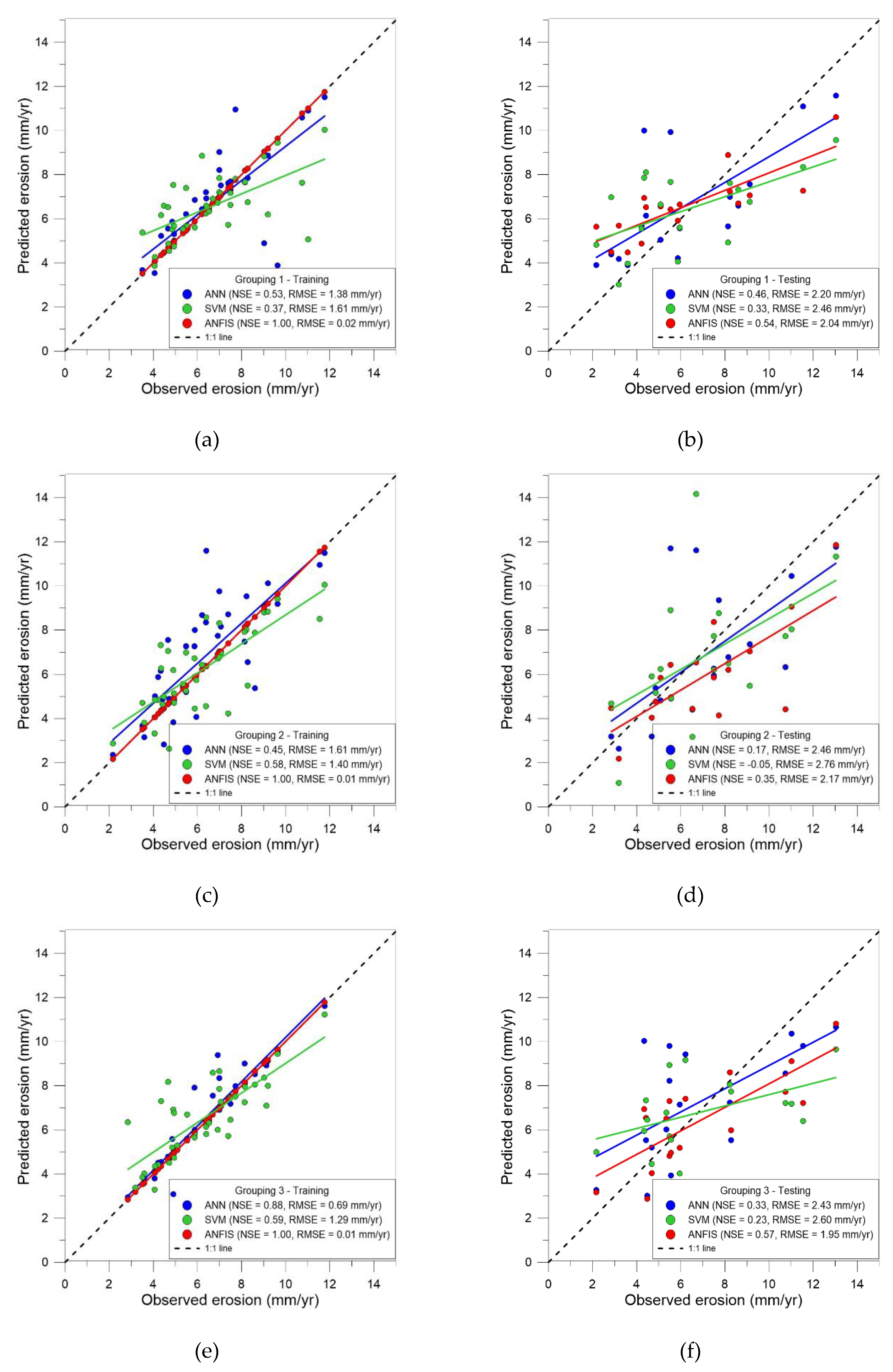
The data in Table 1 provide convincing evidence that ANFIS is the best performing model. We further plotted the predicted values versus the observed values with the regression line and the 1:1 line in the scatter plots of Figure 5. The left-side figures show the training datasets, while the right-side figures are the test datasets. Three different sampling results (groupings) are presented in Figure 5. The first row is grouping #1 (5a and 5b). The second row is grouping #2 (5c and 5d). Finally, the bottom-most row is grouping #3 (5e and 5f). Figure 5 shows that during the training stage, ANFIS successfully tunes its parameters to minimize the errors associated with its predictions. Therefore, the regression line of ANFIS (red) almost coincides with the 1:1 line, and it resulted in an average NSE of 1.00. Coincidentally, the regression line of ANN (blue) is also very close to the 1:1 line in all three cases. However, the data points (blue) are much more scattered around the 1:1 line than those of ANFIS (red) are. Therefore, ANN has a much lower average NSE of 0.62.
As for the test data on the right-hand side of Figure 5, all three models showed substantially more scatter than that of the training data, which indicates substantially bigger errors between the predictions and the observations. The regression line of ANFIS is no longer the closest to the 1:1 line. However, the ANFIS model still has the highest average NSE (0.49) and the lowest average RMSE (2.05 mm/yr). It appears that ANFIS gained its performance advantage due to its hybrid learning approach of combining the ANN and the Fuzzy Inference System.
3.3. Results of Wilcoxon Signed-Rank Test
This study was undertaken to determine the best ML model using NSE, RMSE, and MAE. To determine if the differences between different model predictions were statistically significant, we used the Wilcoxon signed-rank test to compare the errors between different models. With the absolute error of each model being EANFIS, EANN, and ESVM, respectively, the results of the Wilcoxon signed-rank test on the training data for each combination of the three models are summarized in Table 2. The results of the test data were shown in Table 3.
It can be seen from Table 2 that for the training data, the p-values between ANFIS and ANN are all very small and less than the threshold value of 0.05. The same can be said for the p-values between ANFIS and SVM. Taken together, the data presented here provide evidence that ANFIS was a statistically better model than both ANN and SVM when the models were trained with the training data. By contrast, the p-values between ANN and SVM are not small enough to reject the null hypothesis. Therefore, it is inconclusive whether a statistical difference exists in the predictive performance between the two models.
In terms of the test data, however, no statistically significant difference exists between the three models. As shown in Table 3, the p-values are all higher than the threshold value of 0.05. Therefore, we cannot reject the null hypothesis in favor of the alternative hypothesis.
3.4. Comparison with Other ML Algorithms
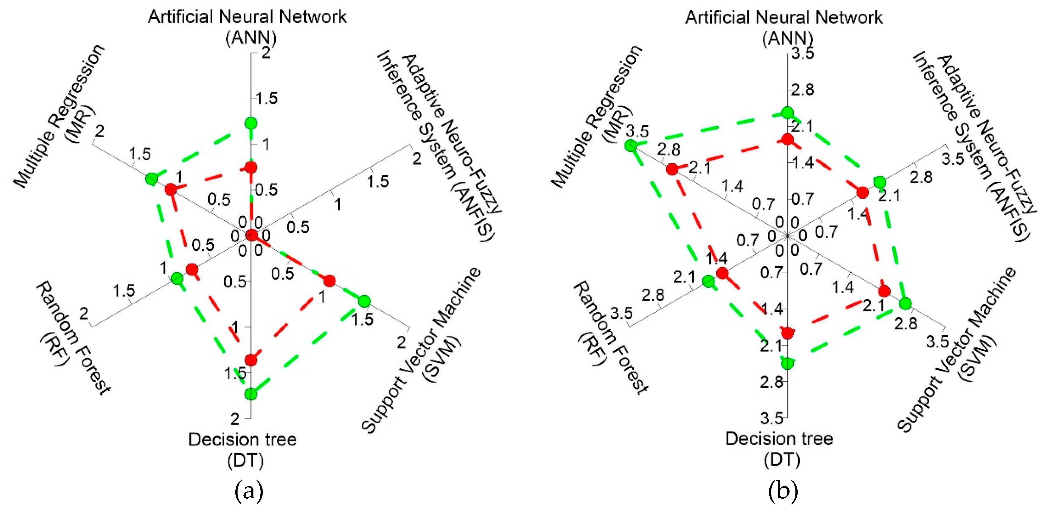
In our previous research, DT, RF, and MR were used to predict the depths of erosion at the Shihmen reservoir watershed study site [27]. The result showed that RF outperforms other ML algorithms. In this study, we further compared the performance of ANN, ANFIS, and SVM to predict soil erosion depths (rates). The results of the above six models are shown together in Figure 6.
Figure 6 shows the comparison between six ML models in terms of the average RMSE (green points) and the average MAE (red points). The sub-Figure 6(a) is based on the training data, and 6(b) is based on the test data. If the points are closer to the center of the radar web, the model will have a better predictive performance. It can be seen from Figure 6a that in terms of RMSE starting from the best to the worst, the six models can be ranked as follows: ANFIS (0.01 mm/yr) < RF (0.93 mm/yr) < ANN (1.23 mm/yr) < MR (1.25 mm/yr) < SVM (1.43 mm/yr) < DT (1.73 mm/yr). It is obvious that ANFIS is the best model for training data. However, because models can perform very well during training but perform poorly in the testing against new data (over-fitted), it is the results of test data that distinguish a good model from a poor one. To evaluate model performance, we should focus on the metrics of test data. It can be seen from Figure 6 that although ANFIS is the best model among the three ML models compared in this study, it is still not quite as good as RF in the previous study. If we rank the six ML models again using the average RMSE of the test data, we will obtain a different rank (starting from the best to the worst): RF (1.75 mm/yr) < ANFIS (2.05 mm/yr) < ANN (2.36 mm/yr) < DT (2.45 mm/yr) < SVM (2.61 mm/yr) < MR (3.47 mm/yr). In other words, RF replaces ANFIS and becomes the favored choice. It is also possible to draw similar conclusions from the MAE values, also in Figure 6.
The results of test data are critical and are emphasized because evaluating the predictive performance of models by training data could lead to over-optimistic and overfitting models. As a result, although ANFIS performs better in training, RF is still considered the best model for predicting the soil erosion rate in the study area. Hannan et al. [45] and Barenboim et al. [46] also compared the performance of RF and ANFIS in their studies. Both studies indicated that the ANFIS and RF models were effective; however, Hannan et al. [45] preferred RF to ANFIS and ANN, and Barenboim et al. [46] recommended both RF and ANFIS.
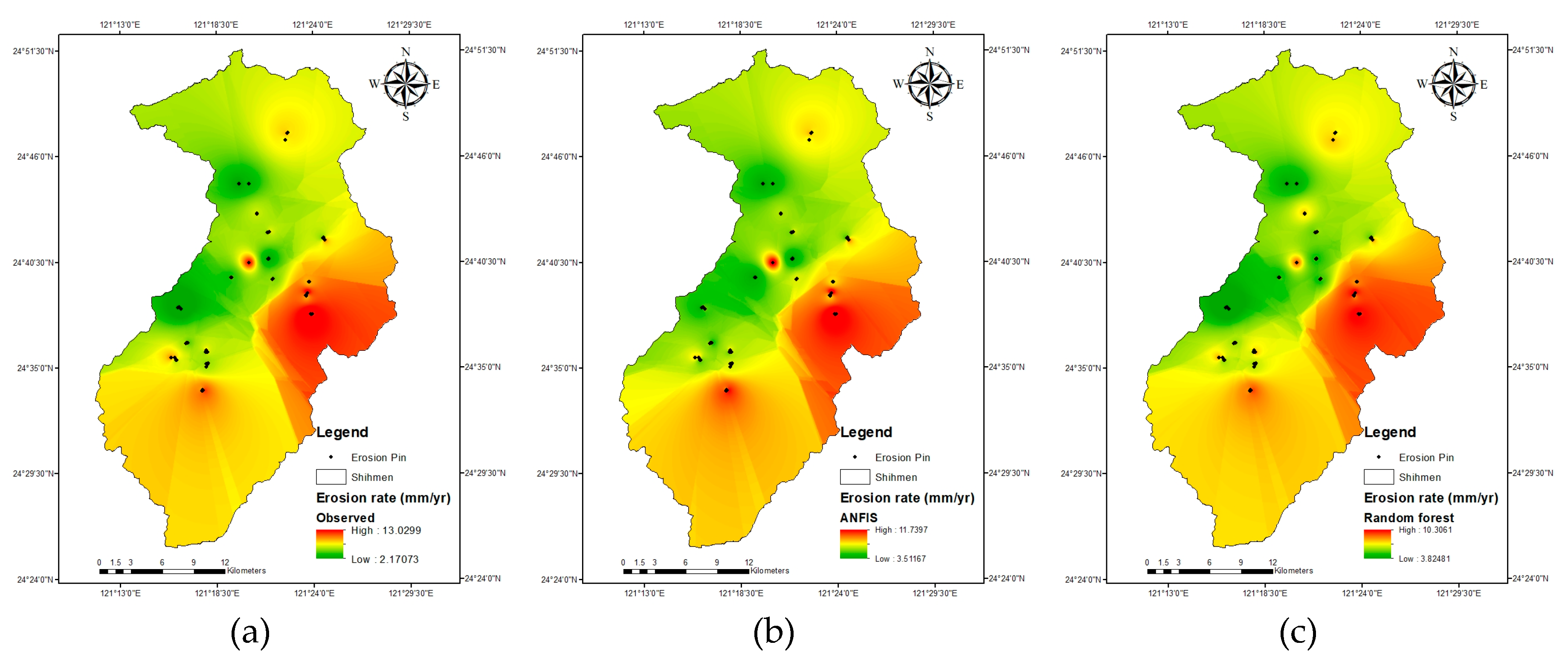
Figure 7 shows the interpolated distribution of erosion rates (mm/yr) in the study watershed using the Inverse Distance Weighting (IDW) method. Figure 7a was obtained from erosion pin measurements, whereas Figure 7b,c were predicted by ANFIS and RF, respectively. It can be seen from the figures that the same distribution pattern is observed. The erosion rate is the highest on the east side of the study area, the lowest on the west side, and the north and south sides have an in-between erosion rate.
4. Conclusions
In this study, the ANN, ANFIS, and SVM algorithms were used to create predictive models of soil erosion rates in the study area of the Shihmen reservoir. The soil erosion rates were measured by 550 erosion pins installed on 55 slopes, and the results of the measurements reflect the sheet and rill erosion that took place within the study area. After dividing the dataset by a 70/30 ratio into training and test datasets using stratified random sampling, ANN, ANFIS, and SVM were used to generate respective models based on the 14 types of factors included in the training data. Then the models were applied to the test data, and the discrepancies from the real measurements were evaluated by R2, NSE, RMSE, and MAE.
Without making an ex-ante choice of soil erosion model, the ex-post outcomes of ML models were quite satisfactory. The average RMSE of the training data ranges from mere 0.01 to 1.43 mm/yr. Among the three models, the performance of ANFIS is considerably higher than those of ANN and SVM, as indicated by its RMSE of 0.01 mm/yr. However, the performance of all three models degraded when they are applied to the test data. Results showed that the average RMSE of the test data varies from 2.05 to 2.61 mm/yr, with ANFIS still the best among the three models. To examine if the difference in prediction is statistically significant, the Wilcoxon signed-rank test was used to conduct pairwise comparisons of the three models. The results indicate that the ANFIS model is better than both the ANN and SVM models for the training data. However, no statistically significant difference exists between the three models when the models are applied to test data.
Moreover, the advantage of ANFIS disappeared when it was compared with the ML models (DT, RF, and MR) developed in our previous study. Although the average RMSE of ANFIS on training data is still unmatched, the average RMSE of ANFIS on test data was worse than that of RF. This shows that ANFIS may have been over-trained, and RF is still considered the best model for predicting the soil erosion rate in the study area.
In this and previous studies, we have made a substantial effort and progress in applying ML algorithms to the prediction of soil erosion rates without resorting to any soil erosion models. Although the effort was made, there is still no shortage of ML algorithms that promise better results than what has been obtained to date. It remains to be seen if ML algorithms are truly viable alternatives to traditional soil erosion models. Future research will have to address this issue in more detail.
Finally, because of the easy installation and wide availability of erosion pins, we believe that the approach presented here is generally applicable to other regions of the world. It would be desirable to obtain such measurements and carry out similar analyses for comparison.
Author Contributions
Conceptualization, W.C.; Data curation, K.A.N. and B.-S.L.; Formal analysis, K.A.N.; Funding acquisition, W.C.; Investigation, B.-S.L.; Methodology, W.C.; Project administration, W.C.; Software, K.A.N.; Supervision, W.C. and U.S.; Writing—original draft, K.A.N.; Writing—review and editing, W.C., B.-S.L. and U.S. All authors have read and agreed to the published version of the manuscript
Funding
This study was partially supported by the National Taipei University of Technology-King Mongkut’s Institute of Technology Ladkrabang Joint Research Program (grant number NTUT-KMITL-108-01) and the Ministry of Science and Technology (Taiwan) Research Project (grant number MOST 108-2621-M-027-001).
Acknowledgments
We thank Kent Thomas for proofreading an early draft of this manuscript. We also thank the anonymous reviewers for their careful reading of our manuscript and insightful suggestions to improve the paper.
Conflicts of Interest
The authors declare no conflict of interests.
References
- Jose, J.; District, P.C.C.; Roosevelt, F.D. Erosion and Sedimentation; University of Connecticut: Haddam, UK, 1993. [Google Scholar]
- Zeneli, G.; Loca, S.; Diku, A.; Lila, A. On-Site and Off-Site Effects of Land Degradation in Albania. Ecopersia 2017, 5, 1787–1797. [Google Scholar]
- Hagans, D.K.; Weaver, W.E.; Madej, M.A. Long-Term on-Site and off-Site Effects of Logging and Erosion in the Redwood Creek Basin, Northern California; Paper Presented at the American Geophysical Union Meeting on Cumulative Effects; Technical Bulletin; National Council of the Paper Industry for Air and Stream Improvement: New York, NY, USA, 1986. [Google Scholar]
- Chen, Z.-S. Establishment of Potential Soil Erosion Map in Western Taiwan and Its Best Management Strategies; Paper presented at the Asia-EC JRC Joint Conference 2017 on “All That Soil Erosion the Global Task to Conserve Our Soil Resource”; Research Center of Surface Soil Resources Inventory and Integration (SSORii): Seoul, South Korea, 2017. [Google Scholar]
- Lin, B.-S.; Chen, C.-K.; Thomas, K.; Hsu, C.-K.; Ho, H.-C. Improvement of the K-Factor of USLE and Soil Erosion Estimation in Shihmen Reservoir Watershed. Sustainability 2019, 11, 355. [Google Scholar] [CrossRef] [Green Version]
- Lo, K.F.A. Quantifying soil erosion for the Shihmen reservoir watershed, Taiwan. Agric. Syst. 1994, 45, 105–116. [Google Scholar] [CrossRef]
- Chen, W.; Li, D.-H.; Yang, K.-J.; Tsai, F.; Seeboonruang, U. Identifying and comparing relatively high soil erosion sites with four DEMs. Ecol. Eng. 2018, 120, 449–463. [Google Scholar] [CrossRef]
- Chiu, Y.J.; Chang, K.T.; Chen, Y.C.; Chao, J.H.; Lee, H.Y. Estimation of soil erosion rates in a subtropical mountain watershed using 137 Cs radionuclide. Nat. Hazards 2011, 59, 271–284. [Google Scholar] [CrossRef]
- Liu, Y.-H.; Li, D.-H.; Chen, W.; Lin, B.-S.; Seeboonruang, U.; Tsai, F. Soil erosion modeling and comparison using slope units and grid cells in Shihmen reservoir watershed in northern Taiwan. Water 2018, 10, 1387. [Google Scholar] [CrossRef] [Green Version]
- Sirvent, J.; Desir, G.; Gutierrez, M.; Sancho, C.; Benito, G. Erosion rates in badland areas recorded by collectors, erosion pins and profilometer techniques (Ebro Basin, NE-Spain). Geomorphology 1997, 18, 61–75. [Google Scholar] [CrossRef]
- Edeso, J.; Merino, A.; Gonzalez, M.; Marauri, P. Soil erosion under different harvesting managements in steep forestlands from northern Spain. Land Degrad. Dev. 1999, 10, 79–88. [Google Scholar] [CrossRef]
- Lin, B.; Thomas, K.; Chen, C.; Ho, H. Evaluation of soil erosion risk for watershed management in Shenmu watershed, central Taiwan using USLE model parameters. Paddy Water Environ. 2016, 14, 19–43. [Google Scholar] [CrossRef]
- Pradhan, B.; Lee, S. Landslide susceptibility assessment and factor effect analysis: Backpropagation artificial neural networks and their comparison with frequency ratio and bivariate logistic regression modelling. Environ. Model. Softw. 2010, 25, 747–759. [Google Scholar] [CrossRef]
- Jang, J.-S. ANFIS: Adaptive-network-based fuzzy inference system. IEEE Trans. Syst. ManCybern. 1993, 23, 665–685. [Google Scholar] [CrossRef]
- Mokhtarzad, M.; Eskandari, F.; Vanjani, N.J.; Arabasadi, A. Drought forecasting by ANN, ANFIS, and SVM and comparison of the models. Environ. Earth Sci. 2017, 76, 729. [Google Scholar] [CrossRef]
- Quej, V.H.; Almorox, J.; Arnaldo, J.A.; Saito, L. ANFIS, SVM and ANN soft-computing techniques to estimate daily global solar radiation in a warm sub-humid environment. J. Atmos. Sol. Terr. Phys. 2017, 155, 62–70. [Google Scholar] [CrossRef] [Green Version]
- Zhou, T.; Wang, F.; Yang, Z. Comparative analysis of ANN and SVM models combined with wavelet preprocess for groundwater depth prediction. Water 2017, 9, 781. [Google Scholar] [CrossRef] [Green Version]
- Angelaki, A.; Singh Nain, S.; Singh, V.; Sihag, P. Estimation of models for cumulative infiltration of soil using machine learning methods. ISH J. Hydraul. Eng. 2018, 1–8. [Google Scholar] [CrossRef]
- Sousa, A.A.R.; Barandica, J.M.; Rescia, A. Ecological and economic sustainability in olive groves with different irrigation management and levels of erosion: A case study. Sustainability (Switzerland) 2019, 11, 4681. [Google Scholar] [CrossRef] [Green Version]
- Abdelwahab, O.M.M.; Ricci, G.F.; De Girolamo, A.M.; Gentile, F. Modelling soil erosion in a Mediterranean watershed: Comparison between SWAT and AnnAGNPS models. Environ. Res. 2018, 166, 363–376. [Google Scholar] [CrossRef]
- Panagopoulos, Y.; Dimitriou, E.; Skoulikidis, N. Vulnerability of a northeast Mediterranean island to soil loss. Can grazing management mitigate erosion? Water (Switzerland) 2019, 11, 1491. [Google Scholar] [CrossRef] [Green Version]
- Srivastava, A.; Brooks, E.S.; Dobre, M.; Elliot, W.J.; Wu, J.Q.; Flanagan, D.C.; Gravelle, J.A.; Link, T.E. Modeling forest management effects on water and sediment yield from nested, paired watersheds in the interior Pacific Northwest, USA using WEPP. Sci. Total Environ. 2020, 701, 134877. [Google Scholar] [CrossRef]
- Kinnell, P.I.A.; Wang, J.; Zheng, F. Comparison of the abilities of WEPP and the USLE-M to predict event soil loss on steep loessal slopes in China. Catena 2018, 171, 99–106. [Google Scholar] [CrossRef]
- Krasa, J.; Dostal, T.; Jachymova, B.; Bauer, M.; Devaty, J. Soil erosion as a source of sediment and phosphorus in rivers and reservoirs – Watershed analyses using WaTEM/SEDEM. Environ. Res. 2019, 171, 470–483. [Google Scholar] [CrossRef] [PubMed]
- Liu, Y.; Fu, B. Assessing sedimentological connectivity using WATEM/SEDEM model in a hilly and gully watershed of the Loess Plateau. Ecol. Indic. 2016, 66, 259–268. [Google Scholar] [CrossRef]
- Morgan, R.; Quinton, J.; Smith, R.; Govers, G.; Poesen, J.; Auerswald, K.; Chisci, G.; Torri, D.; Styczen, M. The European Soil Erosion Model (EUROSEM): A dynamic approach for predicting sediment transport from fields and small catchments. Earth Surf. Process. Landf. J. Br. Geomorphol. Res. Group 1998, 23, 527–544. [Google Scholar] [CrossRef]
- Nguyen, K.A.; Chen, W.; Lin, B.S.; Seeboonruang, U.; Thomas, K. Predicting Sheet and Rill Erosion of Shihmen Reservoir Watershed in Taiwan Using Machine Learning. Sustainability 2019, 11, 3615. [Google Scholar] [CrossRef] [Green Version]
- Tsai, F.; Lai, J.-S.; Chen, W.W.; Lin, T.-H. Analysis of topographic and vegetative factors with data mining for landslide verification. Ecol. Eng. 2013, 61, 669–677. [Google Scholar] [CrossRef]
- Chen, W.; Panahi, M.; Pourghasemi, H.R. Performance evaluation of GIS-based new ensemble data mining techniques of adaptive neuro-fuzzy inference system (ANFIS) with genetic algorithm (GA), differential evolution (DE), and particle swarm optimization (PSO) for landslide spatial modelling. Catena 2017, 157, 310–324. [Google Scholar] [CrossRef]
- Hong, H.; Panahi, M.; Shirzadi, A.; Ma, T.; Liu, J.; Zhu, A.X.; Kazakis, N. Flood susceptibility assessment in Hengfeng area coupling adaptive neuro-fuzzy inference system with genetic algorithm and differential evolution. Sci. Total Environ. 2018, 621, 1124–1141. [Google Scholar] [CrossRef]
- Lee, S.; Kim, Y.-S.; Oh, H.-J. Application of a weights-of-evidence method and GIS to regional groundwater productivity potential mapping. J. Environ. Manag. 2012, 96, 91–105. [Google Scholar] [CrossRef]
- Riaz, M.T.; Basharat, M.; Hameed, N.; Shafique, M.; Luo, J. A Data-Driven Approach to Landslide-Susceptibility Mapping in Mountainous Terrain: Case Study from the Northwest Himalayas, Pakistan. Nat. Hazards Rev. 2018, 19, 05018007. [Google Scholar] [CrossRef]
- Chen, W.; Chen, A. A Statistical Test of Erosion Pin Measurements; Paper Presented at the 39th Asian Conference on Remote Sensing (ACRS 2018); Asian Association of Remote Sensing (AARS): Kuala Lumpur, Malaysia, 2018. [Google Scholar]
- Lee, S.; Ryu, J.-H.; Lee, M.-J.; Won, J.-S. Use of an artificial neural network for analysis of the susceptibility to landslides at Boun, Korea. Environ. Geol. 2003, 44, 820–833. [Google Scholar] [CrossRef]
- Hecht-Nielsen, R. Kolmogorov’s mapping neural network existence theorem. In Proceedings of the International Conference on Neural Networks; IEEE Press: New York, NY, USA, 1987; Volume 3. [Google Scholar]
- Schölkopf, B.; Burges, C.J.; Smola, A.J. Advances in Kernel Methods: Support Vector Learning; MIT Press: Cambridge, MA, USA, 1999. [Google Scholar]
- Despotovic, M.; Nedic, V.; Despotovic, D.; Cvetanovic, S. Evaluation of empirical models for predicting monthly mean horizontal diffuse solar radiation. Renew. Sustain. Energy Rev. 2016, 56, 246–260. [Google Scholar] [CrossRef]
- Moriasi, D.N.; Arnold, J.G.; Van Liew, M.W.; Bingner, R.L.; Harmel, R.D.; Veith, T.L. Model evaluation guidelines for systematic quantification of accuracy in watershed simulations. Trans. ASABE 2007, 50, 885–900. [Google Scholar] [CrossRef]
- Verstraeten, G.; Prosser, I.P.; Fogarty, P. Predicting the spatial patterns of hillslope sediment delivery to river channels in the Murrumbidgee catchment, Australia. J. Hydrol. 2007, 334, 440–454. [Google Scholar] [CrossRef]
- Gupta, S.K.; Goyal, M.R. Soil Salinity Management in Agriculture: Technological Advances and Applications; Apple Academic Press Inc.: Waretown, NJ, USA, 2017. [Google Scholar]
- Willmott, C.J.; Matsuura, K. Advantages of the mean absolute error (MAE) over the root mean square error (RMSE) in assessing average model performance. Clim. Res. 2005, 30, 79–82. [Google Scholar] [CrossRef]
- Teke, A.; Yıldırım, H.B.; Çelik, Ö. Evaluation and performance comparison of different models for the estimation of solar radiation. Renew. Sustain. Energy Rev. 2015, 50, 1097–1107. [Google Scholar] [CrossRef]
- Nash, J.E.; Sutcliffe, J.V. River flow forecasting through conceptual models part I—A discussion of principles. J. Hydrol. 1970, 10, 282–290. [Google Scholar] [CrossRef]
- Krause, P.; Boyle, D.; Bäse, F. Comparison of different efficiency criteria for hydrological model assessment. Adv. Geosci. 2005, 5, 89–97. [Google Scholar] [CrossRef] [Green Version]
- Hannan, M.; Ali, J.A.; Mohamed, A.; Uddin, M.N. A random forest regression based space vector PWM inverter controller for the induction motor drive. IEEE Trans. Ind. Electron. 2017, 64, 2689–2699. [Google Scholar] [CrossRef]
- Barenboim, M.; Masso, M.; Vaisman, I.I.; Jamison, D.C. Statistical geometry based prediction of nonsynonymous SNP functional effects using random forest and neuro-fuzzy classifiers. Proteins Struct. Funct. Bioinform. 2008, 71, 1930–1939. [Google Scholar] [CrossRef]
Figure 1.
The study area is Northern Taiwan’s Shihmen reservoir.

Figure 2.
The research framework of this study.

Figure 3.
The model of ANN used in this study.

Figure 4.
Illustration of the symbols used in the Equations (2)–(5).

Figure 5.
X-Y plots of predicted values vs. observed values: (a) Grouping #1—Training data; (b) Grouping #1—Test data; (c) Grouping #2—Training data; (d) Grouping #2—Test data; (e) Grouping #3—Training data; (f) Grouping #3—Test data.
Figure 5.
X-Y plots of predicted values vs. observed values: (a) Grouping #1—Training data; (b) Grouping #1—Test data; (c) Grouping #2—Training data; (d) Grouping #2—Test data; (e) Grouping #3—Training data; (f) Grouping #3—Test data.

Figure 6.
Radar plots of six ML models: (a) Training data; (b) Test data.

Figure 7.
Distribution of erosion rates in the study area: (a) Observed; (b) Predicted by ANFIS; (c) Predicted by RF.
Figure 7.
Distribution of erosion rates in the study area: (a) Observed; (b) Predicted by ANFIS; (c) Predicted by RF.


Table 1.
The performance metrics of the ANFIS, ANN, and SVM models.
| ANN | ANFIS | SVM | |||||
|---|---|---|---|---|---|---|---|
| Train | Test | Train | Test | Train | Test | ||
| Grouping #1 | R2 | 0.59 | 0.49 | 1.00 | 0.66 | 0.37 | 0.33 |
| NSE | 0.53 | 0.46 | 1.00 | 0.54 | 0.37 | 0.33 | |
| RMSE (mm/yr) | 1.38 | 2.20 | 0.02 | 2.04 | 1.60 | 2.46 | |
| MAE (mm/yr) | 0.71 | 1.71 | 0.01 | 1.73 | 1.03 | 2.11 | |
| Grouping #2 | R2 | 0.62 | 0.40 | 1.00 | 0.54 | 0.59 | 0.28 |
| NSE | 0.45 | 0.17 | 1.00 | 0.35 | 0.58 | -0.05 | |
| RMSE (mm/yr) | 1.61 | 2.46 | 0.01 | 2.17 | 1.40 | 2.76 | |
| MAE (mm/yr) | 1.18 | 1.81 | 0.01 | 1.61 | 1.03 | 2.18 | |
| Grouping #3 | R2 | 0.90 | 0.39 | 1.00 | 0.60 | 0.61 | 0.24 |
| NSE | 0.88 | 0.33 | 1.00 | 0.57 | 0.59 | 0.23 | |
| RMSE (mm/yr) | 0.69 | 2.43 | 0.01 | 1.95 | 1.29 | 2.60 | |
| MAE (mm/yr) | 0.36 | 2.02 | 0.01 | 1.67 | 0.90 | 2.13 | |
| Average | R2 | 0.70 | 0.43 | 1.00 | 0.60 | 0.52 | 0.28 |
| NSE | 0.62 | 0.32 | 1.00 | 0.49 | 0.51 | 0.17 | |
| RMSE (mm/yr) | 1.23 | 2.36 | 0.01 | 2.05 | 1.43 | 2.61 | |
| MAE (mm/yr) | 0.75 | 1.85 | 0.01 | 1.67 | 0.99 | 2.14 | |
Table 2.
The results of the Wilcoxon signed-rank test (training data).
| P-value (Training) | ANFIS-ANN | ANFIS-SVM | ANN-SVM |
|---|---|---|---|
| Ho: Null hypothesis Ha: Alternative hypothesis | Ho: EANFIS = EANN Ha: EANFIS < EANN | Ho: EANFIS = ESVM Ha: EANFIS < ESVM | Ho: EANN = ESVM Ha: EANN < ESVM |
| Grouping #1 | < 0.001 | < 0.001 | 0.046 |
| Grouping #2 | < 0.001 | < 0.001 | 0.777 |
| Grouping #3 | < 0.001 | < 0.001 | < 0.001 |
Table 3.
The results of the Wilcoxon signed-rank test (test data).
| P-value (Test) | ANFIS-ANN | ANFIS-SVM | ANN-SVM |
|---|---|---|---|
| Ho: Null hypothesis Ha: Alternative hypothesis | Ho: EANFIS = EANN Ha: EANFIS < EANN | Ho: EANFIS = ESVM Ha: EANFIS < ESVM | Ho: EANN = ESVM Ha: EANN < ESVM |
| Grouping #1 | 0.6267 | 0.1317 | 0.1530 |
| Grouping #2 | 0.6944 | 0.1030 | 0.1421 |
| Grouping #3 | 0.2293 | 0.0540 | 0.3221 |
© 2020 by the authors. Licensee MDPI, Basel, Switzerland. This article is an open access article distributed under the terms and conditions of the Creative Commons Attribution (CC BY) license (http://creativecommons.org/licenses/by/4.0/).
Share and Cite
MDPI and ACS Style
Nguyen, K.A.; Chen, W.; Lin, B.-S.; Seeboonruang, U. Using Machine Learning-Based Algorithms to Analyze Erosion Rates of a Watershed in Northern Taiwan. Sustainability 2020, 12, 2022. https://doi.org/10.3390/su12052022
AMA Style
Nguyen KA, Chen W, Lin B-S, Seeboonruang U. Using Machine Learning-Based Algorithms to Analyze Erosion Rates of a Watershed in Northern Taiwan. Sustainability. 2020; 12(5):2022. https://doi.org/10.3390/su12052022
Chicago/Turabian StyleNguyen, Kieu Anh, Walter Chen, Bor-Shiun Lin, and Uma Seeboonruang. 2020. "Using Machine Learning-Based Algorithms to Analyze Erosion Rates of a Watershed in Northern Taiwan" Sustainability 12, no. 5: 2022. https://doi.org/10.3390/su12052022
Note that from the first issue of 2016, this journal uses article numbers instead of page numbers. See further details here.