Article

Examining Hybrid and Single SVM Models with Different Kernels to Predict Rock Brittleness

by
Danial Jahed Armaghani
1,
Panagiotis G. Asteris
2,*,
Behnam Askarian
3,
Mahdi Hasanipanah
4,*,
Reza Tarinejad
5 and
Van Van Huynh
1
1
Modeling Evolutionary Algorithms Simulation and Artificial Intelligence, Faculty of Electrical & Electronics Engineering, Ton Duc Thang University, Ho Chi Minh City 758307, Vietnam
2
Computational Mechanics Laboratory, School of Pedagogical and Technological Education, 14121 Heraklion, Athens, Greece
3
Department of Electrical and Computer Engineering, Texas Tech University, Lubbock, TX 79409, USA
4
Institute of Research and Development, Duy Tan University, Da Nang 550000, Vietnam
5
Department of Civil Engineering, University of Tabriz, 29 Bahman Blvd, Tabriz 51666, Iran
*
Authors to whom correspondence should be addressed.
Sustainability 2020, 12(6), 2229; https://doi.org/10.3390/su12062229
Submission received: 10 February 2020 / Revised: 8 March 2020 / Accepted: 10 March 2020 / Published: 12 March 2020

Abstract

:
The aim of this study was twofold: (1) to assess the performance accuracy of support vector machine (SVM) models with different kernels to predict rock brittleness and (2) compare the inputs’ importance in different SVM models. To this end, the authors developed eight SVM models with different kernel types, i.e., the radial basis function (RBF), the linear (LIN), the sigmoid (SIG), and the polynomial (POL). Four of these models were developed using only the SVM method, while the four other models were hybridized with a feature selection (FS) technique. The performance of each model was assessed using five performance indices and a simple ranking system. The results of this study show that the SVM models developed using the RBF kernel achieved the highest ranking values among single and hybrid models. Concerning the importance of variables for predicting the brittleness index (BI), the Schmidt hammer rebound number (Rn) was identified as the most important variable by the three single-based models, developed by POL, SIG, and LIN kernels. However, the single SVM model developed by RBF identified density as the most important input variable. Concerning the hybrid SVM models, three models that were developed using the RBF, POL, and SIG kernels identified the point load strength index as the most important input, while the model developed using the LIN identified the Rn as the most important input. All four single-based SVM models identified the p-wave velocity (Vp) as the least important input. Concerning the least important factors for predicting the BI of the rock in hybrid-based models, Vp was identified as the least important factor by FS-SVM-POL, FS-SVM-SIG, and FS-SVM-LIN, while the FS-SVM-RBF identified Rn as the least important input.

1. Introduction

In every ground excavation project, the rock brittleness needs to be measured as a key property of rock mass. In designing geotechnical engineering structures, especially those that are constructed on the rock mass, a proper insight into the rock’s brittleness is of great value. For instance, using rock-brittleness-related information, engineers are able to assess the wellbore stability and performance quality of a hydraulic fracturing job [1,2]. In addition, with the use of such information, the shale rocks mechanic properties can be regulated well. Meanwhile, a number of parameters, including the volumetric fraction of strong minerals, carbonates, weak elements, and pores, can be used to define the Young’s modulus and strength of these properties [3,4]. Brittleness also plays an important role in assessing the stability of the surrounding rock mass in deep underground projects [5].
Brittleness can be the reason behind numerous disastrous incidents associated with rock mechanics, such as rock-bursts [6,7,8,9]. According to the literature, in the prediction performance of the tunnel boring machines (TBMs) and roadheaders, brittleness can be taken into account as a significant and effective factor [10,11]. Moreover, this property can effectively define the excavation effectiveness of drilling, which is a parameter of a great effect in coal mining processes [12,13]. As a result, an important part of the projects related to geotechnical and rock engineering, is the measurement of rock brittleness [7]. Despite all facts explained above, Altindag [14] argued that no consensus exists on defining and measuring standards of this brittleness. On the other hand, according to Yagiz [13], various properties of the rock influence rock brittleness. A number of researchers have stated that brittleness is related to the lack of ductility or ductility inversion [15]. Brittleness was defined by Ramsey [16] as the loss of the inter-particle cohesion of a rock. According to Obert and Duvall [17], brittleness is the inclination of a material, like cast iron or lots of rock types, to split due to being subjected to a pressure equivalent to or higher than the yield stress of the material. Normally, highly brittle rock has six characteristics: (1) failure under an insignificant force, (2) having a great compressive-to-tensile strength ratio, (3) the production of small particles, (4) great interior friction angle, (5) great firmness, and (6) the generation of completely developed characteristics following hardness lab experiments [15,17]. A review of literature indicates that most of studies carried out into rock brittleness index (BI) have been on the basis of the relationship between tensile and uniaxial compressive strengths of the rock samples [18,19,20,21,22]. Nevertheless, only a few researchers have discussed a relationship between BI and other rock properties, such as hardness, quartz content, elasticity modulus, internal friction angle, Poisson’s ratio, etc. [23,24,25]. The models presented have not shown enough capability to estimate BI. The reason is that the majority of these models make use of one or two dependent parameters [13,21,22].
In recent years, many researchers have applied soft computing (SC), artificial intelligence (AI), and machine learning (ML) techniques to solve science and engineering problems [8,26,27,28,29,30,31,32,33,34,35,36,37,38,39,40,41,42,43,44,45,46,47,48,49,50,51,52,53,54,55,56,57,58,59,60,61,62,63,64,65,66,67,68,69,70,71,72,73,74,75]. Although a number of researchers have already confirmed the applicability of ML techniques for solving problems appearing in engineering fields, numerous ML techniques have still remained unused in studies focusing on rock BI prediction. A comprehensive review of the literature showed that no study has been published examining the viability of popular ML techniques, e.g., support vector machine (SVM), in the prediction of BI values. Thus, this study aims to assess the feasibility of SVM to predict BI. To this end, eight SVM models are developed with different approaches. In the following, the principles of the methods and the descriptions of the used material are described. Then, after proposing several empirical equations to predict the rock BI, the design process of ML models and their results will be discussed. Eventually, the best ML model is selected and introduced to predict rock BI.

2. Related Works

Several studies proposed empirical formulas to approximate the rock brittleness [24,25,76,77]. The majority of these studies considered the relationship between tensile and uniaxial compressive strength of the rock samples. Hucka and Das [25] proposed two formulas as B1 = σct and B2 = σc − σtc + σt, where σc and σt denote the uniaxial compression strength and tensile strength, respectively. Altindag [78] and Yarali and Soyer [79] developed the following formulas, respectively: B3 = σc * σt/2. B4 = (σc * σt)0.72. Meng et al. [20] and Nejati and Moosavi [24] developed the following formula, respectively, using more factors: B5 = σc0.84 + E0.51t0.21 and B6 = (σp − σc)/sp. In this formula, σc, σt, σp, and E denote the uniaxial compression strength, tensile strength, peak strength, and elastic modulus, respectively. Among these empirical equations, the general form (B1), which was proposed by Hucka and Das [25], is the most commonly used by other researchers [13,21,22]. In the prediction of the rock BI value, the single input and the multi-inputs predictive systems such as simple and multiple linear regression models have used [22,23,24,25]. Although multiple linear regression models demonstrated a higher precision level in comparison with the available simple regression models [18,21,22], they are not always robust enough to describe the behavior of complex systems accurately [62,80]. In addition, the accuracy level of these models is not good enough for prediction of rock BI [21,22].
In field of ML, AI, and SC techniques, only limited research has been carried out for the aim of predicting the BI values of rock. Kaunda and Asbury [81] made use of an artificial neural network (ANN) technique with the help of system inputs like the Poisson’s ratio, unit weight, the velocity of the S and P waves, and the elastic modulus. Forming fuzzy inference system (FIS) and conducting non-linear regression analysis, Yagiz and Gokceoglu [18] attempted to predict rock BI. For the development of these models, the uniaxial compressive strength (UCS), unit weight, and Brazilian tensile strength (BTS) of the rock were used as inputs. Their finding showed that the FIS model can be effectively applied to the same field for further research. Some predictive equations were suggested by Koopialipoor et al. [21] to calculate the BI value of rock as a function of intact rock properties, such as density, p-wave velocity, and the Schmidt hammer rebound number. They hybridized ANN and the firefly algorithm into a single model aiming at developing the proposed equations. In another study, the genetic programming model feasibility was tested by Khandelwal et al. [22] in a way to predict the intact rocks brittleness level. For the purpose of estimating the BI of rock mass, they employed multiple input variables, such as BTS, UCS, and unit weight. As the literature review shows, many soft computing methods, such as SVM, have not been used to predict the BI. Due to this, the authors decided to apply and develop SVM models to predict BI of the rock samples.

3. Methods and Materials

3.1. Support Vector Machine (SVM)

The support vector machine (SVM) is viewed as a supervised ML method that employs statistical learning theory and the structural risk minimization principle [82]. The SVM reformats the non-linear world into the linear by generating a hyperplane and changes it to a simple and processable format [78] (Figure 1). This transformation of data is performed using a mathematical function that is known as the kernel function. The training dataset helps the SVM to transform the inputs into a high-dimensional feature space. In the original space of n coordinates, a separating hyperplane is created between the points of two distinct classes. In fact, the SVM is a linear two-class classifier and aims to find a maximum margin of separation between the classes and constructs a classification hyperplane in the central of the maximum margin [79,83]. The two classes are labelled as +1 (positive examples), which denotes the case that is above the hyperplane, and -1 (negative examples), which represents the case that is below the hyperplane. For predicting the group to which a new record should belong, the features of new data subsequently can be used. The closest training points to the hyperplane are called support vectors. Once the decision surface is attained, the classification of new data can be performed [82].
As pointed out earlier, the margin maximization is viewed as regularizing the solution by minimizing w. This is performed for both classification and regression. For classification, this minimization is performed under the condition that all examples are classified correctly while regression following the condition that the value y of all instances differs lees than the needed accuracy ϵ from f(x) for regression.
In another words, for classification, the main aim is to find a function f(x) = wx + b where f(x) ≥ 1 for positive examples and f(x) ≤ −1 for negative examples. Under these conditions, we want to maximize the margin, which is nothing more than minimizing the derivative of f′ = w. For regression, the aim is to find a function f(x) = wx + b (orange line) following the condition that f(x) is within a required accuracy ϵ from the value y(x) (gray bars) of every data point, i.e., |y(x) − f(x)| ≤ ϵ, where epsilon is the distance between the dashed and the orange line (Figure 2).
In this study, the SVM model with different kernels, i.e., the radial basis function (RBF), the linear (LIN), the sigmoid (SIG), and the polynomial (POL) is investigated to solve the problem. In machine learning, a “kernel” is customarily employed to refer to the kernel trick, a method of adopting a linear classifier to solve a non-linear problem. When a linear separation of the data is straightforward, a LIN kernel function should be used. In other situations, one of the other functions can be used. For some SVM parameters, the SIG functions are very similar to the RBF kernel [84]. The LIN kernel is the specific case of the RBF, and in the cases where RBF is employed in the processing, it is not required to utilize the LIN. Concerning the accuracy, the RBF kernel has a higher capability in interpolation than the SIG, which causes the RBF to yield more reliable results. On the other hands, the RBF kernel is weak in producing longer-range extrapolation. The SIG kernel might have large variance because it is not strictly positive definite that may lead to in-correct approximation. Tehrany, et al. [85] pointed out that the POL kernel is capable of better extrapolation. The kernels’ formulas are presented in Table 1. To examine the efficiency of each kernel to predict the BI, all four types of kernels were used. Multiple important parameters exist that are required to define the kernel types, including Gamma (γ) for RBF, POL, and SIG, while "d" is the term of polynomial degree for the POL kernel.

3.2. Acquisition of Data

The data used in this study was obtained from a tunneling project in Pahang state, Malaysia. This tunnel provides a flow path of freshwater. This tunnel discharges about 27.6 cubic meters per second under free-flow conditions. Other tunnel specifications include tunnel length (44.6 km), diameter (5.2 m), and longitudinal gradient (1/1900). In total, 35 km of the tunnel was excavated with three TBMs and the rest of the tunnel was excavated with the help of a drilling and blasting technique. While most of the rocks excavated with the mentioned techniques were made of granite, the geological units also included metamorphic and some sedimentary rocks. This present study massively investigated the geotechnical aspects of the tunnel to get rock samples for conducting rock index tests. Thus, the research team collected 120 granite block samples from the tunnel face in multiple locations and different tunnel distances and then these block samples were transferred to the rock mechanics laboratory to carry out the tests. To conduct the laboratory tests, the team attempted to collect representative rock blocks that had no deficiency and discontinuities. Then, the block rock samples were prepared based on the suggested procedure by the International Society for Rock Mechanics [86] for each planned test. An experimental program consists of laboratory tests, i.e., the Schmidt hammer, BTS, density, UCS, p-wave, and point load were planned and conducted on the samples. Then, the obtained results were considered for the modeling of this study. The BI values were calculated based on the main suggestion of the literature, which is B I = U C S B T S , and then set as model output. The corresponding model inputs considered were the Schmidt hammer rebound number (Rn), p-wave velocity (Vp), point load strength index (Is50), and density (D). Figure 3 and Figure 4 show the conducted BTS and UCS tests on the samples and their failures, respectively.
Various ranges, i.e., (2870–7702 m/s), (2.37–2.79 g/cm3), (20–61), (0.89-7.1 MPa) and (8.9–24.01) were obtained and considered for Vp, D, Rn, Is50, and BI, respectively. In addition, the average value of each parameter within the database was calculated as 5491.6 m/s, 2.59 g/cm3, 40.5, 3.6 MPa, and 15.5, respectively. It should be noted that 110 datasets were used to develop and train the models presented in this study for rock BI prediction. In the following section, the relationships between the input and output parameters are investigated in detail.

3.3. Correlations between Inputs and Output

This section investigates the relationships between system inputs and output and also between the inputs themselves. The proposed equations to predict the BI of the rock, together with their performance based on coefficient of correlation (R), are shown in Table 2. By proposing these equations, R range of 0.730–0.815 was obtained using model inputs (i.e., Vp, D, Rn, and Is50), which indicates that these inputs are capable to receive a suitable and acceptable predication performance. However, most of the times, a higher level of these performance predictions is of more interest by designers and engineers in real conditions. Therefore, it seems that the use of multi-inputs could add more advantages of BI design in practice. The results of R between the inputs and output and also for the inputs themselves, as well as their scatter plots, are shown in Figure 5. It is obvious that the output is dependent on all inputs, while, furthermore, the inputs also show considerable and significant relations between each other. In light of the above, it can be concluded that the use of all 4 model inputs, i.e., Vp, D, Rn, and Is50 together may increase the performance capacity. This can be done by proposing ML and SC techniques in predicting the BI of the rock samples.

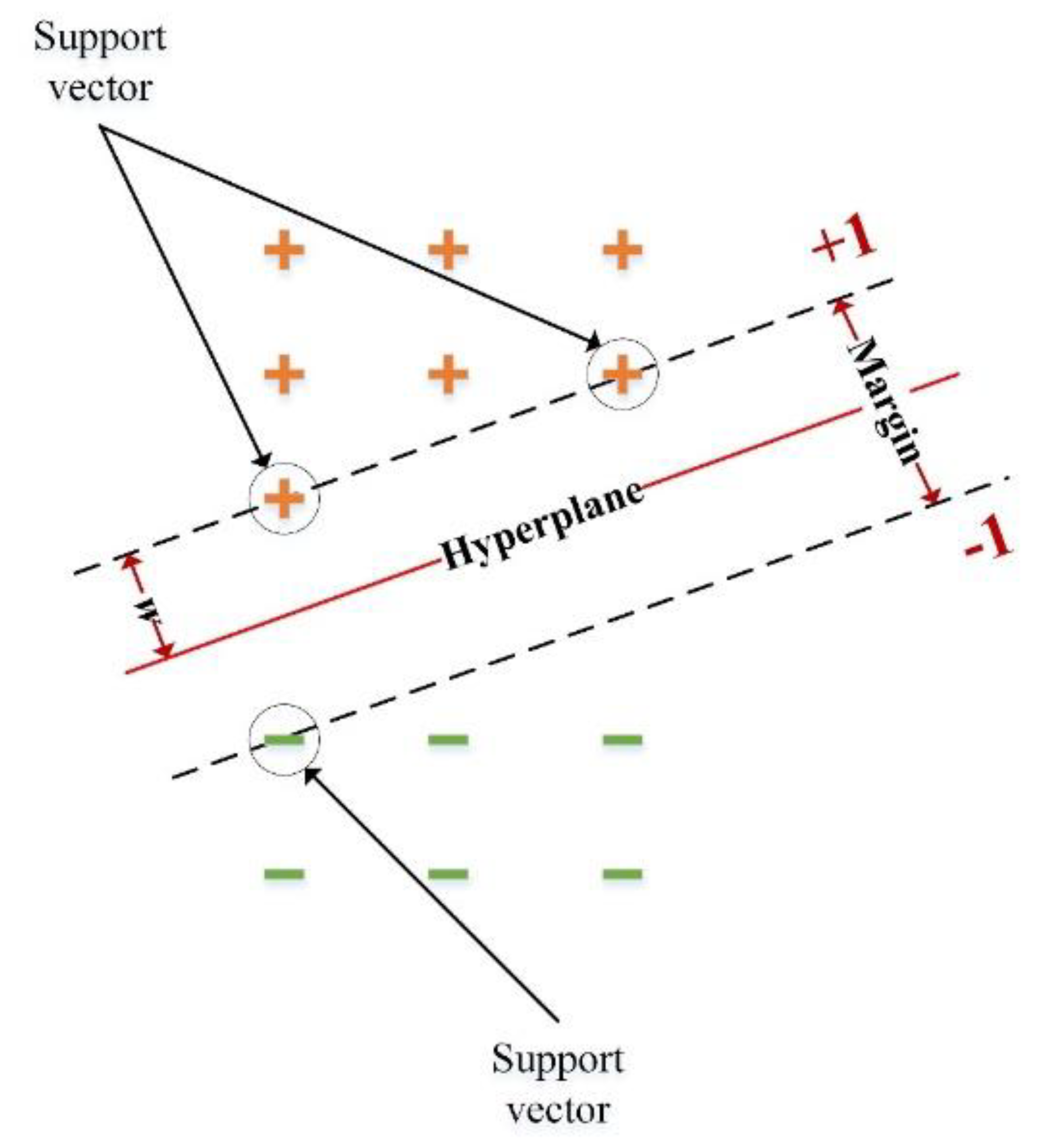
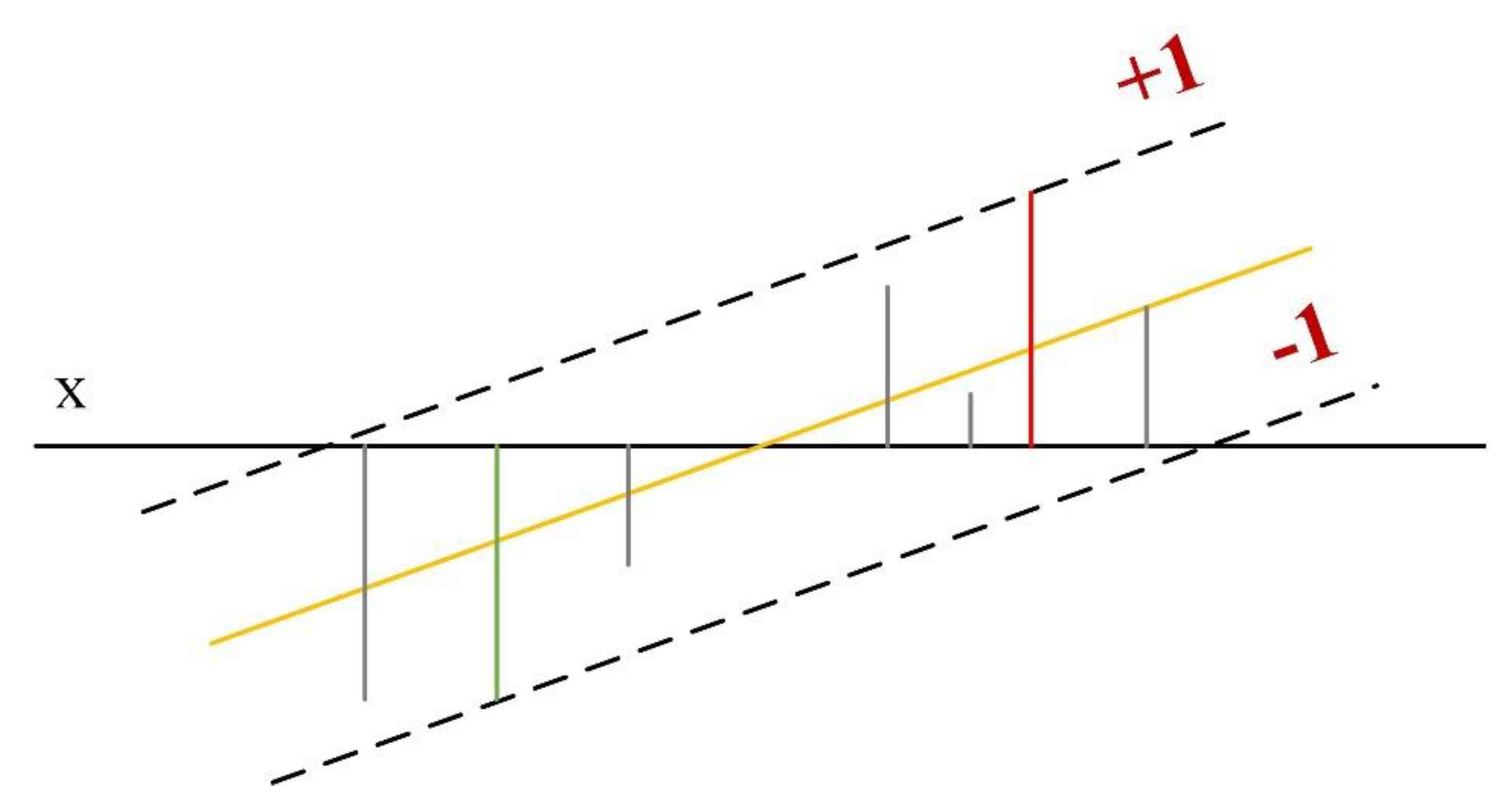
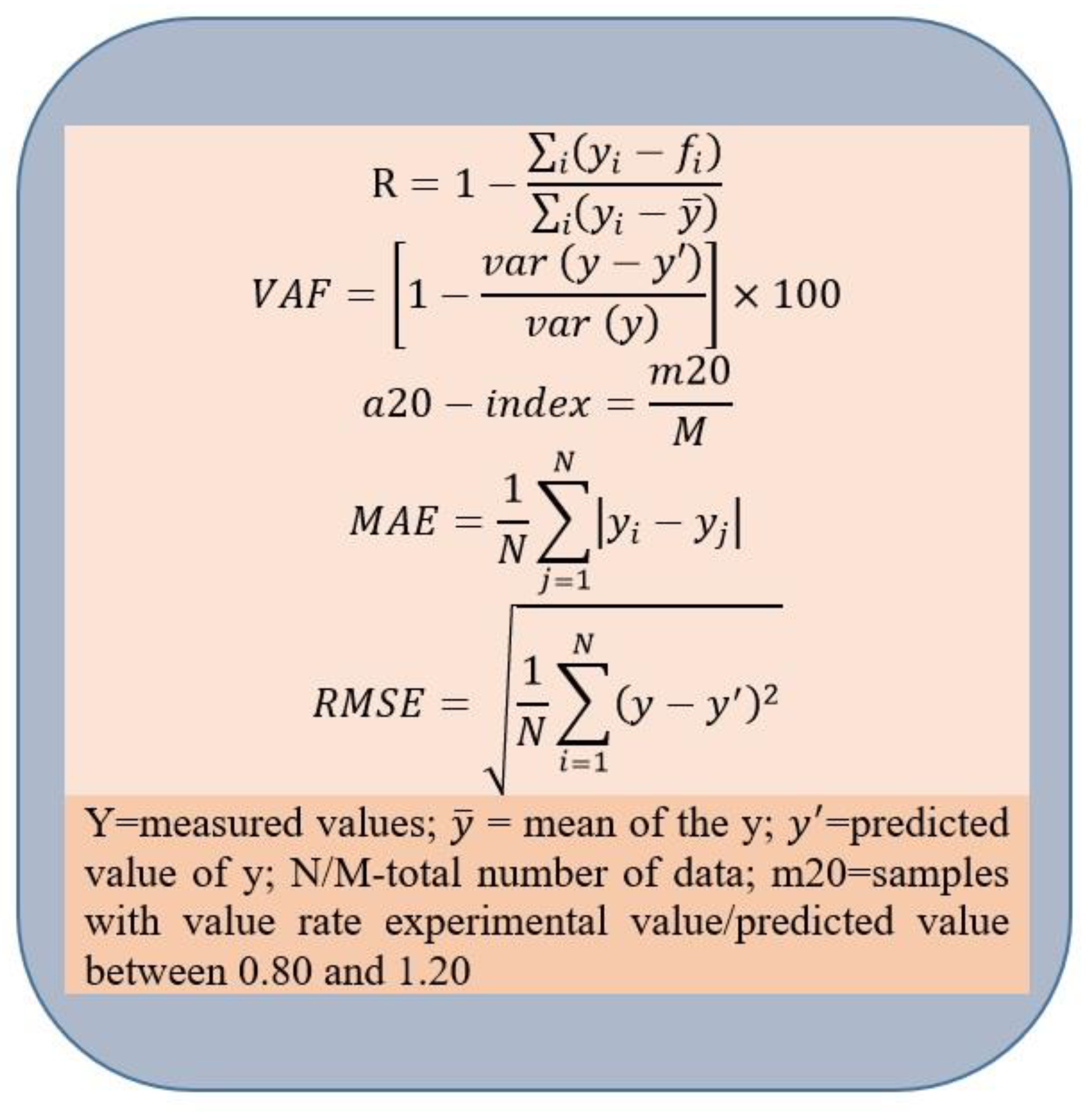
4. Results and Evaluations

This study developed four single and four hybrid SVM models with different kernels to predict rock BI. Thus, four models were single-based and four models were hybrid-based. This study used five performance indices, including R, the root means square error (RMSE), the mean absolute error (MAE), the variance account for (VAF), and the a20-index to evaluate the accuracy performance of these eight models (Figure 6). The research team also used a simple ranking method to rank the performance of the developed models. In this method, each model was evaluated within the training and testing phase separately. For each performance indicator, the highest rank equaled four (4) because each classification included four models. Accordingly, the lowest rank equaled one (1) (if the multiple models do not obtain an equal value for a certain indicator). For the models that achieved the same value for a certain indicator, an equal rank was assigned. For each phase, the sum of the ranks was calculated. Finally, the cumulative ranking was calculated for each model by summing the training and testing ranks. More details regarding the ranking system and its calculation process can be found in the original study conducted by Zorlu et al. [87].
Four single-SVM models were developed using different kernels, including RBF, POL, SIG, and LIN. To develop each of these models, several parameters were identified and employed. These parameters are shown in Table 3. First of all, the authors used a stopping criterion, which stood for determining when to stop the optimization algorithm. To control the trade-off between maximizing the margin and minimizing the training error term, a value of regularization parameter (C) was used. A regression precision (epsilon) value which caused errors to be accepted provided that they are less than the value specified here. RBF gamma was used only for the RBF kernel, while the gamma was used only for the POL and SIG kernels. Both gammas improved the classification accuracy and reduced the regression error for the training data. Finally, the “degree”, controlled the complexity of the mapping space, and was used only for the polynomial kernel.
To develop the hybrid-based models, the research team initially performed an input selection to identify the most relevant inputs and remove the irrelevant data. Thus, a feature selection (FS) technique was used. The FS used the likelihood ratio, which tests for target-input independence. The following criteria to perform the screening were used: (1) the maximum percentage of missing values (70.0) and (2) the minimum coefficient of variation (0.1). The FS was performed using four inputs, including Vp, D, Rn, and Is50. Finally, the FS removed “D” from the list of inputs. Once the FS was performed, the authors again developed the SVM models using different kernels. As previously mentioned, several parameters were used to develop the hybrid-based SVM models that are shown in Table 4.
The performance index results of the single-based models together with their ranking values are presented in Table 5. The results show that the SVM-RBF model achieved the highest rank for both training (19) and testing (17) phases. Consequently, this model achieved the highest cumulative rank (36). This model was followed by SVM-POL, SVM-LIN, and SVM-SIG models, respectively. Concerning the hybrid-based models, the results of which are shown in Table 6, the FS-SVM-RBF model obtained the highest rank for training (20), while the FS-SVM-POL obtained the highest rank for testing (18). In terms of cumulative ranking, the FS-SVM-RBF achieved the highest rank (31).
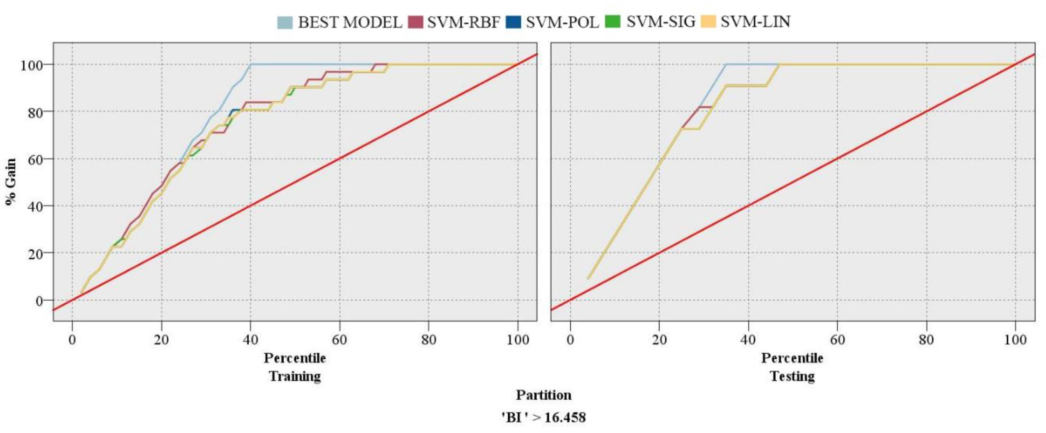
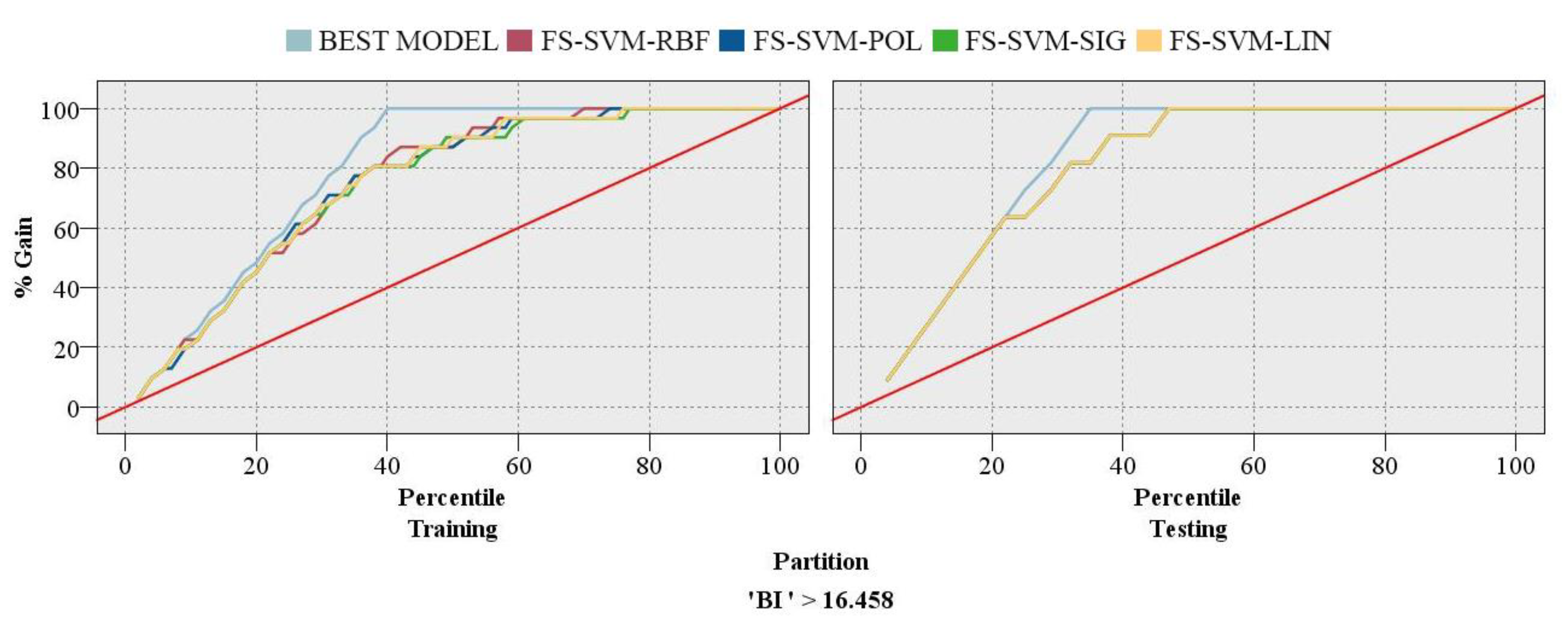
This present study also employed a chart of gains to evaluate the performance of the SVM models that were developed. Gains can be computed as follows:
G a i n s = ( n N ) × 100
where n denotes the number of hits in quantile and N denotes the total number of hits. Here, it is necessary to mention that “hit” refers to the success of a model to predict the values greater than the midpoint of the fields range (BI > 16.458). In the gains chart, the blue line signifies the perfect model that has perfect confidence (where hits = 100% of cases), the diagonal red line represents the at-chance model, and the other lines in the middle represent the other models. To compare a model developed and the at-chance model, the area between a model and the red line can be used. In fact, this area identifies how much better a proposed model is compared to the at-chance model. Moreover, the area between a model proposed and the perfect model identifies where a proposed model can be improved.
In the gains chart, it is necessary to maximize the space between the models’ curves and at-chance model. Moreover, the higher lines show better models, particularly on the left side of the chart. Figure 7 shows the gains chart for single-based SVM models in predicting the rock BI. For the training phase, the SVM-RBF model was the best (the highest line/maximum space between the model curve and the at-chance model) and the SVM-LIN was the worst (the lowest line/minimum space between the model curve and the at-chance model). Concerning the testing phase, interestingly, the models showed similar behavior. The gains charts for hybrid-based SVM models in predicting the rock BI are displayed in Figure 8. For the training phase, the FS-SVM-RBF model was the best and FS-SVM-SIG was the worst.
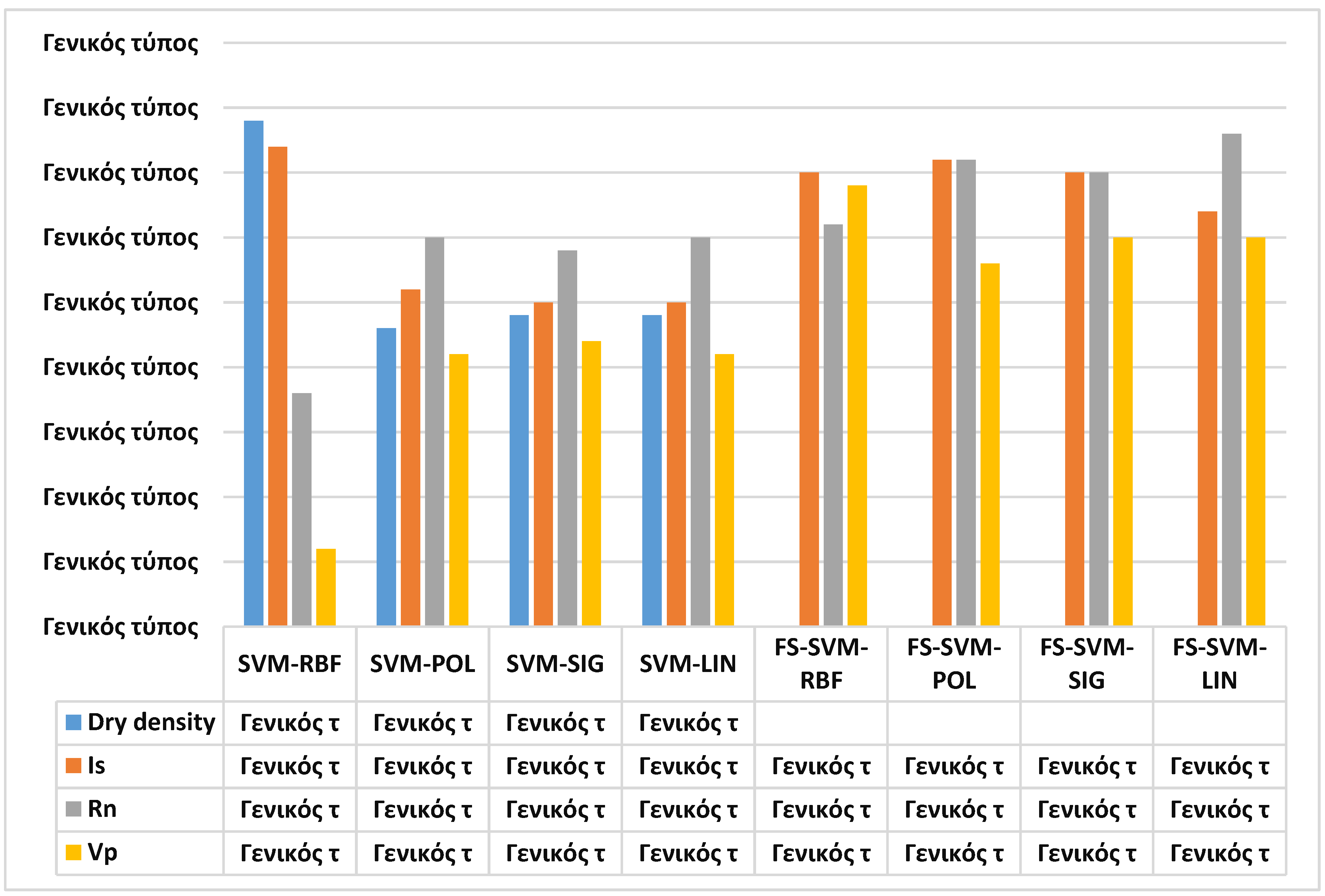
Each of the models developed identified the importance of the input variables to predict the rock BI. The importance of these variables is shown in Figure 9. As can be seen, while the three single-based models, including the SVM-POL, SVM-SIG, and SVM-LIN, identified Rn as the most important variable, the SVM-RBF identified density as the most important input variable. All four single-based SVM models identified the Vp as the least important variable. For the hybrid models, as the FS removed the density from the input lists, these models evaluated the importance of three inputs, including Rn, Vp, and, Is50 to predict the BI. Three hybrid-based models, including FS-SVM-RBF, FS-SVM-POL, and FS-SVM-SIG identified the Is50 as the most important input, while the FS-SVM-LIN identified the Rn as the most important input. Besides, FS-SVM-POL and FS-SVM-SIG identified Rn as the most important input along with the Is50. Vp was identified as the least important factor by FS-SVM-POL, FS-SVM-SIG, and FS-SVM-LIN, while the FS-SVM-RBF identified Rn as the least important input for predicting the BI.

5. Discussions

This study was set out to compare SVM models with different kernels to predict the rock BI. These kernels included RBF, POL, SIG, and LIN. The research team used two approaches for developing these SVM models. First, they developed single models, which meant that no input selection was conducted before developing these models. Second, they hybridized the SVM models with an FS technique.
The comparison of these approaches may help researchers to have a better insight into the advantages and disadvantages of the hybridization of different kernels of SVM techniques with an input selection technique (i.e., FS). The proposed models were compared in terms of accuracy performance, gains performance, and input variable importance. To develop the single-based models, four inputs, including D, Is50, Rn, and Vp were used to predict the BI, while the hybrid-based models were developed using three inputs (Is50, Rn, and Vp), because the FS technique removed one of the inputs (density) from the input list.
In terms of accuracy performance, the SVM models that were developed using the RBF kernel achieved the highest accumulative ranking regardless of whether they were single or hybrid. It is also worth noting that while the SVM-RBF model achieved the highest rank for both training and testing datasets, the FS-SVM-RBF model achieved the highest rank only for the training stage. Concerning the gains performance, the SVM models that used the RBF kernel again achieved the best results regardless whether they were single or hybrid. Thus, these findings imply that the RBF kernel is the most suitable choice to be used to develop the SVM models, regardless of whether these models are single or hybrid, for predicting the BI.
This study also evaluated the manner in which the SVM models identified the importance of each input variable. For single-based models, the SVM-RBF model differently identified the most important input from other single models. For the hybrid-based models, the FS-SVM-LIN differently identified the most important input. The accuracy and gains performance of SVM models that use the RBF kernel can support the power of these models to identify the importance of the input variables to predict the BI.

6. Conclusions

In this paper, an attempt has been made to predict the rock BI using empirical and ML techniques. The review of empirical relations revealed that although the performance capacity of the developed empirical equations is suitable, there is a need to develop an ML technique considering all model inputs, i.e., Vp, D, Rn, and Is50. Then, four single SVM models of SVM-RBF, SVM-POL, SVM-SIG, and SVM-LIN together with and four hybrid SVM models FS-SVM-RBF, FS-SVM-POL, FS-SVM-SIG, and FS-SVM-LIN were constructed to predict BI of the rock samples. The results of the cumulative rank values of 36, 30, 15, and 25 were obtained for the SVM-RBF, SVM-POL, SVM-SIG, and SVM-LIN models, respectively. In addition, cumulative rank values of 31, 29, 17 and 30 were achieved for the FS-SVM-RBF, FS-SVM-POL, FS-SVM-SIG, and FS-SVM-LIN models, respectively. This shows that the RBF is the most successful kernel for both single and hybrid SVM models to estimate the BI of the rock. As a concluding remark, the authors would like to stress that the modeling process presented in this study can be used in other areas of research as well, in order to succeed in solving a problem from a new point of view. Further studies that intend to use the SVM models should develop both single and hybrid models with different kernels. Then, they will understand the behavior of different kernels in a better way and will therefore select the most accurate and reliable model. In addition, future research should use a database with more samples that can help to improve the accuracy and generalizability of the prediction.

Author Contributions

Formal analysis, D.J.A. and B.A.; Conceptualization, M.H. and R.T.; Supervision, P.G.A.; Writing—review & editing, D.J.A., M.H. and P.G.A.; Resources, V.V.H. All authors have read and agreed to the published version of the manuscript.

Funding

This research received no external funding.

Acknowledgments

This research paper is made possible through the support of the Universiti Teknologi Malaysia (UTM) and the authors wish to appreciate their help and support.

Conflicts of Interest

The authors declare no conflict of interest.

References

  1. Miskimins, J.L. The impact of mechanical stratigraphy on hydraulic fracture growth and design considerations for horizontal wells. Bulletin 2012, 91, 475–499. [Google Scholar]
  2. Rickman, R.; Mullen, M.J.; Petre, J.E.; Grieser, W.V.; Kundert, D. A Practical Use of Shale Petrophysics for Stimulation Design Optimization: All Shale Plays Are Not Clones of the Barnett Shale. In Proceedings of the SPE Annual Technical Conference and Exhibition, Society of Petroleum Engineers (SPE), Denver, CO, USA, 21–24 September 2008. [Google Scholar]
  3. Rybacki, E.; Reinicke, A.; Meier, T.; Makasi, M.; Dresen, G. What controls the mechanical properties of shale rocks?—Part I: Strength and Young’s modulus. J. Petrol. Sci. Eng. 2015, 135, 702–722. [Google Scholar] [CrossRef]
  4. Rybacki, E.; Meier, T.; Dresen, G. What controls the mechanical properties of shale rocks?—Part II: Brittleness. J. Pet. Sci. Eng. 2016, 144, 39–58. [Google Scholar] [CrossRef] [Green Version]
  5. Hajiabdolmajid, V.; Kaiser, P. Brittleness of rock and stability assessment in hard rock tunneling. Tunn. Undergr. Space Technol. 2003, 18, 35–48. [Google Scholar] [CrossRef]
  6. Kidybinski, A. Bursting liability indices of coal. Int. J. Rock Mech. Min. Sci. Géoméch. Abstr. 1981, 18, 295–304. [Google Scholar] [CrossRef]
  7. Singh, S. Brittleness and the mechanical winning of coal. Min. Sci. Technol. 1986, 3, 173–180. [Google Scholar] [CrossRef]
  8. Zhou, J.; Li, X.; Mitri, H. Evaluation method of rockburst: State-of-the-art literature review. Tunn. Undergr. Space Technol. 2018, 81, 632–659. [Google Scholar] [CrossRef]
  9. Zhou, J.; Guo, H.; Koopialipoor, M.; Armaghani, D.J.; Tahir, M.M. Investigating the effective parameters on the risk levels of rockburst phenomena by developing a hybrid heuristic algorithm. Eng. Comput. 2020, 1–16. [Google Scholar] [CrossRef]
  10. Yagiz, S. Utilizing rock mass properties for predicting TBM performance in hard rock condition. Tunn. Undergr. Space Technol. 2008, 23, 326–339. [Google Scholar] [CrossRef]
  11. Ebrahimabadi, A.; Goshtasbi, K.; Shahriar, K.; Cheraghi Seifabad, M. A model to predict the performance of roadheaders based on the Rock Mass Brittleness Index. J. S. Afr. Inst. Min. Metall. 2011, 111, 355–364. [Google Scholar]
  12. Copur, C. A set of indices based on indentation tests for assessment of rock cutting performance and rock properties. J. S. Afr. Inst. Min. Metall. 2003, 103, 589–599. [Google Scholar]
  13. Yagiz, S. Assessment of brittleness using rock strength and density with punch penetration test. Tunn. Undergr. Space Technol. 2009, 24, 66–74. [Google Scholar] [CrossRef]
  14. Altindag, R. Assessment of some brittleness indexes in rock-drilling efficiency. Rock Mech. Rock Eng. 2009, 43, 361–370. [Google Scholar] [CrossRef]
  15. Morley, A. Strength of Material; Longmans: Suffolk, UK, 1944; pp. 1–518. [Google Scholar]
  16. Ramsay, J.G. Folding and Fracturing of Rocks; Mc Graw Hill Book Company: Desoto, TX, USA, 1967; 568p. [Google Scholar]
  17. Obert, L.; Duvall, W.I. Rock mechanics and the design of structures in rock. J. Wiley 1967, 278, 1–650. [Google Scholar]
  18. Yagiz, S.; Gokceoglu, C. Application of fuzzy inference system and nonlinear regression models for predicting rock brittleness. Expert Syst. Appl. 2010, 37, 2265–2272. [Google Scholar] [CrossRef]
  19. Wang, Y.; Watson, R.; Rostami, J.; Wang, J.Y.; Limbruner, M.; He, Z. Study of borehole stability of Marcellus shale wells in longwall mining areas. J. Pet. Explor. Prod. Technol. 2013, 4, 59–71. [Google Scholar] [CrossRef] [Green Version]
  20. Meng, F.; Zhou, H.; Zhang, C.; Xu, R.; Lu, J. Evaluation Methodology of Brittleness of Rock Based on Post-Peak Stress–Strain Curves. Rock Mech. Rock Eng. 2014, 48, 1787–1805. [Google Scholar] [CrossRef]
  21. Koopialipoor, M.; Noorbakhsh, A.; Ghaleini, E.N.; Armaghani, D.J.; Yagiz, S. A new approach for estimation of rock brittleness based on non-destructive tests. Nondestruct. Test. Eval. 2019, 34, 354–375. [Google Scholar] [CrossRef]
  22. Khandelwal, M.; Faradonbeh, R.S.; Monjezi, M.; Armaghani, D.J.; Majid, M.Z.B.A.; Yagiz, S. Function development for appraising brittleness of intact rocks using genetic programming and non-linear multiple regression models. Eng. Comput. 2016, 33, 13–21. [Google Scholar] [CrossRef]
  23. Lawn, B.R.; Marshall, D.B. Hardness, Toughness, and Brittleness: An Indentation Analysis. J. Am. Ceram. Soc. 1979, 62, 347–350. [Google Scholar] [CrossRef]
  24. Nejati, H.R.; Moosavi, S.A. A new brittleness index for estimation of rock fracture toughness. J. Min. Reclam. Environ. 2017, 8, 83–91. [Google Scholar]
  25. Hucka, V.; Das, B. Brittleness determination of rocks by different methods. Int. J. Rock Mech. Min. Sci. Géoméch. Abstr. 1974, 11, 389–392. [Google Scholar] [CrossRef]
  26. Zhou, J.; Li, X.; Mitri, H. Comparative performance of six supervised learning methods for the development of models of hard rock pillar stability prediction. Nat. Hazards 2015, 79, 291–316. [Google Scholar] [CrossRef]
  27. Zhou, J.; Shi, X.; Li, X. Utilizing gradient boosted machine for the prediction of damage to residential structures owing to blasting vibrations of open pit mining. J. Vib. Control. 2016, 22, 3986–3997. [Google Scholar] [CrossRef]
  28. Zhou, J.; Shi, X.; Du, K.; Qiu, X.; Li, X.; Mitri, H. Feasibility of Random-Forest Approach for Prediction of Ground Settlements Induced by the Construction of a Shield-Driven Tunnel. Int. J. Géoméch. 2017, 17, 04016129. [Google Scholar] [CrossRef]
  29. Zhou, J.; Li, E.; Yang, S.; Wang, M.; Shi, X.; Yao, S.; Mitri, H. Slope stability prediction for circular mode failure using gradient boosting machine approach based on an updated database of case histories. Saf. Sci. 2019, 118, 505–518. [Google Scholar] [CrossRef]
  30. Shi, X.-Z.; Zhou, J.; Wu, B.; Huang, D.; Wei, W. Support vector machines approach to mean particle size of rock fragmentation due to bench blasting prediction. Trans. Nonferrous Met. Soc. China 2012, 22, 432–441. [Google Scholar] [CrossRef]
  31. Xu, H.; Zhou, J.; Asteris, P.; Armaghani, D.J.; Tahir, M.M. Supervised Machine Learning Techniques to the Prediction of Tunnel Boring Machine Penetration Rate. Appl. Sci. 2019, 9, 3715. [Google Scholar] [CrossRef] [Green Version]
  32. Hajihassani, M.; Abdullah, S.; Asteris, P.; Armaghani, D.J. A Gene Expression Programming Model for Predicting Tunnel Convergence. Appl. Sci. 2019, 9, 4650. [Google Scholar] [CrossRef] [Green Version]
  33. Armaghani, D.J.; Hatzigeorgiou, G.D.; Karamani, C.; Skentou, A.; Zoumpoulaki, I.; Asteris, P. Soft computing-based techniques for concrete beams shear strength. Procedia Struct. Integr. 2019, 17, 924–933. [Google Scholar] [CrossRef]
  34. Asteris, P.G.; Armaghani, D.J.; Hatzigeorgiou, G.D.; Karayannis, C.G.; Pilakoutas, K. Predicting the shear strength of reinforced concrete beams using Artificial Neural Networks. Eng. Struct. 2019, 24, 469–488. [Google Scholar]
  35. Chen, H.; Asteris, P.; Armaghani, D.J.; Gordan, B.; Pham, B.T. Assessing Dynamic Conditions of the Retaining Wall: Developing Two Hybrid Intelligent Models. Appl. Sci. 2019, 9, 1042. [Google Scholar] [CrossRef] [Green Version]
  36. Huang, L.; Asteris, P.; Koopialipoor, M.; Armaghani, D.J.; Tahir, M.M. Invasive Weed Optimization Technique-Based ANN to the Prediction of Rock Tensile Strength. Appl. Sci. 2019, 9, 5372. [Google Scholar] [CrossRef] [Green Version]
  37. Apostolopoulou, M.; Armaghani, D.J.; Bakolas, A.; Douvika, M.G.; Moropoulou, A.; Asteris, P. Compressive strength of natural hydraulic lime mortars using soft computing techniques. Procedia Struct. Integr. 2019, 17, 914–923. [Google Scholar] [CrossRef]
  38. Sarir, P.; Chen, J.; Asteris, P.G.; Armaghani, D.J.; Tahir, M.M. Developing GEP tree-based, neuro-swarm, and whale optimization models for evaluation of bearing capacity of concrete-filled steel tube columns. Eng. Comput. 2019, 1–19. [Google Scholar] [CrossRef]
  39. Asteris, P.G.; Ashrafian, A.; Rezaie-Balf, M. Prediction of the compressive strength of self-compacting concrete using surrogate models. Comput. Concr. 2019, 24, 137–150. [Google Scholar]
  40. Asteris, P.; Moropoulou, A.; Skentou, A.D.; Apostolopoulou, M.; Mohebkhah, A.; Cavaleri, L.; Rodrigues, H.; Varum, H. Stochastic vulnerability assessment of masonry structures: Concepts, modeling and restoration aspects. Appl. Sci. 2019, 9, 243. [Google Scholar] [CrossRef] [Green Version]
  41. Asteris, P.; Mokos, V.G. Concrete compressive strength using artificial neural networks. Neural Comput. Appl. 2019, 1–20. [Google Scholar] [CrossRef]
  42. Asteris, P.; Kolovos, K. Self-compacting concrete strength prediction using surrogate models. Neural Comput. Appl. 2017, 31, 409–424. [Google Scholar] [CrossRef]
  43. Asteris, P.; Nozhati, S.; Nikoo, M.; Cavaleri, L.; Nikoo, M. Krill herd algorithm-based neural network in structural seismic reliability evaluation. Mech. Adv. Mater. Struct. 2018, 26, 1146–1153. [Google Scholar] [CrossRef]
  44. Apostolopoulour, M.; Douvika, M.G.; Kanellopoulos, I.N.; Moropoulou, A.; Asteris, P.G. Prediction of Compressive Strength of Mortars using Artificial Neural Networks. In Proceedings of the 1st International Conference TMM_CH, Transdisciplinary Multispectral Modelling and Cooperation for the Preservation of Cultural Heritage, Athens, Greece, 10–13 October 2018. [Google Scholar]
  45. Mohamad, E.T.; Armaghani, D.J.; Momeni, E.; Yazdavar, A.H.; Ebrahimi, M. Rock strength estimation: A PSO-based BP approach. Neural Comput. Appl. 2016, 30, 1635–1646. [Google Scholar] [CrossRef]
  46. Armaghani, D.J.; Mohamad, E.T.; Momeni, E.; Monjezi, M.; Narayanasamy, M.S. Prediction of the strength and elasticity modulus of granite through an expert artificial neural network. Arab. J. Geosci. 2015, 9, 48. [Google Scholar] [CrossRef]
  47. Momeni, E.; Nazir, R.; Armaghani, D.J.; Maizir, H. Application of artificial neural network for predicting shaft and tip resistances of concrete piles. Earth Sci. Res. J. 2015, 19, 85–93. [Google Scholar] [CrossRef]
  48. Momeni, E.; Armaghani, D.J.; Fatemi, S.A.; Nazir, R. Prediction of bearing capacity of thin-walled foundation: A simulation approach. Eng. Comput. 2017, 34, 319–327. [Google Scholar] [CrossRef]
  49. Mohamad, E.T.; Li, D.; Murlidhar, B.R.; Armaghani, D.J.; Kassim, K.A.; Komoo, I. The effects of ABC, ICA, and PSO optimization techniques on prediction of ripping production. Eng. Comput. 2019, 1–16. [Google Scholar] [CrossRef]
  50. Koopialipoor, M.; Tootoonchi, H.; Armaghani, D.J.; Mohamad, E.T.; Hedayat, A. Application of deep neural networks in predicting the penetration rate of tunnel boring machines. Bull. Int. Assoc. Eng. Geol. 2019, 78, 6347–6360. [Google Scholar] [CrossRef]
  51. Guo, H.; Zhou, J.; Koopialipoor, M.; Armaghani, D.J.; Tahir, M.M. Deep neural network and whale optimization algorithm to assess flyrock induced by blasting. Eng. Comput. 2019, 1–14. [Google Scholar] [CrossRef]
  52. Harandizadeh, H.; Armaghani, D.J.; Khari, M. A new development of ANFIS–GMDH optimized by PSO to predict pile bearing capacity based on experimental datasets. Eng. Comput. 2019, 1–16. [Google Scholar] [CrossRef]
  53. Chen, W.; Sarir, P.; Bui, X.-N.; Nguyen, H.; Tahir, M.M.; Armaghani, D.J. Neuro-genetic, neuro-imperialism and genetic programing models in predicting ultimate bearing capacity of pile. Eng. Comput. 2019, 1–15. [Google Scholar] [CrossRef]
  54. Sun, L.; Koopialipoor, M.; Armaghani, D.J.; Tarinejad, R.; Tahir, M.M. Applying a meta-heuristic algorithm to predict and optimize compressive strength of concrete samples. Eng. Comput. 2019, 1–13. [Google Scholar]
  55. Asteris, P.; Nikoo, M. Artificial bee colony-based neural network for the prediction of the fundamental period of infilled frame structures. Neural Comput. Appl. 2019, 31, 4837–4847. [Google Scholar] [CrossRef]
  56. Gowida, A.; Elkatatny, S.; Al-Afnan, S.; Abdulraheem, A. New computational artificial intelligence models for generating synthetic formation bulk density logs while drilling. Sustainability 2020, 12, 686. [Google Scholar] [CrossRef] [Green Version]
  57. Garg, R.; Aggarwal, H.; Centobelli, P.; Cerchione, R. Extracting knowledge from big data for sustainability: A comparison of machine learning techniques. Sustainability 2019, 11, 6669. [Google Scholar] [CrossRef] [Green Version]
  58. Yang, H.; Zeng, Y.; Lan, Y.; Zhou, X. Analysis of the excavation damaged zone around a tunnel accounting for geostress and unloading. Int. J. Rock Mech. Min. Sci. 2014, 69, 59–66. [Google Scholar] [CrossRef]
  59. Yang, H.; Xing, S.; Wang, Q.; Li, Z. Model test on the entrainment phenomenon and energy conversion mechanism of flow-like landslides. Eng. Geol. 2018, 239, 119–125. [Google Scholar] [CrossRef]
  60. Yang, H.; Li, Z.; Jie, T.; Zhang, Z. Effects of joints on the cutting behavior of disc cutter running on the jointed rock mass. Tunn. Undergr. Space Technol. 2018, 81, 112–120. [Google Scholar] [CrossRef]
  61. Liu, B.; Yang, H.; Karekal, S. Effect of Water Content on Argillization of Mudstone During the Tunnelling process. Rock Mech. Rock Eng. 2019, 53, 799–813. [Google Scholar] [CrossRef]
  62. Armaghani, D.J.; Mohamad, E.T.; Narayanasamy, M.S.; Narita, N.; Yagiz, S. Development of hybrid intelligent models for predicting TBM penetration rate in hard rock condition. Tunn. Undergr. Space Technol. 2017, 63, 29–43. [Google Scholar] [CrossRef]
  63. Asteris, P.; Argyropoulos, I.; Cavaleri, L.; Rodrigues, H.; Varum, H.; Thomas, J.; Lourenço, P.B. Masonry Compressive Strength Prediction Using Artificial Neural Networks. In Proceedings of the 1st International Conference TMM_CH, Transdisciplinary Multispectral Modelling and Cooperation for the Preservation of Cultural Heritage, Athens, Greece, 10–13 October 2018; Springer Science and Business Media LLC: New York, NY, USA, 2019; pp. 200–224. [Google Scholar]
  64. Asteris, P.; Roussis, P.C.; Douvika, M.G. Feed-Forward Neural Network Prediction of the Mechanical Properties of Sandcrete Materials. Sensors 2017, 17, 1344. [Google Scholar] [CrossRef] [Green Version]
  65. Cavaleri, L.; Chatzarakis, G.E.; Di Trapani, F.; Douvika, M.G.; Roinos, K.; Vaxevanidis, N.M.; Asteris, P.G. Modeling of surface roughness in electro-discharge machining using artificial neural networks. Adv. Mater. Res. 2017, 6, 169–184. [Google Scholar]
  66. Cavaleri, L.; Asteris, P.; Psyllaki, P.P.; Douvika, M.G.; Skentou, A.D.; Vaxevanidis, N.M. Prediction of surface treatment effects on the tribological performance of tool steels using artificial neural networks. Appl. Sci. 2019, 9, 2788. [Google Scholar] [CrossRef] [Green Version]
  67. Psyllaki, P.P.; Stamatiou, K.; Iliadis, I.; Mourlas, A.; Asteris, P.; Vaxevanidis, N. Surface Treatment of Tool Steels Against Galling Failure. In Proceedings of the 5th International Conference of Engineering Against Failure (ICEAF V), Chios Island, Greece, 20–22 June 2018; EDP Sciences: Les Ulis, France, 2018; Volume 188, p. 04024. [Google Scholar]
  68. Asteris, P.; Tsaris, A.K.; Cavaleri, L.; Repapis, C.C.; Papalou, A.; Di Trapani, F.; Karypidis, D.F. Prediction of the Fundamental Period of Infilled RC Frame Structures Using Artificial Neural Networks. Comput. Intell. Neurosci. 2015, 2016, 1–12. [Google Scholar] [CrossRef] [PubMed] [Green Version]
  69. Nguyen, M.D.; Pham, B.T.; Tuyen, T.T.; Yen, H.P.H.; Prakash, I.; Vu, T.T.; Chapi, K.; Shirzadi, A.; Shahabi, H.; Dou, J.; et al. Development of an Artificial Intelligence Approach for Prediction of Consolidation Coefficient of Soft Soil: A Sensitivity Analysis. Open Constr. Build. Technol. J. 2019, 13, 178–188. [Google Scholar] [CrossRef]
  70. Kechagias, J.; Tsiolikas, A.; Asteris, P.; Vaxevanidis, N. Optimizing ANN performance using DOE: Application on turning of a titanium alloy. In Proceedings of the IMANEE-2018, Chisinau, Moldova, 31 May–2 June 2018; EDP Sciences: Les Ulis, France, 2018; Volume 178, p. 01017. [Google Scholar]
  71. Asteris, P.; Kolovos, K.; Douvika, M.; Roinos, K. Prediction of self-compacting concrete strength using artificial neural networks. Eur. J. Environ. Civ. Eng. 2016, 20, s102–s122. [Google Scholar] [CrossRef]
  72. Zhou, J.; Li, C.; Koopialipoor, M.; Armaghani, D.J.; Pham, B.T. Development of a new methodology for estimating the amount of PPV in surface mines based on prediction and probabilistic models (GEP-MC). Int. J. Min. Reclam. Environ. 2020, 1–21. [Google Scholar] [CrossRef]
  73. Armaghani, D.J.; Mirzaei, F.; Shariati, M.; Trung, N.T.; Shariati, M.; Trnavac, D. Hybrid ANN-based techniques in predicting cohesion of sandy-soil combined with fiber. Geomech. Eng. 2020, 20, 191–205. [Google Scholar]
  74. Armaghani, D.J.; Kumar, D.; Samui, P.; Hasanipanah, M.; Roy, B. A novel approach for forecasting of ground vibrations resulting from blasting: Modified particle swarm optimization coupled extreme learning machine. Eng. Comput. 2020, 1–15. [Google Scholar] [CrossRef]
  75. Dao, D.V.; Adeli, H.; Ly, H.-B.; Le, L.M.; Le, V.M.; Le, T.-T.; Pham, B.T. A sensitivity and robustness analysis of GPR and ANN for high-performance concrete compressive strength prediction using a monte carlo simulation. Sustainability 2020, 12, 830. [Google Scholar] [CrossRef] [Green Version]
  76. Altindag, R. The role of rock brittleness on analysis of percussive drilling performance. In Proceedings of the 5th Turkish National Rock Mechanics Symposium, Isparta, Turkey, 30–31 October 2000; pp. 105–112. [Google Scholar]
  77. Yarali, O.; Soyer, E. The effect of mechanical rock properties and brittleness on drillability. Sci. Res. Essays 2011, 6, 1077–1088. [Google Scholar]
  78. Jebur, M.N.; Pradhan, B.; Tehrany, M.S. Optimization of landslide conditioning factors using very high-resolution airborne laser scanning (LiDAR) data at catchment scale. Remote. Sens. Environ. 2014, 152, 150–165. [Google Scholar] [CrossRef]
  79. Marjanovic, M.; Kovačević, M.; Bajat, B.; Voženílek, V. Landslide susceptibility assessment using SVM machine learning algorithm. Eng. Geol. 2011, 123, 225–234. [Google Scholar] [CrossRef]
  80. Armaghani, D.J.; Koopialipoor, M.; Marto, A.; Yagiz, S. Application of several optimization techniques for estimating TBM advance rate in granitic rocks. J. Rock Mech. Geotech. Eng. 2019, 11, 779–789. [Google Scholar] [CrossRef]
  81. Kaunda, R.B.; Asbury, B. Prediction of rock brittleness using nondestructive methods for hard rock tunneling. J. Rock Mech. Geotech. Eng. 2016, 8, 533–540. [Google Scholar] [CrossRef] [Green Version]
  82. Bui, D.T.T.; Pradhan, B.; Löfman, O.; Revhaug, I. Landslide Susceptibility Assessment in Vietnam Using Support Vector Machines, Decision Tree, and Naïve Bayes Models. Math. Probl. Eng. 2012, 2012, 1–26. [Google Scholar]
  83. Hasanipanah, M.; Monjezi, M.; Shahnazar, A.; Armaghani, D.J.; Farazmand, A. Feasibility of indirect determination of blast induced ground vibration based on support vector machine. Measurement 2015, 75, 289–297. [Google Scholar] [CrossRef]
  84. Song, S.; Zhan, Z.; Long, Z.; Zhang, J.; Yao, L. Comparative Study of SVM Methods Combined with Voxel Selection for Object Category Classification on fMRI Data. PLoS ONE 2011, 6, 6. [Google Scholar] [CrossRef]
  85. Tehrany, M.S.; Pradhan, B.; Jebur, M.N. Flood susceptibility mapping using a novel ensemble weights-of-evidence and support vector machine models in GIS. J. Hydrol. 2014, 512, 332–343. [Google Scholar] [CrossRef]
  86. Ulusay, R.; Hudson, J.A. The Complete ISRM Suggested Methods for Rock Characterization, Testing and Monitoring: 1974–2006; International Society for Rock Mechanics, Commission on Testing Methods: Ankara, Turkey, 2007; p. 628. [Google Scholar]
  87. Zorlu, K.; Gokceoglu, C.; Ocakoglu, F.; Nefeslioglu, H.; Acikalin, S. Prediction of uniaxial compressive strength of sandstones using petrography-based models. Eng. Geol. 2008, 96, 141–158. [Google Scholar] [CrossRef]
Figure 1. Schematic of the support vector machine (SVM).
Sustainability 12 02229 g001
Figure 2. SVM structure for regression.
Sustainability 12 02229 g002
Figure 3. Failure of a sample under a Brazilian tensile strength (BTS) test.
Sustainability 12 02229 g003
Figure 4. Conducted uniaxial compressive strength (UCS) test on a rock sample (a) before failure and (b) after failure.
Sustainability 12 02229 g004
Figure 5. R values and scatter plots of the input and output parameters.
Sustainability 12 02229 g005
Figure 6. Performance indices.
Sustainability 12 02229 g006
Figure 7. Evaluation of single-based SVM models with different kernels using gains.
Sustainability 12 02229 g007
Figure 8. Evaluation of hybrid-based SVM models with different kernels using gains.
Sustainability 12 02229 g008
Figure 9. Importance of input variables based on the eight SVM models developed.
Sustainability 12 02229 g009
Table 1. Kernels’ formula.
KernelEquation
RBF G ( x i , x j ) = e x p ( γ x i x j 2 )
POL G ( x i , x j ) = ( γ x i t x j + 1 ) d
SIG G ( x i , x j ) = T a n h ( γ x i t x + 1 ) d
LIN G ( x i , x j ) = x i t x j
Table 2. The proposed correlations between the input variables and the brittleness index (BI).
VariableEquationR
RnBI = 2.6947 Rn − 1.1290.815
VpBI = 291.98 Vp + 976.890.747
DBI = 0.0231 D + 2.2330.730
Is50BI = 0.3604 Is50 − 1.9240.749
Table 3. Parameters used for developing the single-based SVM models.
ParameterSVM-RBFSVM-POLSVM-SIGSVM-LIN
Stopping criteria1.0 × 10−31.0 × 10−31.0 × 10−31.0 × 10⁻³
Regularization parameter (C)10.010.010.01.0
Regression precision (epsilon)0.10.10.10.05
RBF gamma1.5---
Gamma-0.20.05-
Bias-0.00.01-
Degree-1.0--
Table 4. Parameters used for developing the hybrid-based SVM models.
ParameterSVM-RBFSVM-POLSVM-SIGSVM-LIN
Stopping criteria1.0 × 10−31.0 × 10−31.0 × 10−31.0 × 10⁻³
Regularization parameter (C)10.010.010.010.0
Regression precision (epsilon)0.10.10.11.0
RBF gamma1.25---
Gamma-0.20.05-
Bias-0.00.01-
Degree-1.0--
Table 5. Evaluation of single models developed using five performance indices.
SVM-RBFSVM-POLSVM-SIGSVM-LIN
TRTETRTETRTETRTE
ValueRankValueRankValueRankValueRankValueRankValueRankValueRankValueRank
R0.8840.9240.8630.9230.8520.9110.8630.922
RMSE1.4141.3541.5831.3831.7211.5411.6321.412
VAF77.6486.1372.0387.2466.5181.2170.2285.32
MAE1.1141.0341.3331.0431.4511.3011.3721.132
a20-index0.9430.9420.9220.9730.9430.9730.9540.974
Sum of the ranksTRTETRTETRTETRTE
19171416871312
Cumulative rank36301525
Support vector machine = SVM; Radial basis function = RBF; Polynomial = POL; Sigmoid = SIG; Linear = LIN; Perfect R = 1; Perfect RMSE = 0; Perfect VAF = 100%; Perfect MAE = 0; a20-index = 1. Training dataset = TR; Testing dataset = TE.
Table 6. Evaluation of hybrid models developed using five performance indices.
FS-SVM-RBFFS-SVM-POLFS-SVM-SIGFS-SVM-LIN
TRTETRTETRTETRTE
ValueRankValueRankValueRankValueRankValueRankValueRankValueRankValueRank
R0.8640.9110.8530.9240.8520.9230.8520.912
RMSE1.5641.4121.6421.3841.7711.5511.5931.403
VAF73.0485.2269.7285.6364.7180.4171.4386.74
MAE1.2141.1421.3521.1131.4611.3011.3531.074
a20-index0.9440.9740.9220.9740.9220.9740.9330.963
Sum of the ranksTRTETRTETRTETRTE
201111187101416
Cumulative rank31291730
Support vector machine = SVM; Radial basis function = RBF; Polynomial = POL; Sigmoid = SIG; Linear = LIN; Feature selection = FS. Perfect R = 1; Perfect RMSE = 0; Perfect VAF = 100%; Perfect MAE = 0; a20-index = 1. Training dataset = TR; Testing dataset = TE.

