A Comparison of Wind Energy Investment Alternatives Using Interval-Valued Intuitionistic Fuzzy Benefit/Cost Analysis

Abstract

One of the tools for maintaining environmental sustainability is transformation from fossil-based energy sources to renewable energy sources in energy consumption. Among renewable energy alternatives, wind energy is the most prominent and reliable energy source for fulfilling energy demand. Traditional investment evaluation techniques based on discounted cash flows are not capable of capturing the uncertainty and vagueness in the data related to the wind energy investment parameters. Fuzzy capital budgeting techniques can capture this vagueness and model the imprecise estimations of parameter values. In this paper, we develop interval-valued intuitionistic fuzzy benefit-cost analysis for the evaluation of wind energy technology investments. The fuzzy benefit-cost analyses are based on both present worth and annual worth analyses. The developed analyses can handle the assessments of multiple experts through aggregation operators. In the proposed economic model, the components of each wind energy investment parameter are incorporated into the equations in detail. A real case study is also presented in this paper.

1. Introduction

Managing environmental resources, especially energy sources, is one of the main determinants of a sustainable development. In order to support sustainability, many researchers focused on energy issues [1]. Renewable energy resources provide clean, affordable, and inexhaustible energy source and decrease emission of greenhouse gases and protect global warming. Among the renewable energy resources, wind energy is a reliable source of energy that enables sustainable development and it accounts for 36% of total generated renewable energy [2]. In 2014, the global cumulative installed wind capacity has reached 369,597 MW. Table 1 shows the global cumulative installed wind capacity (MW) [3].

Table 1. Global cumulative installed wind capacity.

Year	1997	1998	1999	2000	2001	2002	2003	2004	2005
Cum.Capacity (MW)	7600	10,200	13,600	17,400	23,900	31,100	39,431	47,620	59,091
Year	2006	2007	2008	2009	2010	2011	2012	2013	2014
Cum.Capacity (MW)	73,949	93,901	120,715	159,079	197,943	238,435	283,132	318,644	369,597

Table 1. Global cumulative installed wind capacity.

Year	1997	1998	1999	2000	2001	2002	2003	2004	2005
Cum.Capacity (MW)	7600	10,200	13,600	17,400	23,900	31,100	39,431	47,620	59,091
Year	2006	2007	2008	2009	2010	2011	2012	2013	2014
Cum.Capacity (MW)	73,949	93,901	120,715	159,079	197,943	238,435	283,132	318,644	369,597

The Turkish wind energy market is a fast growing market with a 3763 MW total installed capacity. In 2014, Turkey added 804 MW of new wind power [3]. Turkey, especially the western part of Turkey, has a great wind energy potential [4,5,6]. Although the installed wind energy capacity has been increasing over the years, falls in fossil fuel prices have raised questions over the competitiveness of wind energy investments. A detailed economic analysis of wind energy investments may reflect the economic feasibility of wind energy investments.

Economic analysis of wind energy investments includes many parameters such as turbine costs, foundation costs, connection to the system costs, planning and license costs, and operating and maintenance costs including rent costs. The forecasted annual operating and maintenance costs and annual incomes that depend on the feed-in tariff should be correctly discounted based on a time value of money. The economic analysis technique can be any of present worth analysis, annual cash flow analysis, rate of return analysis, or benefit-cost (B/C) ratio analysis. The classical benefit-cost ratio can be defined as the ratio of the equivalent value of benefits to the equivalent value of costs. In this paper, B/C analysis is used since this technique is generally used for public projects and exhibits a clear comparison between benefits and costs.

The benefit-cost (B/C) ratio can be formulated as PWB/PWC or EUAB/EUAC where PWB and EUAB represent the present worth of benefits and equivalent uniform annual benefit associated with the project, respectively, and PWC and EUAC represent the present worth of costs and equivalent uniform annual costs, respectively [7]. A B/C ratio greater than or equal to 1.0 indicates that the project evaluated is economically advantageous. When there are two or more mutually exclusive alternatives, the incremental B/C analysis between the alternatives is realized.

The wind energy investment parameters are generally forecasted under uncertainty. If sufficient data are available, risk models are preferred by the experts. But, in case of insufficient, incomplete, imprecise or vague data, the experts cannot use risk models. They need the models that can take these types of data into account, which the fuzzy set theory excellently offers. In the fuzzy set theory founded by Zadeh [8], an element can be a member of various sets at the same time, and everything is a matter of degree. Fuzzy sets have been widely used in many problems such as strategic decision-making [9], risk management [10], investment evaluations [11], multicriteria decision-making [12], supply chain [13], flexible manufacturing [14] and modeling capabilities [15]. The ordinary fuzzy sets have been recently extended to intuitionistic fuzzy sets [2,16], hesitant fuzzy sets [17,18], fuzzy multisets [19], type-2 fuzzy sets [20,21], and stationary fuzzy sets [22]. Kahraman et al. [23] developed fuzzy B/C ratio analysis using ordinary fuzzy sets for the cases of single alternative and multiple alternatives having equal and unequal useful lives.

In this paper, we prefer using interval-valued intuitionistic fuzzy sets for the economic analysis of wind energy technologies since they let us define the membership and non-membership degrees together with the hesitancy. When decision makers are forced to make sharp and precise evaluations in case of insufficient information, they may not be able to accurately express their preferences. This is less but still true when ordinary fuzzy sets are used as a tool to express their preferences. Intuitionistic fuzzy sets provide an efficient tool to capture this problem by incorporating membership, non-membership, and hesitancy into decision makers’ evaluations. Intuitionistic fuzzy sets are the generalization of ordinary fuzzy sets. Intuitionistic fuzzy sets can deal with inevitably imprecise or not totally reliable information. Therefore, it better simulates human decision-making processes and any activities requiring human expertise and knowledge in these cases. These membership degrees can be expressed in different ways: single values, intervals, triangular or trapezoidal fuzzy numbers, etc. We developed fuzzy B/C ratio analysis using interval-valued intuitionistic fuzzy sets (IVIFS) for the cases of single alternative and multiple alternatives having equal and unequal useful lives.

The rest of this paper is organized as follows. Section 2 gives the literature review results on wind energy investments. Section 3 presents IVIFS and their aggregation and defuzzification operators. Section 4 develops intuitionistic fuzzy benefit-cost ratio analysis based on both present worth and annual worth. Section 5 includes an application of IVIF B/C ratio analysis for wind energy investments. Section 6 concludes the paper and presents suggestions for further research.

2. Wind Energy Investments

Total wind energy installed capacity is increasing dramatically with an average more than 10% annual increase. Table 2 illustrates global annual installed wind capacity [3]. In 2014, globally, 51,473 MW of wind capacity has been installed. Although the wind energy installation capacity is increasing, the wind energy usage has not reached its potential due to the relatively high investment costs and low fossil fuel prices. A comprehensive economic analysis may enable appropriate technology selection and can increase the wind energy usage.

Table 2. Global annual installed wind capacity.

Year	1997	1998	1999	2000	2001	2002	2003	2004	2005
Capacity (MW)	1530	2520	3440	3760	6500	7270	8133	8207	11,531
Year	2006	2007	2008	2009	2010	2011	2012	2013	2014
Capacity (MW)	14,701	20,286	26,952	38,478	38,989	40,943	44,929	35,692	51,473

Table 2. Global annual installed wind capacity.

Year	1997	1998	1999	2000	2001	2002	2003	2004	2005
Capacity (MW)	1530	2520	3440	3760	6500	7270	8133	8207	11,531
Year	2006	2007	2008	2009	2010	2011	2012	2013	2014
Capacity (MW)	14,701	20,286	26,952	38,478	38,989	40,943	44,929	35,692	51,473

The wind power potential of a wind turbine is related with its characteristic and its compatibility to the environmental conditions [24,25]. The environmental conditions involve wind velocity and air density. The swept area, cut-in speed, cut-out speed, rotor diameter and height of the turbine are the technological characteristics [26,27]. The wind tribunes are active for certain cut-in and cut-off speeds, and they cannot fully utilize all the energy of blowing wind due to rotor blade friction, gearbox losses, the generator and the converter. Different wind turbine technologies provide different wind energy production. When selecting the wind turbines, the available wind turbines, their technological characteristics and the potential wind energy production levels should first be defined. In order to select the best wind turbine, this technical analysis should be combined with an economic analysis.

In the literature, there are several studies that economically analyze wind turbine investments. Mostafaeipour et al. [28] analyzed the wind energy potential for the city of Zahedan and selected the most economic wind turbine technology among four small size wind turbines. The initial investment costs, maintenance and operation costs were used for the selection process. Rahimi et al. [29] applied a techno-economic evaluation to an in household size wind-hydrogen hybrid system. They considered annualized capital, annualized replacement and annualized maintenance costs. Schallenberg-Rodriguez [30] proposed a methodology to calculate the annualized wind generation cost and applied this methodology to the wind energy investments in the Canary Islands. Mohammadi and Mostafaeipour [31] evaluated six different wind turbines in order to reveal the economic feasibility of electricity generation using wind turbines in city of Aligoodarz. Ertürk [5] analyzed the onshore wind energy potential of Turkey and the impact of regulations and incentives on this potential. In this study, the net present values under different scenarios were evaluated.

The wind energy investment costs can be defined as the turbine costs, grid connection, foundation, land rent, electric installation, consultancy, financial costs, road construction, control systems, operational and maintenance expenses [4,5,32,33]. These costs change based on the turbine capacity, land characteristics and the turbine characteristics. In this study, investment costs, turbine costs, foundation costs, connection to the system, rental costs, planning and license costs were considered the main fixed costs, whereas operating and maintenance costs were considered the main variable costs.

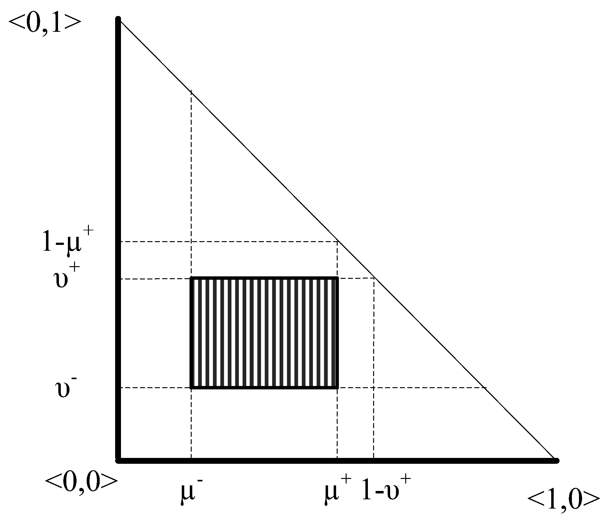
3. Interval Valued Intuitionistic Fuzzy Sets

In the fuzzy set theory, the membership of an element to a fuzzy set is a single value between zero and one. However, the degree of non-membership of an element in a fuzzy set may not be equal to 1 minus the membership degree since there may be some hesitation degree. Therefore, a generalization of fuzzy sets was proposed by Atanassov [34] as intuitionistic fuzzy sets (IFS) that incorporate the degree of hesitation, which is defined as 1 minus the sum of membership and non-membership degrees.

Let $\mathrm{D}\subseteq \left[0,1\right]$ be the set of all closed subintervals of the interval and X be a universe of discourse. An interval-valued intuitionistic fuzzy set $\tilde{\mathrm{A}}$ over X is an object having the form

$$\tilde{\mathrm{A}}=\left\{<x, {\mathsf{\mu }}_{\tilde{\mathrm{A}}}\left(\mathrm{x}\right),{\mathrm{v}}_{\tilde{\mathrm{A}}}\left(\mathrm{x}\right)>|\mathrm{x}\in \mathrm{X}\right\}$$

(1)

where ${\mathsf{\mu }}_{\tilde{\mathrm{A}}}\to \mathrm{D}\subseteq \left[0,1\right],$ ${\mathrm{v}}_{\tilde{\mathrm{A}}}\left(\mathrm{x}\right)\to \mathrm{D}\subseteq \left[0,1\right]$ with the condition $0\le {\text{sup}\mathsf{\mu }}_{\tilde{\mathrm{A}}}\left(\mathrm{x}\right)+{\text{supv}}_{\tilde{\mathrm{A}}}\left(\mathrm{x}\right)\le 1,\forall \mathrm{x}\in \mathrm{X}.$

The intervals ${\mathsf{\mu }}_{\tilde{\mathrm{A}}}\left(\mathrm{x}\right)$ and ${\mathrm{v}}_{\tilde{\mathrm{A}}}\left(\mathrm{x}\right)$ denote the membership function and the non-membership function of the element x to the set $\tilde{\mathrm{A}}$, respectively. Thus, for each $\mathrm{x}\in \mathrm{X}$, ${\mathsf{\mu }}_{\tilde{\mathrm{A}}}\left(\mathrm{x}\right)$ and ${\mathrm{v}}_{\tilde{\mathrm{A}}}\left(\mathrm{x}\right)$ are closed intervals, and their starting and ending points are denoted by ${\mathsf{\mu }}_{\tilde{\mathrm{A}}}^{-}\left(\mathrm{x}\right),{ \mathsf{\mu }}_{\tilde{\mathrm{A}}}^{+}\left(\mathrm{x}\right),$ ${\mathsf{\upsilon }}_{\tilde{\mathrm{A}}}^{-}\left(\mathrm{x}\right)$ and ${\mathsf{\upsilon }}_{\tilde{\mathrm{A}}}^{+}\left(\mathrm{x}\right)$, respectively. Interval-valued intuitionistic fuzzy set $\tilde{\mathrm{A}}$ is then denoted by

$$\tilde{\mathrm{A}}=\left\{<x, \left[{\mathsf{\mu }}_{\tilde{\mathrm{A}}}^{-}\left(\mathrm{x}\right),{ \mathsf{\mu }}_{\tilde{\mathrm{A}}}^{+}\left(\mathrm{x}\right)\right],\left[{\mathsf{\upsilon }}_{\tilde{\mathrm{A}}}^{-}\left(\mathrm{x}\right),{ \mathsf{\upsilon }}_{\tilde{\mathrm{A}}}^{+}\left(\mathrm{x}\right)\right]>|\mathrm{x}\in \mathrm{X}\right\}$$

(2)

where $0\le {\mathsf{\mu }}_{\tilde{\mathrm{A}}}^{+}\left(\mathrm{x}\right)+{\mathsf{\upsilon }}_{\tilde{\mathrm{A}}}^{+}\left(\mathrm{x}\right)\le 1,{ \mathsf{\mu }}_{\tilde{\mathrm{A}}}^{-}\left(\mathrm{x}\right)\ge 0,{ \mathsf{\upsilon }}_{\tilde{\mathrm{A}}}^{-}\left(\mathrm{x}\right)\ge 0.$

For each element x, we can compute the unknown degree (hesitancy degree) of an interval-valued intuitionistic fuzzy set of $x\in X$ in $\tilde{A}$ defined as follows:

$${\pi }_{\tilde{A}}\left(x\right)=1-{\mu }_{\tilde{A}}\left(x\right)-v_{\tilde{A}}\left(x\right)=\left(1-{\mu }_{\tilde{A}}^{+}\left(x\right)-{\upsilon }_{\tilde{A}}^{+}\left(x\right),1-{\mu }_{\tilde{A}}^{-}\left(x\right)-{\upsilon }_{\tilde{A}}^{-}\left(x\right)\right)$$

(3)

For convenience, let ${\mu }_{\tilde{A}}\left(\mathrm{x}\right)=\left[{\mu }_{\tilde{A}}^{-}\left(x\right),{\mu }_{\tilde{A}}^{+}\left(x\right)\right]=\left[{\mu }_{\tilde{A}}^{-},{\mu }_{\tilde{A}}^{+}\right],v_{\tilde{A}}\left(x\right)=\left[{\upsilon }_{\tilde{A}}^{-}\left(x\right),{\upsilon }_{\tilde{A}}^{+}\left(x\right)\right]=\left[{\upsilon }_{\tilde{A}}^{-},{\upsilon }_{\tilde{A}}^{+}\right]$, so $\tilde{A}=\left(\left[{\mu }_{\tilde{A}}^{-},{\mu }_{\tilde{A}}^{+}\right],\left[{\upsilon }_{\tilde{A}}^{-},{\upsilon }_{\tilde{A}}^{+}\right]\right)$.

Figure 1 illustrates an interval-valued intuitionistic fuzzy set [35].

Figure 1. Interval-valued intuitionistic fuzzy set.

Figure 1. Interval-valued intuitionistic fuzzy set.

3.1. Arithmetic Operations for IVIFS

Some arithmetic operations with interval-valued intuitionistic fuzzy numbers and $\lambda \ge 0$ are given in the following. Let $\tilde{A}=\left(\left[{{\mu }_{\tilde{A}}}^{-},{{\mu }_{\tilde{A}}}^{+}\right],\left[{v_{\tilde{A}}}^{-},{v_{\tilde{A}}}^{+}\right]\right)$ and $\tilde{B}=\left(\left[{{\mu }_{\tilde{B}}}^{-},{{\mu }_{\tilde{B}}}^{+}\right],\left[{v_{\tilde{B}}}^{-},{v_{\tilde{B}}}^{+}\right]\right)$be two interval-valued intuitionistic fuzzy numbers. Then,

$$\tilde{A}\oplus \tilde{B}=\left(\left[{\mu }_{\tilde{A}}^{-}+{\mu }_{\tilde{B}}^{-}-{\mu }_{\tilde{A}}^{-}{\mu }_{\tilde{B}}^{-},{\mu }_{\tilde{A}}^{+}+{\mu }_{\tilde{B}}^{+}-{\mu }_{\tilde{A}}^{+}{\mu }_{\tilde{B}}^{+}\right],\left[v_{\tilde{A}}^{-}{v}_{\tilde{B}}^{-},v_{\tilde{A}}^{+}{v}_{\tilde{B}}^{+}\right]\right)$$

(4)

$$\tilde{A}\otimes \tilde{B}=\left(\left[{\mu }_{\tilde{A}}^{-}{\mu }_B^{-},{\mu }_{\tilde{A}}^{+}{\mu }_B^{+}\right],\left[v_{\tilde{A}}^{-}+v_B^{-}-v_{\tilde{A}}^{-}{v}_B^{-},v_{\tilde{A}}^{+}+v_B^{+}-v_{\tilde{A}}^{+}{v}_B^{+}\right]\right)$$

(5)

Using the extension principle, the arithmetic operations for interval-valued intuitionistic fuzzy numbers can be obtained by the general equation given in Equation (6) ([36], [37]):

$$\tilde{A}⊛\tilde{B}=\left\{\begin{array}{c}<z,\left[\underset{z=x*y}{\max }min\left\{{\mu }_{\tilde{A}}^{-}\left(x\right),{\mu }_{\tilde{B}}^{-}\left(y\right)\right\},\underset{z=x*y}{\max }min\left\{{\mu }_{\tilde{A}}^{+}\left(x\right),{\mu }_{\tilde{B}}^{+}\left(y\right)\right\}\right],\\ \left[\underset{z=x*y}{\min }max\left\{v_{\tilde{A}}^{-}\left(x\right),v_{\tilde{B}}^{-}\left(y\right)\right\},\underset{z=x*y}{\min }max\left\{v_{\tilde{A}}^{+}\left(x\right),v_{\tilde{B}}^{+}\left(y\right)\right\}\right]>|\left(x,y\right)\in X\times Y\end{array}\right\}$$

(6)

where the symbol “*” stands for one of the algebraic operations. The arithmetic operations for interval-valued intuitionistic fuzzy numbers are defined as in the following:

$$\tilde{A}\oplus \tilde{B}=\left\{\begin{array}{c}<z,\left[\underset{z=x+y}{\max }min\left\{{\mu }_{\tilde{A}}^{-}\left(x\right),{\mu }_{\tilde{B}}^{-}\left(y\right)\right\},\underset{z=x+y}{\max }min\left\{{\mu }_{\tilde{A}}^{+}\left(x\right),{\mu }_{\tilde{B}}^{+}\left(y\right)\right\}\right],\\ \left[\underset{z=x+y}{\min }max\left\{v_{\tilde{A}}^{-}\left(x\right),v_{\tilde{B}}^{-}\left(y\right)\right\},\underset{z=x+y}{\min }max\left\{v_{\tilde{A}}^{+}\left(x\right),v_{\tilde{B}}^{+}\left(y\right)\right\}\right]>|\left(x,y\right)\in X\times Y\end{array}\right\}$$

(7)

$$\tilde{A}\ominus \tilde{B}=\left\{\begin{array}{c}<z,\left[\underset{z=x-y}{\max }min\left\{{\mu }_{\tilde{A}}^{-}\left(x\right),{\mu }_{\tilde{B}}^{-}\left(y\right)\right\},\underset{z=x-y}{\max }min\left\{{\mu }_{\tilde{A}}^{+}\left(x\right),{\mu }_{\tilde{B}}^{+}\left(y\right)\right\}\right],\\ \left[\underset{z=x-y}{\min }max\left\{v_{\tilde{A}}^{-}\left(x\right),v_{\tilde{B}}^{-}\left(y\right)\right\},\underset{z=x-y}{\min }max\left\{v_{\tilde{A}}^{+}\left(x\right),v_{\tilde{B}}^{+}\left(y\right)\right\}\right]>|\left(x,y\right)\in X\times Y\end{array}\right\}$$

(8)

$$\tilde{A}\oslash \tilde{B}=\left\{\begin{array}{c}<z,\left[\underset{z=x/y}{\max }min\left\{{\mu }_{\tilde{A}}^{-}\left(x\right),{\mu }_{\tilde{B}}^{-}\left(y\right)\right\},\underset{z=x/y}{\max }min\left\{{\mu }_{\tilde{A}}^{+}\left(x\right),{\mu }_{\tilde{B}}^{+}\left(y\right)\right\}\right],\\ \left[\underset{z=x/y}{\min }max\left\{v_{\tilde{A}}^{-}\left(x\right),v_{\tilde{B}}^{-}\left(y\right)\right\},\underset{z=x/y}{\min }max\left\{v_{\tilde{A}}^{+}\left(x\right),v_{\tilde{B}}^{+}\left(y\right)\right\}\right]>|\left(x,y\right)\in X\times Y\end{array}\right\}$$

(9)

$$\tilde{A}\otimes \tilde{B}=\left\{\begin{array}{c}<z,\left[\underset{z=x\times y}{\max }min\left\{{\mu }_{\tilde{A}}^{-}\left(x\right),{\mu }_{\tilde{B}}^{-}\left(y\right)\right\},\underset{z=x\times y}{\max }min\left\{{\mu }_{\tilde{A}}^{+}\left(x\right),{\mu }_{\tilde{B}}^{+}\left(y\right)\right\}\right],\\ \left[\underset{z=x\times y}{\min }max\left\{v_{\tilde{A}}^{-}\left(x\right),v_{\tilde{B}}^{-}\left(y\right)\right\},\underset{z=x\times y}{\min }max\left\{v_{\tilde{A}}^{+}\left(x\right),v_{\tilde{B}}^{+}\left(y\right)\right\}\right]>|\left(x,y\right)\in X\times Y\end{array}\right\}$$

(10)

3.2. Aggregation Operators for IVIFS

Let ${\tilde{\alpha }}_j=\left(\left[{\mu }_j^{-},{\mu }_j^{+}\right],\left[v_j^{-},v_j^{+}\right]\right)$ $\left(j=1,2,\dots ,n\right)$ be a collection of interval-valued intuitionistic fuzzy numbers and let IIFWA: $Q^n\to Q$, if

$$IIFW{A}_w(\langle {\tilde{\alpha }}_1,{\tilde{\alpha }}_2,\dots ,{\tilde{\alpha }}_n)=w_1{\tilde{\alpha }}_1\oplus w_2{\tilde{\alpha }}_2\oplus \dots \oplus w_n{\tilde{\alpha }}_n$$

(11)

then IIFWA is called an interval-valued intuitionistic fuzzy weighted averaging (IIFWA) operator, where $Q$ is the set of all IVIFNs, $w=\left(w_1,w_2,\dots ,w_n\right)$ is the weight vector of the IVIFNs ${\tilde{\alpha }}_j\left(j=1,2,\dots ,n\right)$, and $w_j>0$, ${\displaystyle \sum }_{j=1}^n{w}_j=1$. The IIFWA operator can be further transformed in to the following form [38]:

$$IIFW{A}_w\left({\tilde{\alpha }}_1,{\tilde{\alpha }}_2,\dots ,{\tilde{\alpha }}_n\right)=\left(\left[1-{{\displaystyle \prod }}_{j=1}^n{\left(1-{\mu }_j^{-}\right)}^{w_i},1-{{\displaystyle \prod }}_{j=1}^n{\left(1-{\mu }_j^{+}\right)}^{w_i}\right],\left[{{\displaystyle \prod }}_{j=1}^n{\left(v_j^{-}\right)}^{w_i},{{\displaystyle \prod }}_{j=1}^n{\left(v_j^{+}\right)}^{w_i}\right]\right)$$

(12)

Specifically if $w=\left(\raisebox{1ex}{$1$}\!\left/ \!\raisebox{-1ex}{$n$}\right.,\raisebox{1ex}{$1$}\!\left/ \!\raisebox{-1ex}{$n$}\right.,\dots ,\raisebox{1ex}{$1$}\!\left/ \!\raisebox{-1ex}{$n$}\right.\right)$, the IIFWA operator reduces to an interval-valued intuitionistic fuzzy averaging (IIFA) operator, where

$$IIFA\left({\tilde{\alpha }}_1,{\tilde{\alpha }}_2,\dots ,{\tilde{\alpha }}_n\right)=\frac{1}{n}\left({\tilde{\alpha }}_1\oplus {\tilde{\alpha }}_2\oplus \dots \oplus {\tilde{\alpha }}_n\right)=\left(\left[1-{{\displaystyle \prod }}_{j=1}^n{\left(1-{\mu }_j^{-}\right)}^{1/n},1-{{\displaystyle \prod }}_{j=1}^n{\left(1-{\mu }_j^{+}\right)}^{1/n}\right],\left[{{\displaystyle \prod }}_{j=1}^n{\left(v_j^{-}\right)}^{1/n},{{\displaystyle \prod }}_{j=1}^n{\left(v_j^{+}\right)}^{1/n}\right]\right)$$

(13)

3.3. Defuzzification of IVIFS

Let ${\tilde{\alpha }}_j=\left(\left[{\mu }_j^{-},{\mu }_j^{+}\right],\left[v_j^{-},v_j^{+}\right]\right)$ be an interval-valued intutionistic fuzzy number. The following score function is proposed for defuzzifying $\tilde{\alpha }$:

$$I\left({\tilde{\alpha }}_j\right)=\frac{{\mu }_j^{-}+{\mu }_j^{+}+\left(1-v_j^{-}\right)+\left(1-v_j^{+}\right)+{\mu }_j^{-}\times {\mu }_j^{+}-\sqrt{\left(1-v_j^{-}\right)\times \left(1-v_j^{+}\right)} }{4}$$

(14)

In Equation (14) the terms (1-$v_j^{-}$) and (1-$v_j^{+}$) convert non-membership degrees to membership degrees, while the term $\sqrt{\left(1-v_j^{-}\right)\times \left(1-v_j^{+}\right)}$ decreases the defuzzified value.

4. Fuzzy Benefit-Cost Analysis

In the literature, there are few works on energy using fuzzy B/C analysis. Ciabattoni et al. [39] and Ciabattoni et al. [40] presented a high-resolution model of domestic electricity use. The model is based on a fuzzy logic inference system. The focus of these works is the use of a novel fuzzy model combined with a benefit-cost analysis to evaluate the real economic benefits of load shifting actions.

In this section, we first develop intuitionistic fuzzy present worth analysis and intuitionistic fuzzy annual worth analysis. Then, based on these analyses, we develop IVIF B/C ratio analysis. The flow chart of the proposed IVIF B/C analysis is given in Figure 2.

Figure 2. Flow chart of the proposed IVIF B/C ratio analysis.

Figure 2. Flow chart of the proposed IVIF B/C ratio analysis.

4.1. Interval-Valued Intuitionistic Fuzzy Present Worth Analysis

The intuitionistic fuzzy present worth (${\widetilde{PW}}_I)$is calculated by Equations (15) and (16):

$${\widetilde{PW}}_I=-{\widetilde{FC}}_I-{\widetilde{UAC}}_I\left(\frac{P}{A},{\tilde{i}}_I,{\tilde{n}}_I\right)+{\widetilde{UAB}}_I\left(\frac{P}{A},{\tilde{i}}_I,{\tilde{n}}_I\right)+{\widetilde{SV}}_I\left(\frac{P}{F},{\tilde{i}}_I,{\tilde{n}}_I\right)$$

(15)

or

$${\widetilde{PW}}_I=-{\widetilde{FC}}_I-{\widetilde{UAC}}_I\left[\frac{{\left(1+{\tilde{i}}_I\right)}^{{\tilde{n}}_I}-1}{{\tilde{i}}_I{\left(1+{\tilde{i}}_I\right)}^{{\tilde{n}}_I}}\right]+{\widetilde{UAB}}_I\left[\frac{{\left(1+{\tilde{i}}_I\right)}^{{\tilde{n}}_I}-1}{{\tilde{i}}_I{\left(1+{\tilde{i}}_I\right)}^{{\tilde{n}}_I}}\right]+{\widetilde{SV}}_I{\left(1+{\tilde{i}}_I\right)}^{-{\tilde{n}}_I}$$

(16)

where ${\widetilde{FC}}_I$ is the intuitionistic fuzzy first cost; ${\widetilde{UAC}}_I$ is the intuitionistic fuzzy uniform annual cost; ${\widetilde{UAB}}_I$ is the intuitionistic fuzzy uniform annual benefit; ${\widetilde{SV}}_I$ is the intuitionistic fuzzy salvage value; ${\tilde{i}}_I$ is the intuitionistic fuzzy interest rate; and ${\tilde{n}}_I$ is the intuitionistic fuzzy useful life of the project.

In these equations, intuitionistic fuzzy investment parameters will be handled by interval-valued intuitionistic fuzzy sets. The index “Iv,I” indicates that it is an interval-valued intuitionistic fuzzy (IVIF) set. We assume that m IVIF evaluations for each of k values of each investment parameter are made.

Using these interval-valued intuitionistic fuzzy parameters, the interval-valued intuitionistic fuzzy present worth (${\widetilde{PW}}_{Iv,I})$of an investment alternative can be calculated using the following equations.

$${\widetilde{PW}}_{Iv,I}=-{\widetilde{FC}}_{Iv,I}-{\widetilde{UAC}}_{Iv,I}\left(\frac{P}{A},{\tilde{i}}_{Iv,I},{\tilde{n}}_{Iv,I}\right)+{\widetilde{UAB}}_{Iv,I}\left(\frac{P}{A},{\tilde{i}}_{Iv,I},{\tilde{n}}_{Iv,I}\right)+{\widetilde{SV}}_{Iv,I}\left(\frac{P}{F},{\tilde{i}}_{Iv,I},{\tilde{n}}_{Iv,I}\right)$$

(17)

or

(18)

where

• ${\widetilde{FC}}_{Iv,I}={\displaystyle \bigcup }_{j=1}^{k}IIFW{A}_w(\langle f{c}_j,\left(\left[{\mu }_1^{-},{\mu }_1^{+}\right],\left[v_1^{-},v_1^{+}\right]\right),\dots ,\left(\left[{\mu }_m^{-},{\mu }_m^{+}\right],\left[v_m^{-},v_m^{+}\right]\right)\rangle )$
• ${\widetilde{UAC}}_{Iv,I}={\displaystyle \bigcup }_{j=1}^{k}IIFW{A}_w(\langle ua{c}_j,\left(\left[{\mu }_1^{-},{\mu }_1^{+}\right],\left[v_1^{-},v_1^{+}\right]\right),\dots ,\left(\left[{\mu }_m^{-},{\mu }_m^{+}\right],\left[v_m^{-},v_m^{+}\right]\right)\rangle )$,
• ${\widetilde{UAB}}_{Iv,I}={\displaystyle \bigcup }_{j=1}^{k}IIFW{A}_w(\langle ua{b}_j,\left(\left[{\mu }_1^{-},{\mu }_1^{+}\right],\left[v_1^{-},v_1^{+}\right]\right),\dots ,\left(\left[{\mu }_m^{-},{\mu }_m^{+}\right],\left[v_m^{-},v_m^{+}\right]\right)\rangle )$,
• ${\widetilde{SV}}_{Iv,I}={\displaystyle \bigcup }_{j=1}^{k}IIFW{A}_w(\langle s{v}_j,\left(\left[{\mu }_1^{-},{\mu }_1^{+}\right],\left[v_1^{-},v_1^{+}\right]\right),\dots ,\left(\left[{\mu }_m^{-},{\mu }_m^{+}\right],\left[v_m^{-},v_m^{+}\right]\right)\rangle )$,
• ${\tilde{i}}_{Iv,I}={\displaystyle \bigcup }_{\mathrm{j}=1}^{\mathrm{k}}{\text{IIFWA}}_{\mathrm{w}}(\langle i_j,\left(\left[{\mu }_1^{-},{\mu }_1^{+}\right],\left[v_1^{-},v_1^{+}\right]\right),\dots ,\left(\left[{\mu }_m^{-},{\mu }_m^{+}\right],\left[v_m^{-},v_m^{+}\right]\right)\rangle )$,
• ${\tilde{\mathrm{n}}}_{Iv,I}={\displaystyle {\displaystyle \bigcup }_{\mathrm{j}=1}^{\mathrm{k}}}{\text{IIFWA}}_{\mathrm{w}}(\langle n_j,\left(\left[{\mu }_1^{-},{\mu }_1^{+}\right],\left[v_1^{-},v_1^{+}\right]\right),\dots ,\left(\left[{\mu }_m^{-},{\mu }_m^{+}\right],\left[v_m^{-},v_m^{+}\right]\right)\rangle )$

4.2. Interval-Valued Intuitionistic Fuzzy Annual Worth Analysis

Fuzzy equivalent uniform annual worth is calculated by Equation (19):

$${\widetilde{EUAW}}_I=-{\widetilde{FC}}_I\left(\frac{A}{P},{\tilde{i}}_I,{\tilde{n}}_I\right)-{\widetilde{UAC}}_I+{\widetilde{UAB}}_I+{\widetilde{SV}}_I\left(\frac{A}{F},{\tilde{i}}_I,{\tilde{n}}_I\right)$$

(19)

or

$${\widetilde{EUAW}}_I=-{\widetilde{FC}}_I\left[\frac{{\tilde{i}}_I{\left(1+{\tilde{i}}_I\right)}^{{\tilde{n}}_I}}{{\left(1+{\tilde{i}}_I\right)}^{{\tilde{n}}_I}-1}\right]-{\widetilde{UAC}}_I+{\widetilde{UAB}}_I+{\widetilde{SV}}_I\left[\frac{{\tilde{i}}_I}{{\left(1+{\tilde{i}}_I\right)}^{{\tilde{n}}_I}-1}\right]$$

(20)

Interval-valued intuitionistic fuzzy annual worth ${\widetilde{\text{EUAW}}}_{\text{Iv},\text{I}}$ is calculated as in Equation (21):

$${\widetilde{EUAW}}_{Iv,I}=-{\widetilde{FC}}_{Iv,I}\left(\frac{A}{P},{\tilde{i}}_{Iv,I},{\tilde{n}}_{Iv,I}\right)-{\widetilde{UAC}}_{Iv,I}+{\widetilde{UAB}}_{Iv,I}+{\widetilde{SV}}_{Iv,I}\left(\frac{A}{F},{\tilde{i}}_{Iv,I},{\tilde{n}}_{Iv,I}\right)$$

(21)

or

$${\widetilde{EUAW}}_{Iv,I}=-{\widetilde{FC}}_{Iv,I}\left[\frac{{\tilde{i}}_{Iv,I}{\left(1+{\tilde{i}}_{Iv,I}\right)}^{{\tilde{n}}_{Iv,I}}}{{\left(1+{\tilde{i}}_{Iv,I}\right)}^{{\tilde{n}}_{Iv,I}}-1}\right]-{\widetilde{UAC}}_{Iv,I}+{\widetilde{UAB}}_{Iv,I}+{\widetilde{SV}}_{Iv,I}\left[\frac{{\tilde{i}}_{Iv,I}}{{\left(1+{\tilde{i}}_{Iv,I}\right)}^{{\tilde{n}}_{Iv,I}}-1}\right]$$

(22)

Aggregation of interval-valued intuitionistic fuzzy parameters is performed as in Section 3.2.

4.3. IVI Fuzzy B/C Analysis Based on PW

B/C ratio for a single alternative is calculated by Equation (23):

$$\frac{\tilde{B}}{\tilde{C}}=\frac{{\widetilde{UAB}}_{Iv,I}\left(\frac{P}{A},{\tilde{i}}_{Iv,I},{\tilde{n}}_{Iv,I}\right)}{{\widetilde{FC}}_{Iv,I}+{\widetilde{UAC}}_{Iv,I}\left(\frac{P}{A},{\tilde{i}}_{Iv,I},{\tilde{n}}_{Iv,I}\right)-{\widetilde{SV}}_{Iv,I}\left(\frac{P}{F},{\tilde{i}}_{Iv,I},{\tilde{n}}_{Iv,I}\right)}$$

(23)

or

(24)

Incremental PW based B/C analysis can be realized by using Equation (25) or Equation (26), assuming crisp and equal lives for the alternatives:

$$\frac{\widetilde{\Delta B}}{\widetilde{\Delta C}}=\frac{{\widetilde{\Delta UAB}}_{Iv,I}\left(\frac{P}{A},{\tilde{i}}_{Iv,I},n\right)}{{\widetilde{\Delta FC}}_{Iv,I}+{\widetilde{\Delta UAC}}_{Iv,I}\left(\frac{P}{A},{\tilde{i}}_{Iv,I},n\right)-{\widetilde{\Delta SV}}_{Iv,I}\left(\frac{P}{F},{\tilde{i}}_{Iv,I},n\right)}$$

(25)

or

$$\frac{\widetilde{\Delta B}}{\widetilde{\Delta C}}=\frac{{\widetilde{\Delta UAB}}_{Iv,I}\left[\frac{{\left(1+{\tilde{i}}_{Iv,I}\right)}^n-1}{{\tilde{i}}_{Iv,I}{\left(1+{\tilde{i}}_{Iv,I}\right)}^n}\right]}{{\widetilde{\Delta FC}}_{Iv,I}+{\widetilde{\Delta UAC}}_{Iv,I}\left[\frac{{\left(1+{\tilde{i}}_{Iv,I}\right)}^n-1}{{\tilde{i}}_{Iv,I}{\left(1+{\tilde{i}}_{Iv,I}\right)}^n}\right]-{\widetilde{\Delta SV}}_{Iv,I}{\left(1+{\tilde{i}}_{Iv,I}\right)}^{-n}}$$

(26)

Incremental B/C analysis would be harder when assuming intuitionistic fuzzy and unequal lives for the alternatives. For instance, the life of Alternative 1 may be 4 years with a membership of $\left\{\left[0.6, 0.8\right],\left[0.1, 0.2\right]\right\}$, while it is 8 years for Alternative 2 with a membership of $\left\{\left[0.5, 0.7\right],\left[0.0, 0.3\right]\right\}$. The least common multiple of lives (LCML) of these alternatives must first be calculated and then Equation (6) must be used. Thus, we obtain $\left\{\text{LCML}\left(4,8\right)=8,\left[0.5,0.7\right],\left[01,0.3\right]\right\}$.

Let ${\tilde{n}}_{Iv,I1}=\left\{n_1,\left[{\mu }_1^{-},{\mu }_1^{+}\right],\left[v_1^{-},v_1^{+}\right]\right\}$ and ${\tilde{n}}_{Iv,I2}=\left\{n_2,\left[{\mu }_2^{-},{\mu }_2^{+}\right],\left[v_2^{-},v_2^{+}\right]\right\}$ be IVIF lives of Alternatives 1 and 2, respectively. Then, the IVIF analysis period will be

$$\left\{\text{LCML}\left({\tilde{n}}_{Iv,I1}, {\tilde{n}}_{Iv,I2}\right),\left[min\left({\mu }_1^{-},{\mu }_2^{-}\right), min\left({\mu }_1^{+},{\mu }_2^{+}\right)\right],\left[max\left(v_1^{-},v_2^{-}\right),max\left(v_1^{+},v_2^{+}\right)\right]\right\} =\left\{n,\left[{\mu }^{-},{\mu }^{+}\right],\left[v^{-},v^{+}\right] \right\}$$

(27)

Incremental B/C ratio can be calculated as in Equation (28).

(28)

4.4. IVI Fuzzy B/C Analysis Based on AW

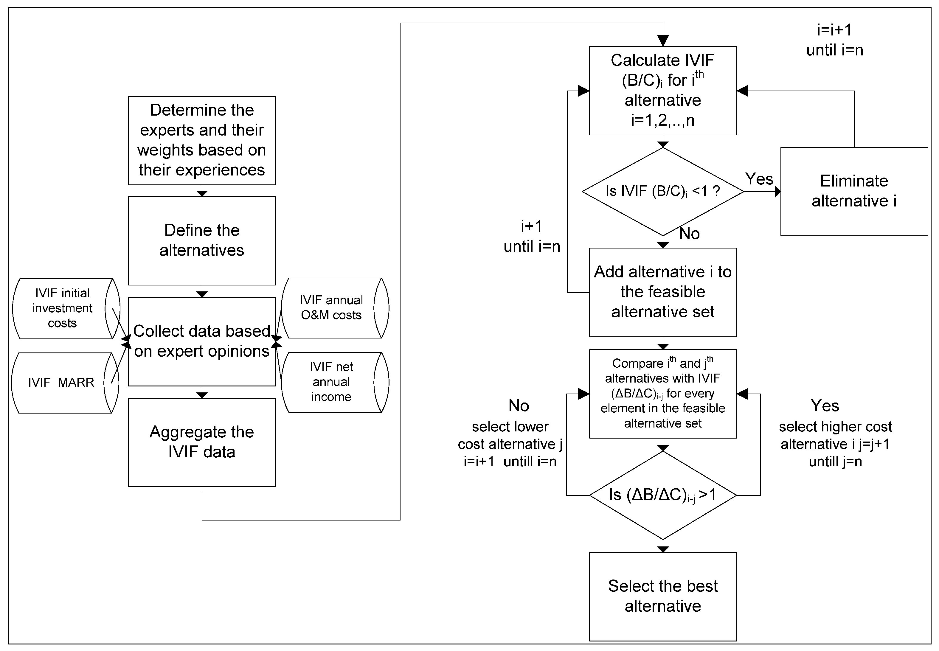
Based on AW terms, B/C ratio for a single alternative is calculated by Equation (29):

$$\frac{\tilde{B}}{\tilde{C}}=\frac{{\widetilde{UAB}}_{Iv, I}}{{\widetilde{FC}}_{Iv, I}\left(\frac{A}{P}, {\tilde{i}}_{Iv, I}, {\tilde{n}}_{Iv, I}\right)+{\widetilde{UAC}}_{Iv, I}-{\widetilde{SV}}_{Iv, I}\left(\frac{A}{F},{\tilde{i}}_{Iv, I},{\tilde{n}}_{Iv, I}\right)}$$

(29)

or

$$\frac{\tilde{B}}{\tilde{C}}=\frac{{\widetilde{UAB}}_{Iv, I}}{{\widetilde{FC}}_{Iv, I}\left[\frac{{\tilde{i}}_{Iv, I}{\left(1+{\tilde{i}}_{Iv, I}\right)}^{{\tilde{n}}_{Iv, I}}}{{\left(1+{\tilde{i}}_{Iv, I}\right)}^{{\tilde{n}}_{Iv, I}}-1}\right]+{\widetilde{UAC}}_{Iv, I}-{\widetilde{SV}}_{Iv, I}\left[\frac{{\tilde{i}}_{Iv, I}}{{\left(1+{\tilde{i}}_{Iv, I}\right)}^{{\tilde{n}}_{Iv, I}}-1}\right]}$$

(30)

Incremental AW-based B/C analysis can be realized by using Equation (31) or Equation (32), assuming crisp and equal lives for the alternatives:

$$\frac{\widetilde{\Delta B}}{\widetilde{\Delta C}}=\frac{{\widetilde{\Delta UAB}}_{Iv, I}}{{\widetilde{\Delta FC}}_{Iv, I}\left(\frac{A}{P}, {\tilde{i}}_{Iv, I}, n\right)+{\widetilde{\Delta UAC}}_{Iv, I}-{\widetilde{\Delta SV}}_{Iv, I}\left(\frac{A}{F},{\tilde{i}}_{Iv, I},n\right)}$$

(31)

or

$$\frac{\widetilde{\Delta B}}{\Delta \tilde{C}}=\frac{{\widetilde{\Delta UAB}}_{Iv, I}}{{\widetilde{\Delta FC}}_{Iv, I}\left[\frac{{\tilde{i}}_{Iv, I}{\left(1+{\tilde{i}}_{Iv, I}\right)}^n}{{\left(1+{\tilde{i}}_{Iv, I}\right)}^n-1}\right]+{\widetilde{\Delta UAC}}_{Iv, I}-{\widetilde{\Delta SV}}_{Iv, I}\left[\frac{{\tilde{i}}_{Iv, I}}{{\left(1+{\tilde{i}}_{Iv, I}\right)}^n-1}\right]}$$

(32)

Incremental B/C analysis would be as follows when assuming intuitionistic fuzzy and unequal lives for the alternatives.

Let ${\tilde{n}}_{Iv,I1}=\left\{n_1,\left[{\mu }_1^{-},{\mu }_1^{+}\right],\left[v_1^{-},v_1^{+}\right]\right\}$ and ${\tilde{n}}_{Iv,I2}=\left\{n_2,\left[{\mu }_2^{-},{\mu }_2^{+}\right],\left[v_2^{-},v_2^{+}\right]\right\}$ be IVIF lives of Alternatives 1 and 2, respectively. Since the IVIF AW analysis will not require a LCML of alternative lives, you can use the own life of each alternative in the calculation as in Equation (33).

(33)

or

(34)

5. Application

In the Marmara Region of Turkey, for an area convenient to wind energy production, a selection among the possible wind energy technology alternatives will be realized. The following three wind energy technologies were evaluated by hesitant and intuitionistic fuzzy sets: E70 2.3MW, E82 3MW, and V112 3.3MW. Each alternative has a useful life of 20 years.

5.1. Crisp Solution

Annual energy production is 111,410,000 kWh for E70 2.3MW wind turbine, 102,300,000 kWh for E82 3MW wind turbine, and 131,600,000 for V112 3.3MW wind turbine.

Table 3 presents the initial investment costs of these alternatives in 2015.

Table 3. Initial investment costs.

	E70 2.3MW wind turbine × 13 units	E82 3MW wind turbine × 10 units	V112 3.3MW wind turbine × 9 units
Turbine costs, $	22,672,000	25,070,000	28,449,000
Foundation costs, $	3,270,000	3,270,000	3,270,000
Connection to the system, $	3,815,000	3,815,000	3,815,000
Planning and license costs, $	3,270,000	3,270,000	3,270,000
Initial Investment cost, $	33,027,000	35,425,000	38,804,000

Table 3. Initial investment costs.

	E70 2.3MW wind turbine × 13 units	E82 3MW wind turbine × 10 units	V112 3.3MW wind turbine × 9 units
Turbine costs, $	22,672,000	25,070,000	28,449,000
Foundation costs, $	3,270,000	3,270,000	3,270,000
Connection to the system, $	3,815,000	3,815,000	3,815,000
Planning and license costs, $	3,270,000	3,270,000	3,270,000
Initial Investment cost, $	33,027,000	35,425,000	38,804,000

The annual maintenance costs between 0–5; 5–10; 10+ years are different since maintenance cost per kWh is $0.019 for the first 5 years, $0.021 for the second 5 years, and $0.025 thereafter. Table 4 shows the annual operating and maintenance costs of the wind energy technology alternatives.

Table 4. Annual operating and maintenance costs, $.

Years	E70 2.3MW wind turbine × 13 units	E82 3MW wind turbine × 10 units	V112 3.3MW wind turbine × 9 units
2016–2020	3,411,993	2,940,010	3,528,679
2021–2025	3,634,813	3,144,610	3,923,479
2026–2035	4,080,453	3,553,810	4,449,879

Table 4. Annual operating and maintenance costs, $.

Years	E70 2.3MW wind turbine × 13 units	E82 3MW wind turbine × 10 units	V112 3.3MW wind turbine × 9 units
2016–2020	3,411,993	2,940,010	3,528,679
2021–2025	3,634,813	3,144,610	3,923,479
2026–2035	4,080,453	3,553,810	4,449,879

Table 5 shows the net annual incomes of the three wind energy alternatives. The annual incomes change after the first 5 years since the feed-in tariff is $0.081 / kWh for the first 5 years and $0.073 / kWh thereafter.

Table 5. Gross and net annual incomes, $.

	E70 2.3MW wind turbine × 13 units		E82 3MW wind turbine × 10 units		V112 3.3MW wind turbine × 9 units
	Gross	Net	Gross	Net	Gross	Net
2016–2020	9,024,210	5,612,217	8,286,300	5,346,290	10,659,600	7,130,921
2021–2025	8,132,930	4,498,117	7,467,900	4,323,290	9,606,800	5,683,321
2026–2035	8,132,930	4,052,477	7,467,900	3,914,090	9,606,800	5,156,921

Table 5. Gross and net annual incomes, $.

	E70 2.3MW wind turbine × 13 units		E82 3MW wind turbine × 10 units		V112 3.3MW wind turbine × 9 units
	Gross	Net	Gross	Net	Gross	Net
2016–2020	9,024,210	5,612,217	8,286,300	5,346,290	10,659,600	7,130,921
2021–2025	8,132,930	4,498,117	7,467,900	4,323,290	9,606,800	5,683,321
2026–2035	8,132,930	4,052,477	7,467,900	3,914,090	9,606,800	5,156,921

Table 6 gives the net present worth (NPW) results of the wind energy technology alternatives based on a minimum attractive rate of return (MARR) of 7.5%, compounded annually.

Because of the space constraints, only the calculations for E70 2.3MW wind turbine are given below.

$$\begin{array}{ll}NP{W}_{E70}& =5,612,217\left(\frac{P}{A},7.5\%,5\right)+4,498,117\left(\frac{P}{A},7.5\%,5\right)\left(\frac{P}{F},7.5\%,5\right)\\ & \hspace{1em}\hspace{1em}\hspace{1em}\hspace{1em}+4,052,477\left(\frac{P}{A},7.5\%,10\right)\left(\frac{P}{F},7.5\%,10\right)-33,027,000\\ & \hspace{1em}\hspace{1em}\hspace{1em}\hspace{1em}=\$15,852,372\end{array}$$

and

Table 6 also gives the B/C results of the three alternatives. All the alternatives are economically feasible. The wind energy turbine V112 3.3MW is the preferred alternative since it has the largest NPW value.

Table 6. NPWs and B/C ratios of the wind energy technology alternatives.

	E70 2.3MW wind turbine × 13 units	E82 3MW wind turbine × 10 units	V112 3.3MW wind turbine × 9 units
NPW, $	15,852,372	11,424,879	23,238,262
B/C	1.224332	1.167969	1.29431

Table 6. NPWs and B/C ratios of the wind energy technology alternatives.

	E70 2.3MW wind turbine × 13 units	E82 3MW wind turbine × 10 units	V112 3.3MW wind turbine × 9 units
NPW, $	15,852,372	11,424,879	23,238,262
B/C	1.224332	1.167969	1.29431

Table 7 selects the best alternative based on incremental B/C ratio analysis. V112 3.3MW is the best alternative since $\Delta B/\Delta C$ ratio between V112 and E70 is larger than 1.0.

Table 7. Incremental B/C ratio analysis.

	$\Delta \mathit{B}/\Delta \mathit{C}$	Decision
E70 vs. E82	2.6726363	Select E70
V112 vs. E70	1.8906222	Select V112

Table 7. Incremental B/C ratio analysis.

	$\Delta \mathit{B}/\Delta \mathit{C}$	Decision
E70 vs. E82	2.6726363	Select E70
V112 vs. E70	1.8906222	Select V112

5.2. Intuitionistic Fuzzy Solution

Although the parameters in Section 5.1 are given by single values, these values can not be known with certainty in reality. For instance, the annual operating and maintenance cost for E70 2.3MW wind turbine between 2016 and 2020 is projected as 3,411,993, even though it can not be forecasted so sharply. Because of the uncertainty of the future, this cost should be defined by an interval. To receive their evaluations under uncertainty and hesitancy, three experts were employed. The experts whose weights are 0.4, 0.4, and 0.2 assigned the intuitionistic fuzzy sets to the investment parameters as follows:

The forecasts for initial investment costs and aggregated IVIFS are presented in Table 8.

Table 8. Aggregated IVIF initial investment costs.

	Possible initial investment costs	IVIFS assigned by three experts	Aggregated IVIFS
E70 2.3MW	$28,000,000	([0.6, 0.9], [0.0, 0.1]), ([0.6, 0.7], [0.1, 0.3]), ([0.5, 0.8], [0.1, 0.2])	([0.5817, 0.8217], [0.0000, 0.1783])
	$30,000,000	([0.5, 0.7],[0.1, 0.2]), ([0.7, 0.8], [0.0, 0.2]), ([0.6, 0.8], [0.0, 0.1]),	([0.6102, 0.7648], [0.0000, 0.1741])
	$32,000,000	([0.7, 0.9], [0.0, 0.1]), ([0.5, 0.8], [0.0, 0.1]), ([0.6, 0.8],[0.0, 0.1])	([0.6102, 0.8484], [0.0000, 0.1000])
E82 3MW	$27,000,000	([0.7, 0.9], [0.0, 0.1]), ([0.6, 0.8], [0.0, 0.2]), ([0.7, 0.8], [0.1, 0.2])	([0.6634, 0.8484], [0.0000, 0.1516])
	$29,000,000	([0.7, 0.8],[0.0, 0.1]), ([0.7, 0.8], [0.1, 0.2]), ([0.6, 0.8], [0.1, 0.2])	([0.6822, 0.8000], [0.0000, 0.1516])
	$31,000,000	([0.6, 0.7], [0.2, 0.3]), ([0.6, 0.8], [0.0, 0.1]), ([0.6, 0.9], [0.0, 0.1])	([0.6000, 0.7952], [0.0000, 0.1552])
V112 3.3MW	$35,000,000	([0.5, 0.7], [0.0, 0.3]), ([0.5, 0.7], [0.1, 0.2]), ([0.5, 0.7],[0.1, 0.3])	([0.5000, 0.7000], [0.0000, 0.2551])
	$36,000,000	([0.7, 0.8], [0.0, 0.1]), ([0.6, 0.9], [0.0, 0.2]), ([0.6, 0.8], [0.1, 0.2])	([0.6435, 0.8484], [0.0000, 0.1516])
	$37,000,000	([0.5, 0.7], [0.2, 0.3]), ([0.7, 0.9], [0.0, 0.1]), ([0.6, 0.9], [0.0, 0.1])	([0.6102, 0.8448], [0.0000, 0.1552])

Table 8. Aggregated IVIF initial investment costs.

	Possible initial investment costs	IVIFS assigned by three experts	Aggregated IVIFS
E70 2.3MW	$28,000,000	([0.6, 0.9], [0.0, 0.1]), ([0.6, 0.7], [0.1, 0.3]), ([0.5, 0.8], [0.1, 0.2])	([0.5817, 0.8217], [0.0000, 0.1783])
	$30,000,000	([0.5, 0.7],[0.1, 0.2]), ([0.7, 0.8], [0.0, 0.2]), ([0.6, 0.8], [0.0, 0.1]),	([0.6102, 0.7648], [0.0000, 0.1741])
	$32,000,000	([0.7, 0.9], [0.0, 0.1]), ([0.5, 0.8], [0.0, 0.1]), ([0.6, 0.8],[0.0, 0.1])	([0.6102, 0.8484], [0.0000, 0.1000])
E82 3MW	$27,000,000	([0.7, 0.9], [0.0, 0.1]), ([0.6, 0.8], [0.0, 0.2]), ([0.7, 0.8], [0.1, 0.2])	([0.6634, 0.8484], [0.0000, 0.1516])
	$29,000,000	([0.7, 0.8],[0.0, 0.1]), ([0.7, 0.8], [0.1, 0.2]), ([0.6, 0.8], [0.1, 0.2])	([0.6822, 0.8000], [0.0000, 0.1516])
	$31,000,000	([0.6, 0.7], [0.2, 0.3]), ([0.6, 0.8], [0.0, 0.1]), ([0.6, 0.9], [0.0, 0.1])	([0.6000, 0.7952], [0.0000, 0.1552])
V112 3.3MW	$35,000,000	([0.5, 0.7], [0.0, 0.3]), ([0.5, 0.7], [0.1, 0.2]), ([0.5, 0.7],[0.1, 0.3])	([0.5000, 0.7000], [0.0000, 0.2551])
	$36,000,000	([0.7, 0.8], [0.0, 0.1]), ([0.6, 0.9], [0.0, 0.2]), ([0.6, 0.8], [0.1, 0.2])	([0.6435, 0.8484], [0.0000, 0.1516])
	$37,000,000	([0.5, 0.7], [0.2, 0.3]), ([0.7, 0.9], [0.0, 0.1]), ([0.6, 0.9], [0.0, 0.1])	([0.6102, 0.8448], [0.0000, 0.1552])

Table 9 shows the IVIF annual operating and maintenance costs of the wind energy technology alternatives.

Table 9. Annual operating and maintenance costs, $.

Years	E70 2.3MW wind turbine × 13 units		E82 3MW wind turbine × 10 units		V112 3.3MW wind turbine × 9 units
2016–2020	3,300,000	([0.7, 0.9], [0.0, 0.1]); ([0.6, 0.8], [0.1, 0.2]); ([0.7, 0.8], [0.1, 0.2])	2,900,000	([0.7, 0.8], [0.0, 0.2]); ([0.5, 0.9], [0.0, 0.1]); ([0.5, 0.8], [0.1, 0.2])	3,400,000	([0.6, 0.8], [0.0, 0.1]) ; ([0.6, 0.9], [0.0, 0.1]); ([0.7, 0.8], [0.1, 0.2])
	3,400,000	([0.7, 0.8], [0.0, 0.1]); ([0.7, 0.8], [0.1, 0.2]); ([0.6, 0.8], [0.1, 0.2])	3,000,000	([0.6, 0.9], [0.0, 0.1]); ([0.6, 0.7], [0.0, 0.2]); ([0.6, 0.8], [0.0, 0.1])	3,500,000	([0.6, 0.7], [0.0, 0.2]) ; ([0.5, 0.8], [0.1, 0.2]); ([0.6, 0.8], [0.0, 0.2])
	3,500,000	([0.7, 0.9], [0.0, 0.1]); ([0.6, 0.7], [0.1, 0.2]); ([0.6, 0.8], [0.0, 0.1])	3,100,000	([0.6, 0.7], [0.0, 0.2]) ; ([0.5, 0.8], [0.1, 0.2]); ([0.6, 0.8], [0.0, 0.2])	3,600,000	([0.7, 0.8], [0.0, 0.1]); ([0.7, 0.8], [0.1, 0.2]); ([0.6, 0.8], [0.1, 0.2])
2021–2025	3,500,000	([0.6, 0.8], [0.1, 0.2]); ([0.7, 0.8], [0.0, 0.1]); ([0.6, 0.9], [0.0, 0.1])	3,000,000	([0.6, 0.8], [0.1, 0.2]); ([0.6, 0.7], [0.0, 0.3]); ([0.5, 0.6], [0.2, 0.3])	3,900,000	([0.5, 0.6], [0.0, 0.3]); ([0.7, 0.9], [0.0, 0.1]); ([0.6, 0.8], [0.0, 0.2])
	3,600,000	([0.7, 0.8], [0.0, 0.2]); ([0.6, 0.7], [0.1, 0.3]); ([0.5, 0.7], [0.2, 0.3])	3,100,000	([0.6, 0.7], [0.1, 0.2]); ([0.7, 0.9], [0.0, 0.1]); ([0.6, 0.7], [0.0, 0.1])	4,000,000	([0.7, 0.8], [0.1, 0.2]); ([0.7, 0.8], [0.0, 0.2]); ([0.7, 0.9], [0.0, 0.1])
	3,700,000	([0.6, 0.8], [0.0, 0.1]); ([0.5, 0.7], [0.0, 0.1]); ([0.5, 0.8], [0.0, 0.1])	3,200,000	([0.6, 0.9], [0.0, 0.1]); ([0.6, 0.8], [0.0, 0.2]); ([0.5, 0.8], [0.1, 0.2])	4,100,000	([0.6, 0.9], [0.0, 0.1]); ([0.7, 0.8], [0.0, 0.1]); ([0.7, 0.9], [0.0, 0.1])
2026–2035	3,900,000	([0.6, 0.8], [0.0, 0.1]); ([0.7, 0.8], [0.0, 0.2]); ([0.5, 0.8], [0.0, 0.2])	3,500,000	([0.7, 0.8], [0.0, 0.2]); ([0.5, 0.8], [0.0, 0.1]); ([0.5, 0.9], [0.0, 0.1])	3,500,000	([0.8, 0.9], [0.0, 0.1]); ([0.7, 0.8], [0.0, 0.2]); ([0.6, 0.9], [0.0, 0.1])
	4,000,000	([0.7, 0.8], [0.1, 0.2]); ([0.5, 0.8], [0.0, 0.2]); ([0.6, 0.8], [0.0, 0.1])	3,600,000	([0.7, 0.8], [0.0, 0.1]); ([0.7, 0.8], [0.1, 0.2]); ([0.6, 0.8], [0.0, 0.2])	4,000,000	([0.5, 0.8], [0.0, 0.1]); ([0.6, 0.8], [0.0, 0.1]); ([0.7, 0.8], [0.0, 0.1])
	4,100,000	([0.7, 0.8], [0.0, 0.1]); ([0.5, 0.6], [0.0, 0.3]); ([0.5, 0.8], [0.0, 0.1])	3,700,000	([0.5, 0.8], [0.0, 0.2]); ([0.6, 0.8], [0.0, 0.2]); ([0.5, 0.7], [0.0, 0.2])	4,500,000	([0.7, 0.8], [0.0, 0.1]); ([0.6, 0.8], [0.0, 0.2]); ([0.5, 0.7], [0.0, 0.1])

Table 9. Annual operating and maintenance costs, $.

Years	E70 2.3MW wind turbine × 13 units		E82 3MW wind turbine × 10 units		V112 3.3MW wind turbine × 9 units
2016–2020	3,300,000	([0.7, 0.9], [0.0, 0.1]); ([0.6, 0.8], [0.1, 0.2]); ([0.7, 0.8], [0.1, 0.2])	2,900,000	([0.7, 0.8], [0.0, 0.2]); ([0.5, 0.9], [0.0, 0.1]); ([0.5, 0.8], [0.1, 0.2])	3,400,000	([0.6, 0.8], [0.0, 0.1]) ; ([0.6, 0.9], [0.0, 0.1]); ([0.7, 0.8], [0.1, 0.2])
	3,400,000	([0.7, 0.8], [0.0, 0.1]); ([0.7, 0.8], [0.1, 0.2]); ([0.6, 0.8], [0.1, 0.2])	3,000,000	([0.6, 0.9], [0.0, 0.1]); ([0.6, 0.7], [0.0, 0.2]); ([0.6, 0.8], [0.0, 0.1])	3,500,000	([0.6, 0.7], [0.0, 0.2]) ; ([0.5, 0.8], [0.1, 0.2]); ([0.6, 0.8], [0.0, 0.2])
	3,500,000	([0.7, 0.9], [0.0, 0.1]); ([0.6, 0.7], [0.1, 0.2]); ([0.6, 0.8], [0.0, 0.1])	3,100,000	([0.6, 0.7], [0.0, 0.2]) ; ([0.5, 0.8], [0.1, 0.2]); ([0.6, 0.8], [0.0, 0.2])	3,600,000	([0.7, 0.8], [0.0, 0.1]); ([0.7, 0.8], [0.1, 0.2]); ([0.6, 0.8], [0.1, 0.2])
2021–2025	3,500,000	([0.6, 0.8], [0.1, 0.2]); ([0.7, 0.8], [0.0, 0.1]); ([0.6, 0.9], [0.0, 0.1])	3,000,000	([0.6, 0.8], [0.1, 0.2]); ([0.6, 0.7], [0.0, 0.3]); ([0.5, 0.6], [0.2, 0.3])	3,900,000	([0.5, 0.6], [0.0, 0.3]); ([0.7, 0.9], [0.0, 0.1]); ([0.6, 0.8], [0.0, 0.2])
	3,600,000	([0.7, 0.8], [0.0, 0.2]); ([0.6, 0.7], [0.1, 0.3]); ([0.5, 0.7], [0.2, 0.3])	3,100,000	([0.6, 0.7], [0.1, 0.2]); ([0.7, 0.9], [0.0, 0.1]); ([0.6, 0.7], [0.0, 0.1])	4,000,000	([0.7, 0.8], [0.1, 0.2]); ([0.7, 0.8], [0.0, 0.2]); ([0.7, 0.9], [0.0, 0.1])
	3,700,000	([0.6, 0.8], [0.0, 0.1]); ([0.5, 0.7], [0.0, 0.1]); ([0.5, 0.8], [0.0, 0.1])	3,200,000	([0.6, 0.9], [0.0, 0.1]); ([0.6, 0.8], [0.0, 0.2]); ([0.5, 0.8], [0.1, 0.2])	4,100,000	([0.6, 0.9], [0.0, 0.1]); ([0.7, 0.8], [0.0, 0.1]); ([0.7, 0.9], [0.0, 0.1])
2026–2035	3,900,000	([0.6, 0.8], [0.0, 0.1]); ([0.7, 0.8], [0.0, 0.2]); ([0.5, 0.8], [0.0, 0.2])	3,500,000	([0.7, 0.8], [0.0, 0.2]); ([0.5, 0.8], [0.0, 0.1]); ([0.5, 0.9], [0.0, 0.1])	3,500,000	([0.8, 0.9], [0.0, 0.1]); ([0.7, 0.8], [0.0, 0.2]); ([0.6, 0.9], [0.0, 0.1])
	4,000,000	([0.7, 0.8], [0.1, 0.2]); ([0.5, 0.8], [0.0, 0.2]); ([0.6, 0.8], [0.0, 0.1])	3,600,000	([0.7, 0.8], [0.0, 0.1]); ([0.7, 0.8], [0.1, 0.2]); ([0.6, 0.8], [0.0, 0.2])	4,000,000	([0.5, 0.8], [0.0, 0.1]); ([0.6, 0.8], [0.0, 0.1]); ([0.7, 0.8], [0.0, 0.1])
	4,100,000	([0.7, 0.8], [0.0, 0.1]); ([0.5, 0.6], [0.0, 0.3]); ([0.5, 0.8], [0.0, 0.1])	3,700,000	([0.5, 0.8], [0.0, 0.2]); ([0.6, 0.8], [0.0, 0.2]); ([0.5, 0.7], [0.0, 0.2])	4,500,000	([0.7, 0.8], [0.0, 0.1]); ([0.6, 0.8], [0.0, 0.2]); ([0.5, 0.7], [0.0, 0.1])

Table 10 presents the aggregated IVIF annual operating and maintenance costs.

Table 10. Aggregated IVIF annual operating and maintenance costs.

Years	E70 2.3MW wind turbine × 13 units		E82 3MW wind turbine × 10 units		V112 3.3MW wind turbine × 9 units
2016–2020	3,300,000	([0.6634, 0.8484], [0.0000, 0.1516])	2,900,000	([0.5924, 0.8484], [0.0000, 0,1596])	3,400,000	([0.6224, 0.8484], [0.0000, 0.1149])
	3,400,000	([0.6822, 0.8000], [0.0000, 0.1516])	3,000,000	([0.6000, 0.8217], [0.0000, 0.1320])	3,500,000	([0.5627, 0.7648], [0.0000, 0.2000])
	3,500,000	([0.6435, 0.8217], [0.0000, 0.1516])	3,100,000	([0.5627, 0.7648], [0.0000, 0.2000])	3,600,000	([0.6822, 0.8000], [0.0000, 0.1516])
2021–2025	3,500,000	([0.6435, 0.8259], [0.0000, 0.1320])	3,000,000	([0.5817, 0.7298], [0.0000, 0.2000])	3,900,000	([0.6822, 0.8000], [0.0000, 0.1516])
	3,600,000	([0.7788, 07449], [0.0000, 0.2551])	3,100,000	([0.6435, 0.8067], [0.0000, 0.1320])	4,000,000	([0.7000, 0.8259], [0.0000, 0.1741])
	3,700,000	([0.5427, 0.7648], [0.0000, 0.1000])	3,200,000	([0.5817, 0.8484], [0.0000, 0.1516])	4,100,000	([0.6634, 0.8680], [0.0000, 0.1000])
2026–2035	3,900,000	([0.6272, 0.8000], [0.0000, 0.1516])	3,500,000	([0.5924, 0.8259], [0.0000, 0.1320])	3,500,000	([0.7298, 0.8680], [0.0000, 0.1320])
	4,000,000	([0.6102, 0.8000], [0.0000, 0.1741])	3,600,000	([0.6282, 0.8000], [0.0000, 0.5116])	4,000,000	([0.5871, 0.8000], [0.0000, 0.1000])
	4,100,000	([0.5924, 0.7361], [0.0000, 0.1552])	3,700,000	([0.5427, 0.7831], [0.0000, 0.2000])	4,500,000	([0.6272, 0.7831], [0.0000, 0.1320])

Table 10. Aggregated IVIF annual operating and maintenance costs.

Years	E70 2.3MW wind turbine × 13 units		E82 3MW wind turbine × 10 units		V112 3.3MW wind turbine × 9 units
2016–2020	3,300,000	([0.6634, 0.8484], [0.0000, 0.1516])	2,900,000	([0.5924, 0.8484], [0.0000, 0,1596])	3,400,000	([0.6224, 0.8484], [0.0000, 0.1149])
	3,400,000	([0.6822, 0.8000], [0.0000, 0.1516])	3,000,000	([0.6000, 0.8217], [0.0000, 0.1320])	3,500,000	([0.5627, 0.7648], [0.0000, 0.2000])
	3,500,000	([0.6435, 0.8217], [0.0000, 0.1516])	3,100,000	([0.5627, 0.7648], [0.0000, 0.2000])	3,600,000	([0.6822, 0.8000], [0.0000, 0.1516])
2021–2025	3,500,000	([0.6435, 0.8259], [0.0000, 0.1320])	3,000,000	([0.5817, 0.7298], [0.0000, 0.2000])	3,900,000	([0.6822, 0.8000], [0.0000, 0.1516])
	3,600,000	([0.7788, 07449], [0.0000, 0.2551])	3,100,000	([0.6435, 0.8067], [0.0000, 0.1320])	4,000,000	([0.7000, 0.8259], [0.0000, 0.1741])
	3,700,000	([0.5427, 0.7648], [0.0000, 0.1000])	3,200,000	([0.5817, 0.8484], [0.0000, 0.1516])	4,100,000	([0.6634, 0.8680], [0.0000, 0.1000])
2026–2035	3,900,000	([0.6272, 0.8000], [0.0000, 0.1516])	3,500,000	([0.5924, 0.8259], [0.0000, 0.1320])	3,500,000	([0.7298, 0.8680], [0.0000, 0.1320])
	4,000,000	([0.6102, 0.8000], [0.0000, 0.1741])	3,600,000	([0.6282, 0.8000], [0.0000, 0.5116])	4,000,000	([0.5871, 0.8000], [0.0000, 0.1000])
	4,100,000	([0.5924, 0.7361], [0.0000, 0.1552])	3,700,000	([0.5427, 0.7831], [0.0000, 0.2000])	4,500,000	([0.6272, 0.7831], [0.0000, 0.1320])

Table 11 shows the IVIF net annual incomes of the three wind energy alternatives and their aggregated IVIF values. The feed-in tariff is still crisp since it is informed by the government when you decide to invest.

Table 11. IVIF net annual incomes, $.

Years	E70 2.3MW wind turbine × 13 units		Aggregated IVIFS	E82 3MW wind turbine × 10 units		Aggregated IVIFS	V112 3.3MW wind turbine × 9 units		Aggregated IVIFS
2016–2020	8,500,000	([0.7, 0.9], [0.0, 0.1]); ([0.6, 0.8], [0.1, 0.2]); ([0.7, 0.8], [0.1, 0.2])	([0.6634, 0.8484], [0.0000, 0.1516])	8,000,000	([0.7, 0.8], [0.0, 0.2]); ([0.5, 0.9], [0.0, 0.1]); ([0.5, 0.8], [0.1, 0.2])	([0.5924, 0.8484], [0.0000, 0.1516])	10,000,000	([0.6, 0.8], [0.0, 0.1]) ; ([0.6, 0.9], [0.0, 0.1]); ([0.7, 0.8], [0.1, 0.2])	([0.6224, 0.8484], [0.0000, 0.1149])
	9,000,000	([0.7, 0.8], [0.0, 0.1]); ([0.7, 0.8], [0.1, 0.2]); ([0.6, 0.8], [0.1, 0.2])	([0.6822, 0.8000], [0.0000, 0.1516])	8,250,000	([0.6, 0.9], [0.0, 0.1]); ([0.6, 0.7], [0.0, 0.2]); ([0.6, 0.8], [0.0, 0.1])	([0.6000, 0.8217], [0.0000, 0.1320])	10,500,000	([0.6, 0.7], [0.0, 0.2]) ; ([0.5, 0.8], [0.1, 0.2]); ([0.6, 0.8], [0.0, 0.2])	([0.5627, 0.7648], [0.0000, 0.2000])
	9,500,000	([0.7, 0.9], [0.0, 0.1]); ([0.6, 0.7], [0.1, 0.2]); ([0.6, 0.8], [0.0, 0.1])	([0.6435, 0.8217], [0.0000, 0.1320])	8,500,000	([0.6, 0.7], [0.0, 0.2]) ; ([0.5, 0.8], [0.1, 0.2]); ([0.6, 0.8], [0.0, 0.2])	([0.5627, 0.7648], [0.0000, 0.2000])	11,000,000	([0.7, 0.8], [0.0, 0.1]); ([0.7, 0.8], [0.1, 0.2]); ([0.6, 0.8], [0.1, 0.2])	([0.6822, 0.8000], [0.0000, 0.1516])
2021–2025	7,500,000	([0.6, 0.8], [0.1, 0.2]); ([0.7, 0.8], [0.0, 0.1]); ([0.6, 0.9], [0.0, 0.1])	([0.6435, 0.8259], [0.0000, 0.2551])	7,000,000	([0.6, 0.8], [0.1, 0.2]); ([0.6, 0.7], [0.0, 0.3]); ([0.5, 0.6], [0.2, 0.3])	([0.6435, 0.7298], [0.0000, 0.2551])	9,000,000	([0.5, 0.6], [0.0, 0.3]); ([0.7, 0.9], [0.0, 0.1]); ([0.6, 0.8], [0.0, 0.2])	([0.6102, 0.8000], [0.0000, 0.1783])
	8,000,000	([0.7, 0.8], [0.0, 0.2]); ([0.6, 0.7], [0.1, 0.3]); ([0.5, 0.7], [0.2, 0.3])	([0.6272, 0.7449], [0.0000, 0.2551])	7,500,000	([0.6, 0.7], [0.1, 0.2]); ([0.7, 0.9], [0.0, 0.1]); ([0.6, 0.7], [0.0, 0.1])	([0.6435, 0.8067], [0.0000, 0.1320])	9,500,000	([0.7, 0.8], [0.1, 0.2]); ([0.7, 0.8], [0.0, 0.2]); ([0.7, 0.9], [0.0, 0.1])	([0.7000, 0.8259], [0.0000, 0.1741])
	8,500,000	([0.6, 0.8], [0.0, 0.1]); ([0.5, 0.7], [0.0, 0.1]); ([0.5, 0.8], [0.0, 0.1])	([0.5427, 0.7648], [0.0000, 0.1000])	8,000,000	([0.6, 0.9], [0.0, 0.1]); ([0.6, 0.8], [0.0, 0.2]); ([0.5, 0.8], [0.1, 0.2])	([0.5817, 0.8484], [0.0000, 0.1516])	10,000,000	([0.6, 0.9], [0.0, 0.1]); ([0.7, 0.8], [0.0, 0.1]); ([0.7, 0.9], [0.0, 0.1])	([0.6634, 0.8680], [0.0000, 0.1000])
2026–2035	7,500,000	([0.6, 0.8], [0.0, 0.1]); ([0.7, 0.8], [0.0, 0.2]); ([0.5, 0.8], [0.0, 0.2])	([0.6272, 0.7648], [0.0000, 0.1000])	7,000,000	([0.7, 0.8], [0.0, 0.2]); ([0.5, 0.8], [0.0, 0.1]); ([0.5, 0.9], [0.0, 0.1])	([0.5817, 0.8484], [0.0000, 0.1516])	9,000,000	([0.8, 0.9], [0.0, 0.1]); ([0.7, 0.8], [0.0, 0.2]); ([0.6, 0.9], [0.0, 0.1])	([0.6634, 0.8680], [0.0000, 0.1320])
	8,000,000	([0.7, 0.8], [0.1, 0.2]); ([0.5, 0.8], [0.0, 0.2]); ([0.6, 0.8], [0.0, 0.1])	([0.6102, 0.8000], [0.0000, 0.1741])	7,500,000	([0.7, 0.8], [0.0, 0.1]); ([0.7, 0.8], [0.1, 0.2]); ([0.6, 0.8], [0.0, 0.2])	([0.6822, 0.8000], [0.0000, 0.1516])	9,500,000	([0.5, 0.8], [0.0, 0.1]); ([0.6, 0.8], [0.0, 0.1]); ([0.7, 0.8], [0.0, 0.1])	([0.5871, 0.8000], [0.0000, 0.1000])
	8,500,000	([0.7, 0.8], [0.0, 0.1]); ([0.5, 0.6], [0.0, 0.3]); ([0.5, 0.8], [0.0, 0.1])	([0.6634, 0.8484], [0.0000, 0.1516])	8,000,000	([0.5, 0.8], [0.0, 0.2]); ([0.6, 0.8], [0.0, 0.2]); ([0.5, 0.7], [0.0, 0.2])	([0.5427, 0.7831], [0.0000, 0.2000])	10,000,000	([0.7, 0.8], [0.0, 0.1]); ([0.6, 0.8], [0.0, 0.2]); ([0.5, 0.7], [0.0, 0.1])	([0.6272, 0.7831], [0.0000, 0.1320])

Table 11. IVIF net annual incomes, $.

Years	E70 2.3MW wind turbine × 13 units		Aggregated IVIFS	E82 3MW wind turbine × 10 units		Aggregated IVIFS	V112 3.3MW wind turbine × 9 units		Aggregated IVIFS
2016–2020	8,500,000	([0.7, 0.9], [0.0, 0.1]); ([0.6, 0.8], [0.1, 0.2]); ([0.7, 0.8], [0.1, 0.2])	([0.6634, 0.8484], [0.0000, 0.1516])	8,000,000	([0.7, 0.8], [0.0, 0.2]); ([0.5, 0.9], [0.0, 0.1]); ([0.5, 0.8], [0.1, 0.2])	([0.5924, 0.8484], [0.0000, 0.1516])	10,000,000	([0.6, 0.8], [0.0, 0.1]) ; ([0.6, 0.9], [0.0, 0.1]); ([0.7, 0.8], [0.1, 0.2])	([0.6224, 0.8484], [0.0000, 0.1149])
	9,000,000	([0.7, 0.8], [0.0, 0.1]); ([0.7, 0.8], [0.1, 0.2]); ([0.6, 0.8], [0.1, 0.2])	([0.6822, 0.8000], [0.0000, 0.1516])	8,250,000	([0.6, 0.9], [0.0, 0.1]); ([0.6, 0.7], [0.0, 0.2]); ([0.6, 0.8], [0.0, 0.1])	([0.6000, 0.8217], [0.0000, 0.1320])	10,500,000	([0.6, 0.7], [0.0, 0.2]) ; ([0.5, 0.8], [0.1, 0.2]); ([0.6, 0.8], [0.0, 0.2])	([0.5627, 0.7648], [0.0000, 0.2000])
	9,500,000	([0.7, 0.9], [0.0, 0.1]); ([0.6, 0.7], [0.1, 0.2]); ([0.6, 0.8], [0.0, 0.1])	([0.6435, 0.8217], [0.0000, 0.1320])	8,500,000	([0.6, 0.7], [0.0, 0.2]) ; ([0.5, 0.8], [0.1, 0.2]); ([0.6, 0.8], [0.0, 0.2])	([0.5627, 0.7648], [0.0000, 0.2000])	11,000,000	([0.7, 0.8], [0.0, 0.1]); ([0.7, 0.8], [0.1, 0.2]); ([0.6, 0.8], [0.1, 0.2])	([0.6822, 0.8000], [0.0000, 0.1516])
2021–2025	7,500,000	([0.6, 0.8], [0.1, 0.2]); ([0.7, 0.8], [0.0, 0.1]); ([0.6, 0.9], [0.0, 0.1])	([0.6435, 0.8259], [0.0000, 0.2551])	7,000,000	([0.6, 0.8], [0.1, 0.2]); ([0.6, 0.7], [0.0, 0.3]); ([0.5, 0.6], [0.2, 0.3])	([0.6435, 0.7298], [0.0000, 0.2551])	9,000,000	([0.5, 0.6], [0.0, 0.3]); ([0.7, 0.9], [0.0, 0.1]); ([0.6, 0.8], [0.0, 0.2])	([0.6102, 0.8000], [0.0000, 0.1783])
	8,000,000	([0.7, 0.8], [0.0, 0.2]); ([0.6, 0.7], [0.1, 0.3]); ([0.5, 0.7], [0.2, 0.3])	([0.6272, 0.7449], [0.0000, 0.2551])	7,500,000	([0.6, 0.7], [0.1, 0.2]); ([0.7, 0.9], [0.0, 0.1]); ([0.6, 0.7], [0.0, 0.1])	([0.6435, 0.8067], [0.0000, 0.1320])	9,500,000	([0.7, 0.8], [0.1, 0.2]); ([0.7, 0.8], [0.0, 0.2]); ([0.7, 0.9], [0.0, 0.1])	([0.7000, 0.8259], [0.0000, 0.1741])
	8,500,000	([0.6, 0.8], [0.0, 0.1]); ([0.5, 0.7], [0.0, 0.1]); ([0.5, 0.8], [0.0, 0.1])	([0.5427, 0.7648], [0.0000, 0.1000])	8,000,000	([0.6, 0.9], [0.0, 0.1]); ([0.6, 0.8], [0.0, 0.2]); ([0.5, 0.8], [0.1, 0.2])	([0.5817, 0.8484], [0.0000, 0.1516])	10,000,000	([0.6, 0.9], [0.0, 0.1]); ([0.7, 0.8], [0.0, 0.1]); ([0.7, 0.9], [0.0, 0.1])	([0.6634, 0.8680], [0.0000, 0.1000])
2026–2035	7,500,000	([0.6, 0.8], [0.0, 0.1]); ([0.7, 0.8], [0.0, 0.2]); ([0.5, 0.8], [0.0, 0.2])	([0.6272, 0.7648], [0.0000, 0.1000])	7,000,000	([0.7, 0.8], [0.0, 0.2]); ([0.5, 0.8], [0.0, 0.1]); ([0.5, 0.9], [0.0, 0.1])	([0.5817, 0.8484], [0.0000, 0.1516])	9,000,000	([0.8, 0.9], [0.0, 0.1]); ([0.7, 0.8], [0.0, 0.2]); ([0.6, 0.9], [0.0, 0.1])	([0.6634, 0.8680], [0.0000, 0.1320])
	8,000,000	([0.7, 0.8], [0.1, 0.2]); ([0.5, 0.8], [0.0, 0.2]); ([0.6, 0.8], [0.0, 0.1])	([0.6102, 0.8000], [0.0000, 0.1741])	7,500,000	([0.7, 0.8], [0.0, 0.1]); ([0.7, 0.8], [0.1, 0.2]); ([0.6, 0.8], [0.0, 0.2])	([0.6822, 0.8000], [0.0000, 0.1516])	9,500,000	([0.5, 0.8], [0.0, 0.1]); ([0.6, 0.8], [0.0, 0.1]); ([0.7, 0.8], [0.0, 0.1])	([0.5871, 0.8000], [0.0000, 0.1000])
	8,500,000	([0.7, 0.8], [0.0, 0.1]); ([0.5, 0.6], [0.0, 0.3]); ([0.5, 0.8], [0.0, 0.1])	([0.6634, 0.8484], [0.0000, 0.1516])	8,000,000	([0.5, 0.8], [0.0, 0.2]); ([0.6, 0.8], [0.0, 0.2]); ([0.5, 0.7], [0.0, 0.2])	([0.5427, 0.7831], [0.0000, 0.2000])	10,000,000	([0.7, 0.8], [0.0, 0.1]); ([0.6, 0.8], [0.0, 0.2]); ([0.5, 0.7], [0.0, 0.1])	([0.6272, 0.7831], [0.0000, 0.1320])

Table 12 presents the aggregated IVIF MARR values. The IVIF B/C and $\Delta B/\Delta C$ ratios will be calculated based on the IVIF MARR.

Table 12. Aggregated and defuzzified IVIF MARR.

Possible MARRs	Membership intervals	Aggregated
7.0%	([0.5, 0.6], [0.2, 0.4]), ([0.6, 0.7], [0.2, 0.3]), ([0.5, 0.6], [0.2, 0.3])	([0.5427, 0.6435], [0.2, 0.3366])
7.5%	([0.7, 0.9], [0.0, 0.1]), ([0.8, 0.9], [0.0, 0.1]), ([0.7, 0.8], [0.0, 0.2])	([0.7449, 0.8851], [0, 0.1149])
8.0%	([0.6, 0.7], [0.2, 0.3]), ([0.7, 0.8], [0.0, 0.2]), ([0.6, 0.7], [0.1, 0.2])	([0.6435, 0.7449], [0, 0.2352])

Table 12. Aggregated and defuzzified IVIF MARR.

Possible MARRs	Membership intervals	Aggregated
7.0%	([0.5, 0.6], [0.2, 0.4]), ([0.6, 0.7], [0.2, 0.3]), ([0.5, 0.6], [0.2, 0.3])	([0.5427, 0.6435], [0.2, 0.3366])
7.5%	([0.7, 0.9], [0.0, 0.1]), ([0.8, 0.9], [0.0, 0.1]), ([0.7, 0.8], [0.0, 0.2])	([0.7449, 0.8851], [0, 0.1149])
8.0%	([0.6, 0.7], [0.2, 0.3]), ([0.7, 0.8], [0.0, 0.2]), ([0.6, 0.7], [0.1, 0.2])	([0.6435, 0.7449], [0, 0.2352])

For 7%, the IVIF sets assigned by three experts are aggregated as follows:

$$\begin{array}{l}([1-(1-0.5{)}^{0.4}\times (1-0.6{)}^{0.4}\times (1-0.5{)}^{0.2},1-(1-0.6{)}^{0.4}\times (1-0.7{)}^{0.4}\times (1-0.6{)}^{0.2}],\\ [{0.2}^{0.4}\times {0.2}^{0.4}\times {0.2}^{0.2},{0.4}^{0.4}\times {0.3}^{0.4}\times {0.3}^{0.2}])=([0.5427,0.6435],[0.2,0.3366])\end{array}$$

We now apply the arithmetic operations given in Section 3.1. The following calculations are realized for E70, E82, and V112, respectively:

For E70:

Using the arithmetic operations of IVIFS given by Equation (4)–(10), the B/C ratio is calculated as follows:

In order to clarify the operations, the first term in the numerator and the final result in the above calculation, as an example, is obtained as follows:

$$\langle \left(9,000,000\left(\frac{P}{A},7.5\%,5\right)=36,412,964\right);\left(\left(\left[0.6634, 0.8245\right],\left[0, 0.1448\right]\right)\times \left(\left[0.6535, 0.7814\right],\left[0, 0.2087\right]\right)=\left(\left[0.6634\times 0.6535,0.8245\times 0.7814\right],\left[0, 0.1448+0.2087-0.1448\times 0.2087\right]\right)=\left(\left[0.4335,0.6443\right],\left[0,0.3233\right]\right)\right)\rangle$$

The final result is obtained as follows:

$$\langle \left(\frac{85,601,816}{67,223,156}=1.2734\right);\left(\left(\left[\min \left(0.6897,0.8806\right),\min \left(0.9013,0.9820\right)\right],\left[\max \left(0,0\right), max\left(0.0731, 0.0106\right)\right]\right)>= \left(\left[0.6897, 0.9013\right],\left[0, 0.0731\right]\right)\right)\rangle$$

NPW can be easily calculated from the equation above by subtracting PWC from PWB such that

$$\begin{gathered} NPW=\langle 85,601,816;\left(\left[0.6897,0.9013\right],\left[0,0.0731\right]\right)\rangle - \langle 67,223,156;\left(\left[0.8806,0.9820\right],\left[0,0.0106\right]\right)\rangle \\ = \langle 18,378,660; \left(\left[0.6897, 0.9013\right],\left[0, 0.0731\right]\right)\rangle \end{gathered}$$

Using Equation (14), the defuzzified value of IVIFS is calculated as 0.7942. The certainty value of NPW for E70 is calculated as $14,596,331.

For E82, the similar operations are applied, and the following result is finally obtained:

$${\left(\frac{B}{C}\right)}_{E82}=\frac{\langle 79,493,099;\left(\left[0.6644, 0.9064\right],\left[0, 0.0770\right]\right)\rangle }{\langle 61,863,540;\left(\left[0.8806, 0.9820\right],\left[0, 0.0106\right]\right)\rangle }=\langle 1.285;\left(\left[0.6644,0.9064\right],\left[0, 0.0770\right]\right)\rangle$$

NPW can be easily calculated from the equation above by subtracting PWC from PWB such that

$$\begin{gathered} NPW=\langle 79,493,099;\left(\left[0.6644,0.9064\right],\left[0,0.0770\right]\right)\rangle - \langle 61,863,540;\left(\left[0.8806,0.9820\right],\left[0,0.0106\right]\right)\rangle \\ = \langle 17,629,559; \left(\left[0.6644,0.9064],[0,0.0770\right]\right)\rangle \end{gathered}$$

Using Equation (14), the defuzzified value of IVIF B/C is calculated as 0.7838. The certainty value of NPW for E82 is calculated as $13,818,048.

For V112, the similar operations are applied and finally the following result is obtained:

$${\left(\frac{B}{C}\right)}_{V112}=\frac{\langle 100,893,553;\left(\left[0.6891, 0.9097\right],\left[0, 0.0687\right]\right)\rangle }{\langle 74,755,022;\left(\left[0.5989, 0.8373\right],\left[0, 0.1356\right]\right)\rangle }=\langle 1.350;\left(\left[0.5989, 0.8373\right],\left[0, 0.1356\right]\right)\rangle$$

NPW can be easily calculated from the equation above by subtracting PWC from PWB such that

$$\begin{gathered} NPW=\langle 100,893,553;\left(\left[0.6891,0.9097\right],\left[0,0.0687\right]\right)\rangle -\langle 74,755,022;\left(\left[0.5989,0.8373\right],\left[0,0.1356\right]\right)\rangle \\ = \langle 26,138,531; \left(\left[0.5989, 0.8373\right],\left[0, 0.1356\right]\right)\rangle \end{gathered}$$

Using Equation (14), the defuzzified value of IVIF B/C ratio is calculated as 0.7181. The certainty value of NPW for V112 is calculated as $18,770,079.

Table 13 summarizes the B/C ratios and NPWs of the alternatives.

Table 13. B/C ratios and NPWs.

Alternatives	B/C ratios	NPWs
E70	$\langle 1.2734; \left(\left[0.6897, 0.9013\right],\left[0, 0.0731\right]\right)\rangle$	$\langle 18,378,660; \left(\left[0.6897, 0.9013\right],\left[0, 0.0731\right]\right)\rangle$
E82	$\langle 1.285;\left(\left[0.6644,0.9064\right],\left[0, 0.0770\right]\right)\rangle$	$\langle 17,629,559; \left(\left[0.6644,0.9064],[0,0.0770\right]\right)\rangle$
V112	$\langle 1.350;\left(\left[0.5989, 0.8373\right],\left[0, 0.1356\right]\right)\rangle$	$\langle 26,138,531; \left(\left[0.5989, 0.8373\right],\left[0, 0.1356\right]\right)\rangle$

Table 13. B/C ratios and NPWs.

Alternatives	B/C ratios	NPWs
E70	$\langle 1.2734; \left(\left[0.6897, 0.9013\right],\left[0, 0.0731\right]\right)\rangle$	$\langle 18,378,660; \left(\left[0.6897, 0.9013\right],\left[0, 0.0731\right]\right)\rangle$
E82	$\langle 1.285;\left(\left[0.6644,0.9064\right],\left[0, 0.0770\right]\right)\rangle$	$\langle 17,629,559; \left(\left[0.6644,0.9064],[0,0.0770\right]\right)\rangle$
V112	$\langle 1.350;\left(\left[0.5989, 0.8373\right],\left[0, 0.1356\right]\right)\rangle$	$\langle 26,138,531; \left(\left[0.5989, 0.8373\right],\left[0, 0.1356\right]\right)\rangle$

Based on NPW analysis, V112 should be selected, since the largest NPW belongs to it. However, B/C analysis requires an incremental analysis when the B/C ratios of alternatives are larger than 1.0.

In our case, all the B/C ratios are larger than 1.0. Hence, an incremental analysis should be made.

For the incremental investment E70-E82, the following calculation is realized.

Using Equation (14), the defuzzified value of IVIFS is calculated as 0.7790. The certainty value of $\Delta$NPW for the increment of “E70 – E82” is calculated as $\left(6,108,717-5,359,616\right)\times 0.7790=$$583,550. Thus, E70 is the selected alternative.

For the incremental investment V112-E70, the similar operations are applied and finally the following result is obtained:

$${\left(\frac{\Delta B}{\Delta C}\right)}_{V112-E70}=\frac{\langle 15,291,737;\left(\left[0.6762, 0.8976\right],\left[0, 0.0744\right]\right)\rangle }{\langle 7,531,867;\left(\left[0.8717, 0,9806\right],\left[0, 0.0132\right]\right)\rangle }=\langle 2.030;\left(\left[0.6762, 0.8976\right],\left[0, 0.0744\right]\right)\rangle$$

Using Equation (14), the defuzzified value of IVIFS is calculated as 0.7861. The certainty value of $\Delta$NPW for the increment of “V112 – E70” is calculated as $6,100,034. Finally, V112 is the selected alternative.

Both the classical B/C analysis and IVIF B/C analysis yielded the same ranking in this real case study. However, since the IVIF B/C analysis involves parameters defined in a more informative and more flexible way, the results from both approaches can be clearly different.

6. Conclusions and Future Research Directions

Environmental sustainability can be provided by making responsible decisions to reduce the negative impacts of these decisions on the environment. It involves both reducing the amount of waste produced or using less energy and developing processes for becoming completely sustainable in the future. Sustainable energy technologies involve renewable energy sources, such as hydroelectricity, solar energy, wind energy, wave power, geothermal energy, bioenergy, and also technologies designed to improve energy efficiency. Wind energy investments as a sustainability project should certainly be based on an economic analysis before making the final decision since more savings support new sustainability projects. Although wind energy investments have been increasing in the last decade, they have not reached their potential due to the falls in fossil fuel prices, uncertainties in the production levels and relatively high initial investment costs of wind energy investments. A comprehensive and flexible representation of investment parameters will clearly increase the sensitivity of the analysis, and more realistic results can be obtained. In this paper, our objective is to provide this kind of economic analysis for wind energy investments that provides environmental sustainability.

We realized the economic analysis of the wind energy technologies based on B/C ratio analysis under fuzziness. Interval-valued intuitionistic fuzzy sets have been used for the B/C ratio comparison among wind energy technologies. IVIF incremental B/C ratio analysis has been developed. We also developed IVIF B/C ratio analysis for the alternatives having different lives. The numerical application showed that the IVIF B/C ratio analysis requires complex calculations with respect to the classical B/C ratio analysis. However, the decision makers can better express their forecasts related to the cash flows of wind energy projects under uncertainty by using fuzzy sets. Intuitionistic fuzzy sets enable decision makers to express their judgments with more details, including their hesitancy. The developed method lets more than one possible value of investment parameters and multiple decision makers be considered in the analysis. Additionally, the membership and non-membership degrees of these parameters can be defined by the decision makers based on their experiences and expectations. Thus, a flexible and more informative approach is provided.

For further research, the cash flow forecasts can be comparatively made by developing hesitant fuzzy B/C ratio analysis or type-2 fuzzy B/C ratio analysis. The same wind energy technologies can be compared by these new B/C ratio analyses.

References

1. Beynaghi, A.; Moztarzadeh, F.; Trencher, G.; Mozafari, M. Energy in sustainability research: A recent rise to prominence. Renew. Sustain. Energy Rev. 2015, 51, 1794–1795. [Google Scholar] [CrossRef]
2. Onar, S.C.; Oztaysi, B.; Otay, I.; Kahraman, C. Multi-expert wind energy technology selection using interval-valued intuitionistic fuzzy sets. Energy 2015, 90, 274–285. [Google Scholar] [CrossRef]
3. GWEC Annual Report 2014. Available online: http://www.gwec.net/publications/global-wind-report-2/global-wind-report-2014-annual-market-update/ (accessed on 19 November 2015).
4. Onar, S.C.; Kilavuz, T.N. Risk analysis of wind energy investments in Turkey. Human Ecol. Risk Assess. 2015, 21, 1230–1245. [Google Scholar] [CrossRef]
5. Ertürk, M. The evaluation of feed-in tariff regulation of Turkey for onshore wind energy based on the economic analysis. Energy Policy 2012, 45, 359–367. [Google Scholar] [CrossRef]
6. Uçar, A.; Balo, F. Assessment of wind power potential for turbine installation in coastal areas of Turkey. Renew. Sustain. Energy Rev. 2010, 14, 1901–1912. [Google Scholar] [CrossRef]
7. Blank, L.T.; Tarquin, J.A. Engineering Economy, 7th ed.; McGraw-Hill Inc.: New York, NY, USA, 2012. [Google Scholar]
8. Zadeh, L.A. Fuzzy Sets. Inf. Control 1989, 8, 338–353. [Google Scholar] [CrossRef]
9. Onar, S.C.; Oztaysi, B.; Kahraman, C. Strategic decision selection using hesitant fuzzy TOPSIS and interval type-2 fuzzy AHP: A case study. Int. J. Comput. İntell. Syst. 2014, 7, 1002–1021. [Google Scholar] [CrossRef]
10. Behret, H.; Öztayşi, B.; Kahraman, C. A fuzzy inference system for supply chain risk management. Pract. Appl. Intell. Syst. 2012. [Google Scholar] [CrossRef]
11. Kaya, I.; Oztaysi, B.; Kahraman, C. A Two-Phased Fuzzy Multicriteria Selection among Public Transportation Investments for Policy-Making and Risk Governance. Int. J. Uncertain. Fuzz. Knowl. Based Syst. 2012. [Google Scholar] [CrossRef]
12. Kahraman, C. Multi-criteria decision-making methods and fuzzy sets. In Fuzzy Multi-Criteria Decision Making: Theory and Applications with Recent Developments; Kahraman, C., Ed.; Springer: New York, NY, USA, 2008; pp. 1–18. [Google Scholar]
13. Zhang, G.; Lu, J. Model and approach of fuzzy bilevel decision-making for logistics planning problem. J. Enterp. Inf. Manag. 2007, 20, 178–197. [Google Scholar]
14. Tüysüz, F.; Kahraman, C. Modeling a flexible manufacturing cell using stochastic Petri nets with fuzzy parameters. Expert Syst. Appl. 2010, 37, 3910–3920. [Google Scholar] [CrossRef]
15. Coban, V.; Onar, S.C.; Soyer, A. Analyzing Dynamic Capabilities via Fuzzy cognitive Maps. Intell. Tech. Eng. Manag. 2015. [Google Scholar] [CrossRef]
16. Oztaysi, B.; Onar, S.C.; Goztepe, K.; Kahraman, C. Evaluation of research proposals for grant funding using interval-valued intuitionistic fuzzy sets. Soft Comput. 2015. [Google Scholar] [CrossRef]
17. Yavuz, M.; Oztaysi, B.; Onar, S.C.; Kahraman, C. Multi-criteria evaluation of alternative-fuel vehicles via a hierarchical hesitant fuzzy linguistic model. Expert Syst. Appl. 2015, 42, 2835–2848. [Google Scholar] [CrossRef]
18. Kahraman, C.; Oztaysi, B.; Onar, S.C. A Multicriteria Supplier Selection Model Using Hesitant Fuzzy Linguistic Term Sets. J. Mult.-Valued Log. Soft Comput. 2015, in press. [Google Scholar]
19. Miyamoto, S. Fuzzy Multisets and Their Generalizations. Lect. Notes Comput. Sci. 2001, 2235, 225–235. [Google Scholar]
20. Kahraman, C.; Oztaysi, B.; Sari, I.U.; Turanoglu, E. Fuzzy analytic hierarchy process with interval type-2 fuzzy sets. Knowl.-Based Syst. 2014, 59, 48–57. [Google Scholar] [CrossRef]
21. Oztaysi, B. A Group Decision Making Approach Using Interval Type-2 Fuzzy AHP for Enterprise Information Systems Project Selection. J. Mult.-Valued Log. Soft Comput. 2015, 24, 475–500. [Google Scholar]
22. Kahraman, C.; Onar, S.C.; Oztaysi, B. Fuzzy Multicriteria Decision-Making: A Literature Review. Int. J. Comput. Intell. Syst. 2015, 8, 637–666. [Google Scholar] [CrossRef]
23. Kahraman, C.; Tolga, E.; Ulukan, Z. Justification of manufacturing technologies using fuzzy benefit-cost ratio analysis. Int. J. Prod. Econ. 2000, 66, 45–52. [Google Scholar] [CrossRef]
24. Herbert, G.M.J.; Sreevalsan, S.I.E.; Rajapandian, S. A review of wind energy technologies. Renew. Sustain. Energy Rev. 2007, 11, 1117–1145. [Google Scholar] [CrossRef]
25. Sarja, J.; Halonen, V. Wind Turbine Selection Criteria: A Customer Perspective. J. Energy Power Eng. 2013, 7, 1795–1802. [Google Scholar]
26. Chowdhury, S.; Zhang, J.; Messac, A.; Castillo, L. Optimizing the arrangement and the selection of turbines for wind farms subject to varying wind conditions. Renew. Energy 2013, 52, 273–282. [Google Scholar] [CrossRef]
27. Perkin, S.; Garrett, D.; Jensson, P. Optimal wind turbine selection methodology: A case-study for Búrfell. Icel. Renew. Energy 2015, 75, 165–172. [Google Scholar] [CrossRef]
28. Mostafaeipour, A.; Jadidi, M.; Mohammadi, K.; Sedaghat, A. An analysis of wind energy potential and economic evaluation in Zahedan, Iran. Renew. Sustain. Energy Rev. 2014, 30, 641–650. [Google Scholar] [CrossRef]
29. Rahimi, S.; Meratizaman, M.; Monadizadeh, S.; Amidpour, M. Techno-economic analysis of wind turbine–PEM (polymer electrolyte membrane) fuel cell hybrid system in standalone area. Energy 2014, 67, 381–396. [Google Scholar] [CrossRef]
30. Schallenberg-Rodriguez, J. A methodological review to estimate techno-economical wind energy production. Renew. Sustain. Energy Rev. 2013, 21, 272–287. [Google Scholar] [CrossRef]
31. Mohammadi, K.; Mostafaeipour, A. Economic feasibility of developing wind turbines in Aligoodarz, Iran. Energy Convers. Manag. 2013, 76, 645–653. [Google Scholar] [CrossRef]
32. EWEA. European Wind Energy Association Report. 2011. Available online: http://www.ewea.org/fileadmin/files/library/publications/reports/EWEA_Annual_Report_2011.pdf (accessed on 19 November 2015).
33. Krohn, S.; Morthorst, P.E.; Awerbuch, S. The Economics of Wind Energy. 2009. Available online: http://www.ewea.org/fileadmin/files/library/publications/reports/Economics_of_Wind_Energy.pdf (accessed on 19 November 2015).
34. Atanassov, K.T. Intuitionistic Fuzzy Sets. Fuzz. Sets Syst. 1986, 20, 87–96. [Google Scholar] [CrossRef]
35. Atanassov, K.T. Intuitionistic Fuzzy Sets: Theory and Applications; Springer: Berlin, Germany, 1999. [Google Scholar]
36. Atanassova, L. On interval-valued intuitionistic fuzzy versions of L. Zadeh's extension principle. Issues Intuit. Fuzzy Sets General. Nets 2008, 7, 13–19. [Google Scholar]
37. Li, D.F. Extension principles for interval-valued intuitionistic fuzzy sets and algebraic operations. Fuzzy Optim. Decis. Mak. 2011, 10, 45–48. [Google Scholar] [CrossRef]
38. Xu, Z.-S. Methods for aggregating interval-valued intuitionistic fuzzy information and their application to decision-making. Control Decis. 2007, 22, 215–219. [Google Scholar]
39. Ciabattoni, L.; Grisostomi, M.; Ippoliti, G.; Longhi, S. Fuzzy logic home energy consumption modeling for residential photovoltaic plant sizing in the new Italian scenario. Energy 2014, 74, 359–367. [Google Scholar] [CrossRef]
40. Ciabattoni, L.; Ferracuti, F.; Grisostomi, M.; Ippoliti, G.; Longhi, S. Fuzzy logic based economical analysis of photovoltaic energy management. Neurocomputing 2015, 170, 296–305. [Google Scholar] [CrossRef]