Article

Research and Application Based on Adaptive Boosting Strategy and Modified CGFPA Algorithm: A Case Study for Wind Speed Forecasting

1
School of Mathematics and Statistics, Lanzhou University, No. 222, TianShui South Road, ChengGuan District, LanZhou 730000, China
2
School of Physical Electronics, University of Electronic Science and Technology of China, No. 4, Section 2, North Jianshe Road, Chenghua District, Chengdu 610000, China
*
Author to whom correspondence should be addressed.
Sustainability 2016, 8(3), 235; https://doi.org/10.3390/su8030235
Submission received: 15 December 2015 / Revised: 30 January 2016 / Accepted: 26 February 2016 / Published: 3 March 2016

Abstract

:
Wind energy is increasingly considered one of the most promising sustainable energy sources for its characteristics of cleanliness without any pollution. Wind speed forecasting is a vital problem in wind power industry. However, individual forecasting models ignore the significance of data preprocessing and model parameter optimization, which may lead to poor forecasting performance. In this paper, a novel hybrid [ k ,   B t ] -ABBP (back propagation based on adaptive strategy with parameters k and B t ) model was developed based on an adaptive boosting (AB) strategy that integrates several BP (back propagation) neural networks for wind speed forecasting. The fast ensemble empirical mode decomposition technique is initially conducted in the preprocessing stage to reconstruct data, while a novel modified FPA (flower pollination algorithm) incorporating a conjugate gradient (CG) is proposed for searching for the optimal parameters of the [ k , B t ] -ABBP mode. The case studies of five wind power stations in Penglai, China are used as illustrative examples for evaluating the effectiveness and efficiency of the developed hybrid forecast strategy. Numerical results show that the developed hybrid model is simple and can satisfactorily approximate the actual wind speed series. Therefore, the developed hybrid model can be an effective tool in mining and analysis for wind power plants.

1. Introduction

Wind power has attracted much attention as a renewable energy source because it is a clean form of energy that is free of contamination and has low operating costs. Wind speed forecasting plays an important role in the security maintenance of running systems. Accurate and stable wind power forecasting results can help identify patterns in wind speed fluctuation. Such results are the pre-condition to making the right electric power operation decisions, allowing the power system dispatching departments to adjust the scheduling plan in time and consequently reduce the influence of wind power fluctuation on the effective powering of the grid [1]. It is undisputed that wind power has gradually become a pillar in the electricity supply field in many places around the world. It is indicates that in 2014, more than 50 GW of wind power capacity was added, meeting approximately 5% of worldwide electricity demand [2]. Approximately 10% or more of the power in a number of countries, including Denmark, Portugal, the United Kingdom and Germany, is derived from wind. Wind power has become the fastest growing renewable energy source, with increasingly mature technology and strong support of the Chinese government. In 2014, China reached a total wind power capacity of 115 GW by adding 23.3 GW capacity, which is the largest amount a country has ever added within one year [2]. However, due to the uncertainty and variability of wind energy, such as ramp events, one of the major issues in wind power generation, characterized by sudden and large changes (increases or decreases) in wind power [3,4], the quality of the generated electric energy and the power system may be seriously affected when the wind penetration power exceeds a certain level. In addition, to cope with the intermittent and random nature of wind power, sufficient backup power is necessary to protect the normal power supply to users, which results in increases in the reserve capacity of the power system, which in turn increases the operation cost [5]. The viewpoint that wind power forecasting should be based on observed wind series forecasts rather than the outputs of wind turbines has been widely acknowledged [6]. Thus, obtaining accurate wind speed forecasts has become increasingly important [7].
In recent decades, many studies on wind speed prediction have been reported, which can be divided into four categories [8]: (a) physical models; (b) statistical models; (c) spatial correlation models; and (d) artificial intelligence models.
Each category of prediction models has its own characteristics [9,10,11,12,13,14]. Physical models can employ the physical parameters, such as temperature, pressure and topography, to establish multi-variable wind speed prediction model with advantages in long-term forecasting. Thus, it is usually developed by meteorologists and is applied in large-scale area weather prediction [15,16,17]. The statistical model always utilizes statistical equations to describe the potential changing law from wind speed samplings to make prediction [18,19]. As for the spatial correlation model, the spatial relationship of wind speed in different sites is taken into account. In some conditions, it can have a higher accuracy. However, it is more complicated compared with the other kinds of models because it needs the detailed records of sampling time and location information to establish a model [20,21]. With the development of artificial techniques, some artificial intelligent prediction methods have been mushrooming, including Artificial Neural Networks [21,22,23,24,25,26,27], fuzzy logic methods [20,28], support vector machine [29], Extreme Learning Machine (ELM) [30,31] etc. For example, Salcedo-Sanz et al. [32] proposed an Evolutionary-SVM algorithm for a problem of short-term wind speed forecast, where volutionary algorithms such as Evolutionary Programming or Particle Swarm optimization are used to successfully obtain the parameters of SVMs. The evolutionary-SVM approach obtained very high quality solutions to the problem of short-term wind speed forecast from a wind farm in Spain. Ortiz-García et al. [33] proposed an improvement to an existing wind speed prediction system, using banks of regression Support Vector Machines (SVMr) for a final regression step in the system. Tests were carried out using real data from several wind turbines on a wind farm in southeast Spain. A hybridization of the fifth generation mesoscale model (MM5) with neural networks was presented the in [9] to tackle a problem of short-term wind speed prediction. Meanwhile in the last years the Extreme Learning Machine (ELM) approach has been successfully applied to wind speed prediction problems, including a novel approach for short-term wind speed prediction presented by Salcedo-Sanz et al. [30]. The system was formed by an extreme learning machine (ELM) and a coral reefs optimization (CRO) algorithm which was used to carry out future selection to improve the ELM performance. Another approach was also proposed by Salcedo-Sanz et al. [31] for short-term wind speed prediction. To improve the ELM performance, a new hybrid bio-inspired solver that combines elements from the recently proposed CRO algorithm with operators from the Harmony Search (HS) approach, gave rise to the CRO-HS optimization technique.
To achieve higher forecasting accuracy, some signal processing algorithms, such as EMD (Empirical Mode Decomposition) [34], EEMD (Ensemble Empirical Mode Decomposition) algorithm [35] and FEEMD (Fast Ensemble Empirical Mode Decomposition) algorithms [36], were employed in some of these hybrid models to process the original wind speed data. Wind speed decomposition, which could decrease the non-stationary feature of the original wind speed data to forecasting performance indirectly, is one of the most effective processing algorithms for wind speed prediction.
BP neural network [27] is a typical artificial neural network. It is essentially a mapping function from input vector(s) to output vector(s) without knowing the correlation between the data. It can implement any complex nonlinear mapping function proved by mathematical theories and can approximate an arbitrary nonlinear function with satisfactory accuracy [37]. After learning the data trends from historical data, BP can be used effectively to forecast new data. Ren et al. [27] developed a wind-speed forecasting model based on a BP neural network. To obtain satisfactory forecasting performance, PSO (particle swarm optimization) was applied to optimize the conventional BP neural network, and an additional selecting algorithm was adopted to choose the optimal initial input parameters.
Researchers have tried to enhance the forecasting accuracy of artificial neural networks by using PSO and GAs (genetic algorithms) [38]. Studies have demonstrated that models optimized using intelligent optimization algorithms outperform the forecasting performance offered by some single artificial neural networks. However, the common intelligence optimization algorithms have some inherent weaknesses, such as storage functions or knowledge memories. In 2012, Yang et al. [39] proposed an effective novel optimal meta-heuristic algorithm, the flower pollination algorithm (FPA). It is one of the most promising and efficient algorithms. Yang et al. tested the performance of the FPA against two other algorithms, a GA and a PSO algorithm. The simulation results show that the proposed FPA is very efficient and can outperform both the GA and PSO algorithm. The FPA has been successfully utilized in several fields [40,41].
However, when solving large-scale and complex problems, the slow convergence of the individual FPA is problematic. To accelerate convergence to the optimal solution, Tahani et al. [42] proposed a hybrid FPA/SA algorithm that increases the global search and prevents the algorithm from being trapped in local optimum solutions in order to maximize the reliability of the system and minimize its cost. Other algorithms based on the FPA have been developed. Dubey et al. [43] presented a dynamic multi-objective optimal dispatch approach for a wind–thermal system using a hybrid FPA that consists of the FPA and an evolution (DE) algorithm such that their synergy and joint search capabilities are fully exploited. The performance of the hybrid FPA was observed to be significantly superior to the performances of the FPA and DE algorithms individually. In solving numerical problems [44], the performances of feed-forward neural networks (FNNs) optimized by a FP-GSA outperform both the FPA and GSA in terms of classification accuracy. Thus, the FPA could be considered as a potential evolutionary algorithm to obtain better performance in diverse fields. In this paper, with the objective of obtaining more accurate forecasting results, a new modified FPA based on the conjugate gradient (CG) method is proposed to improve both exploration and exploitation capacities and to avoid compromised searching due to the presence of local optima, thus improving the robustness of the FPA.
On the other hand, the hybrid forecasting approach is widely employed in wind-speed forecasting to generate more accurate and more reliable wind-speed forecasting than individual models. Liu et al. [45] proposed two hybrid models for wind-speed forecasting: FEEMD-MEA-MLP and FEEMD-GA-MLP. The results demonstrate that among all the involved methods, the developed FEEMD-MEA-MLP model offers optimal forecasting performance. In addition, it is indicated that the fast ensemble empirical mode decomposition algorithm significantly improves the performance of the artificial neural networks.
It can be observed from the above studies that the hybrid approaches always outperform the single approaches in terms of forecasting performance. Hybrid modeling is therefore an effective measure for obtaining high-precision wind-speed forecasts. To obtain more accurate and more stable wind-speed forecasts, a novel hybrid forecasting model, the FEEMD-CGFPA-ABBP, is proposed in this paper. This model combines the fast ensemble empirical mode decomposition technique and the ABBP mode, which uses the adaptive boosting (AB) strategy on BP neural networks and the hybrid optimization algorithm CGFPA, which consists of the FPA and the conjugate gradient (CG) method. Simulation results show that the hybrid model is an efficient and accurate approach for wind-speed forecasting.
The main contributions of this research are summarized as follows:
(1)
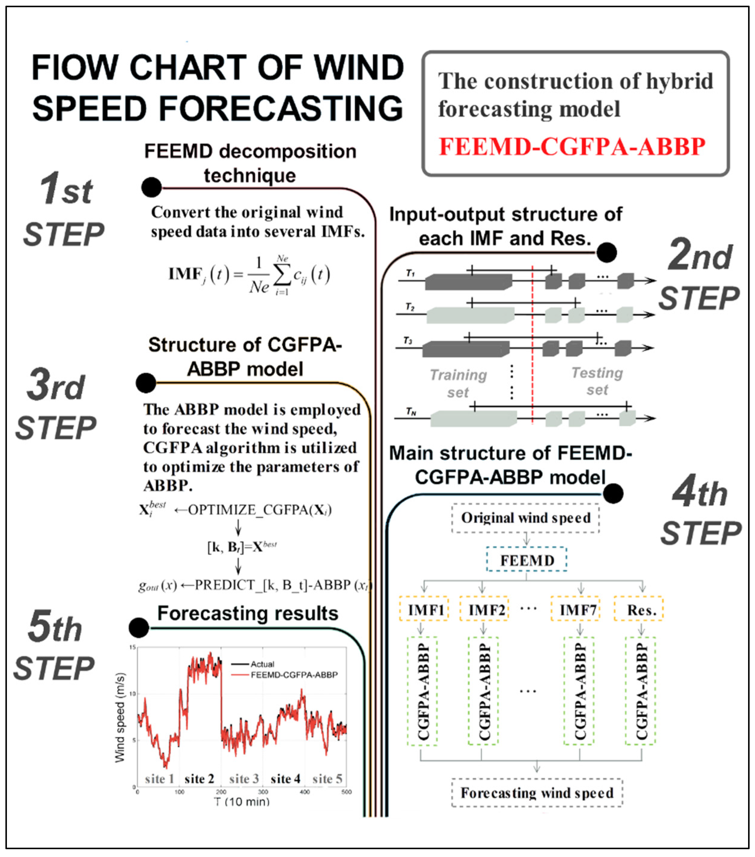
Due to the randomness and instability of wind series, a model based on the fast ensemble empirical mode decomposition technique is utilized to adaptively address the original wind speed series through decomposition into a finite number of intrinsic mode functions with a similarity property to modeling.
(2)
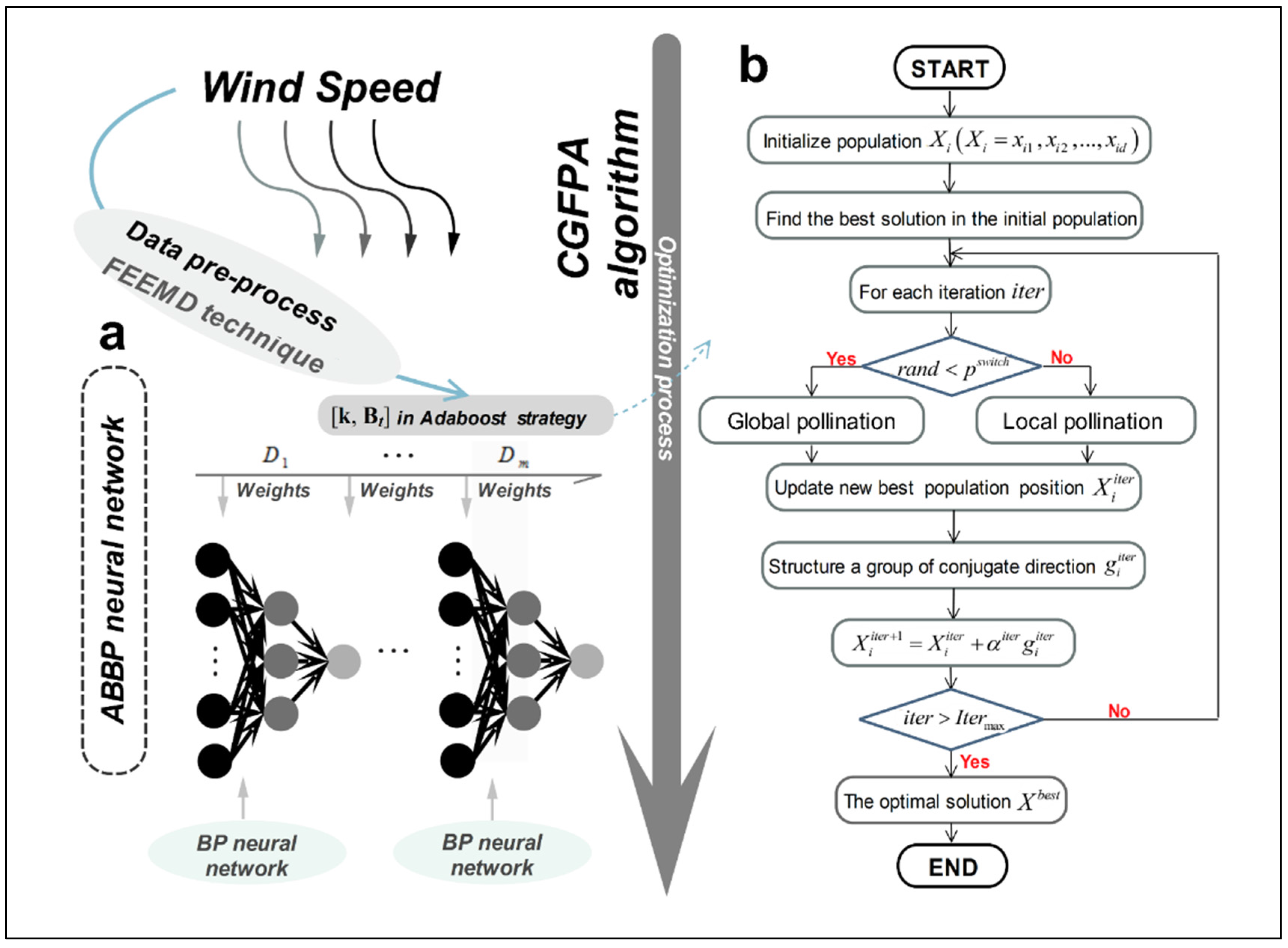
To overcome the drawbacks of the unstable forecasting results of the BP neural network, the ABBP model combined with the AB strategy is considered a strong predictor in this paper for wind-speed forecasting.
(3)
A novel modified algorithm, the CGFPA, is developed in the wind-speed forecasting field that, for the first time, chooses the parameter [ k ,   B t ] in the ABBP model for its better convergence and higher-quality solutions in lower iterations compared with the FPA.
(4)
Considering the skewness and kurtosis of the forecasting accuracy distribution, the forecasting availability, and the bias-variance framework, the Diebold-Mariano test is proposed to validate the accuracy and stability of the proposed model.
This paper is organized as follows. First, the concept of the models utilized in this paper, including the fast ensemble empirical mode decomposition technique, AB strategy, BP neural network and a modified optimization algorithm, the CGFPA, are outlined. Then, the modeling processes of the methods mentioned above are introduced. Simulation results are then presented and analyzed. The paper ends with an overall conclusion.

2. Methodology

In this section, the required individual tools will be presented concisely, including the fast ensemble empirical mode decomposition technique, the BP neural network, the AB technique, the FPA algorithm and the conjugate gradient method. The proposed hybrid approach will also be described in detail.

2.1. Fast Ensemble Empirical Mode Decomposition

The fast ensemble empirical mode decomposition technique is the development of the empirical mode decomposition and ensemble empirical mode decomposition techniques [46] (the details are shown in Appendix A). However, the empirical mode decomposition technique exhibits a potential mode-mixing problem that makes it unable to represent the characteristics of the original data. Wu and Huang developed the ensemble empirical mode decomposition to overcome this problem [46].

2.2. Artificial Neural Network (ANN)

In recent years, ANNs have been successfully utilized in a variety of applications as one of the most current artificial intelligence techniques [47,48]. In numerous neural network architectures, the most prevalent training method is the feed-forward neural network with back propagation (BP) training algorithm [27].
Theoretically, under the condition of appropriate weights and a reasonable structure, any nonlinear continuous functions can be approximated by the BP neural network. The principle of the BP neural network is to minimize the mean square error between the actual output value and that of the network by using the error gradient descent algorithm. The details of BPNN can be found in [27].

2.3. Adaptive Boosting (AB) Strategy

The AB strategy is one of the most excellent boosting algorithms in the big data mining field. It has a solid theoretical basis and has shown great success in practical applications [49]. Figure 1a shows the structure of ABBP neural network and the details are shown in Appendix B.

2.4. Optimization Algorithm-CGFPA

[k, Bt] is one of the most important factors directly influencing the calculation in the ABBP mode, and it thus influences the performance of the models. In this part, a brief introduction to the principles of the basic Flower Pollination Algorithm (FPA) and the Conjugate Gradient (CG) method is introduced, followed by the strategy of the combined optimization algorithm CGFPA.

2.4.1. Flower Pollination Algorithm (FPA)

A novel metaheuristic algorithm named the Flower Pollination Algorithm (FPA) was developed by Yang [50] in 2012 and was first used in wind-speed forecasts. The algorithm is inspired by the biological process of flower pollination.
The conjugate gradient (CG) method is an effective method between the Newton algorithm (NA) and the steepest descent algorithm (SDA) that overcomes the shortcomings of these two algorithms, including the slow convergence of the SDA and the shortcomings of the NA in which the Hesse matrix and inverse matrix must be stored and computed. The CG algorithm possesses advantages including a fast convergence rate and secondary termination. [51]. The details of CG and FPA as shown in Appendix C.

2.4.2. Modified Optimization Algorithm-CGFPA

The CG algorithm is carried out along a group of conjugate directions near the given point to search. It has abundant optimization information of the local area that can be employed. It also has a strong local search capability and is thus incorporated into the FPA algorithm to improve its local search capability and to improve the convergence speed and accuracy.
In every iteration of the CGFPA algorithm, the population position of a flower after updating is not directly fed into the next iteration process. Instead, it structures a group of conjugate directions g i i t e r + 1 through linear combination by employing the gradient g i i t e r at X i i t e r multiplied by the conjugate factor βiter and adding it to the negative gradient F ( x i i t e r + 1 ) of that point. Upon searching in this group of conjugate directions, the population position X i i t e r of the flower decreases sufficiently within a predetermined number of iterations. The (iter + 1)th iteration is re-entered after obtaining the position of the new population, and searching and updating continue, thus greatly enhancing the local optimization capability of the algorithm. In summary, the CGFPA algorithm organically combines the CG and the FPA algorithms to deliver strong global optimization and local searching capabilities. Figure 1b shows the flow chart of the CGFPA algorithm.
The pseudo-code of the CGFPA algorithm is summarized in Algorithm 1.
Algorithm 1: CGFPA (OPTIMIZE_CGFPA).
Parameters:
pswitch —the switch probability.
∇—the gradient operator (total differential in all direction of space).
N—the generation number of Xi.
iter—current iteration number.
Itermax —the maximum number of iteration.
1/*Initialize a population of N flowers Xi (Xi = xi1,xi2,…,xid) in random positions and initialize iter = 0.*/
2/*Find the best solution X i b e s t .*/
3while iter < Itermax do
4for i←1 to N do
5   if rand< pswitch then
6   Do global pollination x i i t e r . x i i t e r + 1 = x i i t e r + L * ( x i b e s t x i i t e r )
7   Else
8   Do local pollination x i i t e r + 1 . x i i t e r + 1 = x i i t e r + U * ( x j i t e r x k i t e r )
9   end if
10  /*Evaluate x i i t e r , replace x i i t e r by x i i t e r + 1 if the newly generation is better.*/
11   end for
12  /*Update the current best solution x i i t e r .*/
  Calculate g i i t e r = F ( x i i t e r ) .
  /*Calculate the gradient (search direction) g i i t e r .*/
  /*Determined searching step αiter by utilize the line search method.*/
  Let x i i t e r + 1 = x i i t e r + α i t e r g i i t e r + 1 and calculate g i i t e r + 1 = F ( x i i t e r + 1 ) .
13  iter = iter+1
14end do
15end while
16return Xbest.

3. Hybrid FEEMD-CGFPA-ABBP Model

In this part of the paper, we present the hybrid model FEEMD-CGFPA-ABBP for use in short-term wind-speed forecasting. First, the fast ensemble empirical mode decomposition technique will be utilized to decompose original wind-speed signals into several IMFs and one residual item that represents different frequency bands. The modified CGFPA algorithm will be employed to optimize the parameter [k, Bt] of the ABBP mode. Thus, the CGFPA-ABBP mode will be established to forecast each series after decomposition by the fast ensemble empirical mode decomposition technique, after overcoming the instability of the individual BP neural network. Figure 2 shows the structure of the proposed hybrid model. The sample data will be applied to train the ABBP mode. The pseudo-code of the hybrid model is provided in Algorithm 2.
Algorithm 2: FEEMD-CFFPA-ABBP (MODOL_HYBRID).
Input:
P—the input data matrix
Output:
T—the output data matrix
Parameters:
Ne—the ensemble number of trials.
α—the amplitude of added white noise.
M—the repeat times of trials
Θ—the critical point of updating the weight distribution.
k—the adjustment factor of the weight distribution.
Bt—the normalization factor.
(S, TFt, BTFt, BLFt)—the parameters of the BP neural network.
iterp—the number of weak predictors.
pswitch—the switch probability.
N—the generation number of Xi.
∇—the gradient operator (total differential in all spatial directions).
iter—current iteration number.
Itermax—the maximum number of iterations.
1IMFj(t)←PREPROCESSING_FEEMD(ri(t));
2/*Perform the following operations for each IMF.*/
3/*Initialize the weight distribution of m training sample Dt(i) = 1/m, error rate εn = 0.*/
4Sample normalization. xt = (xt xmin)/(xmax xmin).
5/*Weak predictor forecasting. By selecting different BP network functions, construct different types of weak predictors.*/
6for t←1 to iter do
7net = newff (P,T,S,TFt,BTFt,BLFt).
8/*Obtain the error rate εt of forecast series gt(x) and the distribution weights of the next weak predictor.*/
9for i←1 to m do
10  Find a best value of [k, Bt] by using optimization algorithm.
11   X i b e s t ←OPTIMIZE_CGFPA(Xi (Xi = xi1, xi2, …,xid))
12  iter = iter + 1.
13  /*[k,Bt] = Xbest.*/
14end do
15end do
16return gout (x).

3.1. Normalization and Preprocessing of Wind Speed Data

To enhance the wind speed accuracy of the ABBP mode, it is necessary to normalize the wind speed data. The original wind speed data are normalized according to Equation (1).
X s c a l e , i = X i X min , i X max , i X min , i
where, Xi represents the raw wind speed data; Xscale,i represents the normalization of the wind speed data; and Xmax,i and Xmin,i represent the maximum and minimum of the wind speed data, respectively.

3.2. Choice of Fitness Function

In evaluating the performance of the short-term wind-speed forecasting model, the root mean square error (RMSE) is used as the fitness function. The form of the function is shown in Equation (2),
f i t n e s s = 1 N i = 1 N ( x i x ^ i )
where N is the number of wind speed training samples; xi is the actual value of the wind speed; and x ^ i is the fitted value of the wind speed.

4. Experimentation Design and Results

To validate the effectiveness of the proposed novel hybrid model, this section describes three experiments based on comparisons with other models, with 10-min wind speed series at five different wind power stations.

4.1. Study Area and Datasets

Much attention has been given to research and development on renewable energy due to its high energy conversion and low pollution. As one form of renewable energy, wind-power generation can develop rapidly because of advantages such as huge volume, regeneration, wide distribution and no pollution. Wind energy is centralized in the northern, northwestern and eastern parts of China. This research considers the case of the wind power station in Penglai, Shandong Province. Figure 3 shows 10-min head wind speed data in January 2011 from five sites, including 1000 samplings in every site, collected randomly from Penglai. These five groups of data will be employed in the investigation of the forecasting performance. The 1st–900th samplings will be adopted as a training set to build forecasting models, and the 901st–1000th samplings will be used as a testing set to validate the models. The lateral data selection method is used to construct the training and testing sets [40]. The standard deviations are 2.38 (m/s), 3.02 (m/s), 2.58 (m/s), 2.37 (m/s) and 2.87 (m/s), respectively, which implies that the wind-speed series fluctuates significantly with the minimum/maximum of Sites 1–5, which are 2.05/16.10 (m/s), 1.96/17.56 (m/s), 2.26/4.86 (m/s), 2.65/12.34 (m/s) and 3.61/16.55 (m/s), respectively. This result can be intuitively observed from the amplitude and frequency of the series fluctuations, which can change from very high to low values, and vice versa.

4.2. Evaluation Criteria of Forecast Performance

Forecasting accuracy is an important criterion in the evaluation of forecasting models. In this paper, we use four different evaluation criteria, including AE (average error), MAE (mean absolute error), MSE (mean square error), MAPE (mean absolute percentage error) and ω (promotion rate of forecasting capability). The forecast validation method chooses the model via the smallest AE, MAE, MSE and MAPE, and ω is utilized to quantitatively compare the enhancement ability of the strong predictor.
A E = 1 N i = 1 N ( x i x ^ i )
M A E = 1 N i = 1 N | x i x ^ i |
M S E = 1 N i = 1 N ( x i x ^ i ) 2
M A P E = 1 N i = 1 N | x i x ^ i x i | × 100 %
where x and x ^ represent the actual value and forecasting value, respectively, and N is the total number of data used for the performance evaluation and comparison.
ω ( t ) = | e r r o r 1 e r r o r 2 ( t ) e r r o r 1 | × 100 %
where
e r r o r 1 = 1 N i = 1 N | x ( i ) x ^ s ( i ) x ( i ) | × 100 %
e r r o r 2 ( t ) = 1 N i = 1 N | x ( i ) x ^ t ( i ) x ( i ) | × 100 %
where, x ^ s is the forecast value utilizing a strong predictor, and x ^ t is the forecast value using the tth weak predictor.

4.3. Experimental Setup

In this section, the experiments are divided into three parts: Experiment I, Experiment II and Experiment III. In Experiment I, the performance of the FEEMD-ABBP model is compared with the ABBP mode to confirm the significance of the fast ensemble empirical mode decomposition technique in wind-speed forecasting. In Experiment II, the performance of the hybrid ABBP mode is compared with 10 individual BP neural networks to improve the forecasting accuracy and generalization capability of the individual neural network. In Experiment III, the proposed hybrid model FEEMD-CGFPA-ABBP is compared with other forecasting models, namely, FEEMD-ABBP, ABBP, the conventional BP neural network and the ARIMA model. To confirm the universality of the proposed model, Experiment I, Experiment II and Experiment III are validated at five different sites.
All algorithms are operated on the following platform: 3.20 GHz CPU, 8.00 GB RAM, Windows 7, and MATLAB R2012a. The experimental parameters are shown in Table 1. Meanwhile, taking into account randomness factors and ensuring that the final results are reliable and independent of the initial weights, we carry out each experiment 50 times and then take the average value.

4.3.1. Experiment I: Results of Data Preprocessing

Many methods such as empirical mode decomposition, ensemble empirical mode decomposition and fast ensemble empirical mode decomposition are available to enhance the forecasting performance of wind speed series. In this paper, we utilize the fast ensemble empirical mode decomposition technique, which combines the fast ensemble empirical mode decomposition with a series of selected computational parameters to guarantee good time performance when addressing the original wind speed series in the data preprocessing stage. In the fast ensemble empirical mode decomposition stage, the wind speed series is decomposed into seven IMFs and one residue. Figure 4 shows the original wind speed series and its subsequences with their frequency by the fast ensemble empirical mode decomposition technique for the five sites. Table 2 shows the results of the FEEMD-ABBP and ABBP models in terms of four criteria, AE, MAE, MSE, and MAPE. Figure 5 shows the detailed forecasting results of the FEEMD-ABBP and ABBP models. Figure 4, Table 2 and Figure 5 indicate the following:
(1)
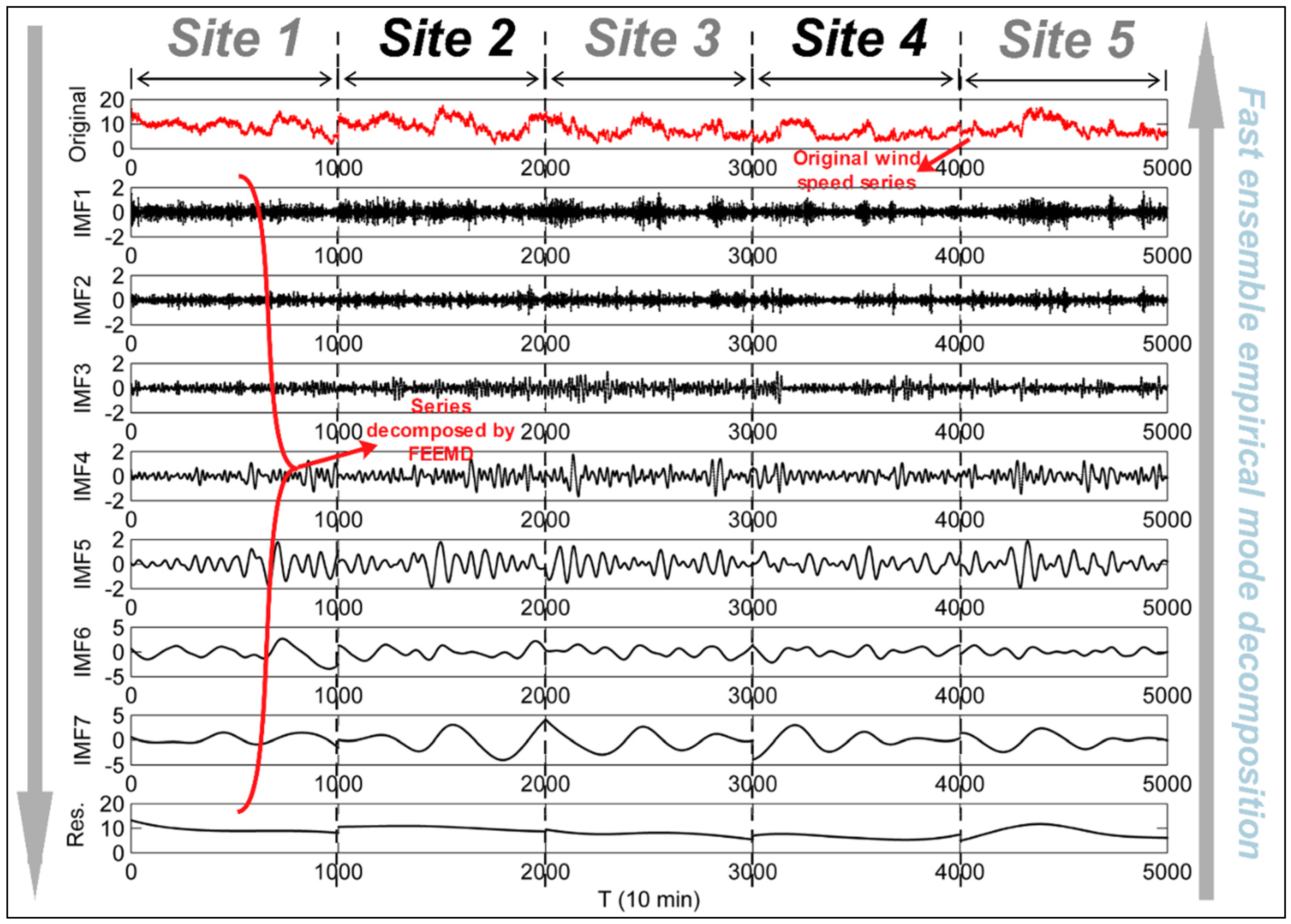
The extracted IMFs are graphically indicated to illustrate the order of frequency from highest the lowest. The high- and low-frequency entries are given in the first few and last few IMFs, respectively. The former represent high noise or time variation in the original wind speed series, while the latter represent long-period IMFs. In addition, the shifting residue, the last component, generally represents the trend of the wind speed series. It can be clearly determined that the sub-series (IMF7) with the lowest frequency indicates that the major fluctuation of the raw wind speed series is highly similar to the original wind speed series.
(2)
When processing the original series using the fast ensemble empirical mode decomposition technique, different characteristic information can be extracted at different scales, leading to the strong regularity and simple frequency components of each IMF. The local fluctuations of the original series can also be fully captured using this method. Moreover, because of the similar frequency characteristics of each IMF, it is beneficial to reduce the complexity and enhance the efficiency and accuracy of the ABBP forecasting model.
(3)
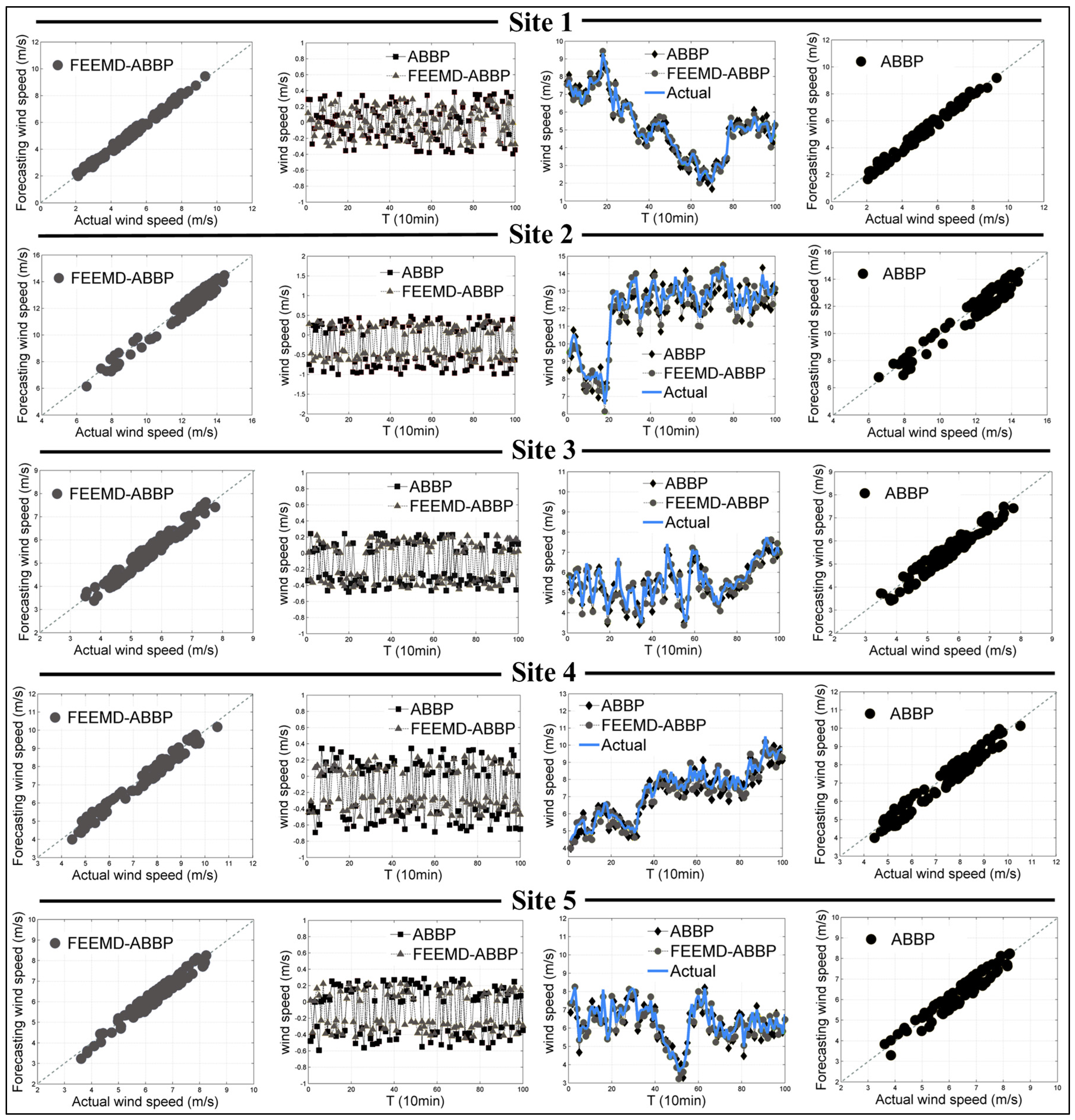
The bold entries in Table 2 indicate the values of AE, MAE, MSE and MAPE that are the smallest among the FEEMD-ABBP and ABBP models. In this model comparison, it can be clearly observed that the fast ensemble empirical mode decomposition technology employed on the ABBP model performs better than the single ABBP model at all five sites. The MAPEs achieved by the FEEMD-ABBP model at the five sites are 3.2354%, 3.3234%, 4.2093%, 3.7402% and 3.754%, representing decreases of 1.2912%, 1.2432%, 0.6224%, 1.1648% and 0.6972%, respectively.

4.3.2. Experiment II: Strong Predictor (ABBP Model) vs. Weak Predictors

Because the traditional BP neural network usually encounters defects such as easily falling into local minima and low forecasting precision, we employed the AB strategy integrated into the BP neural networks as a strong predictor to enhance the forecasting accuracy generalization ability of the neural network. First, the AB strategy preprocesses the historical data and initializes the distribution weights of the test data. Second, it selects different hidden layer nodes, node transfer functions, training functions and network learning functions to construct weak predictors of the BP neural networks and then repeatedly trains the sample data. In the end, the AB strategy was employed to combine the different BP neural networks to form a new strong predictor.
The function of the BP neural network constructed in MATLAB is net = newff(P, T, S, TFt, BTFt, BLFt). Here, P represents the input wind speed data matrix, T represents the output wind speed data matrix, S represents the nodes of the hidden layer, T F t represents the node transfer function, B T F t represents the training function, and B T F t represents the network learning function. Upon adjusting the parameters, including S, TFt, BTFt, and BLFt, different types of BP weak predictors were constructed. In Experiment II, ten BP neural networks were employed to form the weak predictor series.
Table 3 indicates the promotion rate of the forecasting capability by using the strong predictor compared with the ten weak predictors. From Table 3, compared with the forecasts of the ten weak predictors at the five data sites, there are significant improvements for the strong predictor forecasts. For example, at Site 1, the ω of the strong predictor compared with that of weak predictors 1 through 10 is increased by 36.3386%, 35.2563%, 40.2408%, 31.1205%, 20.4267%, 18.3870%, 33.0996%, 33.5240%, 32.4778% and 25.7482%, respectively. The values in bold represent the largest ω among the ten weak predictors. The largest ω in the Sites 1 through 5 were 40.2408%, 34.9932, 70.6485%, 60.5825% and 86.1126%, respectively. Over all, the strong predictor ABBP mode has the best performance at all five data sites. There is no weak predictor that offers a low MAPE value at any of the five sites. Meanwhile, the ABBP mode is more stable than the other weak predictors. Experiment II indicates the rationality and effectiveness of the ABBP mode based on the AB strategy for application in wind-speed forecasting.

4.3.3. Experiment III: Forecasting Comparison Results

In this part, the proposed hybrid model FEEMD-CGFPA-ABBP is compared with other forecasting models, namely, the FEEMD-ABBP, ABBP, conventional BP neural network and ARIMA models. In addition, to further evaluate the proposed hybrid model, FEEMD-ELM and FEEMD-SVR is utilized to compare. The results indicate in Table 4 and Table 5 and Figure 6:
(1)
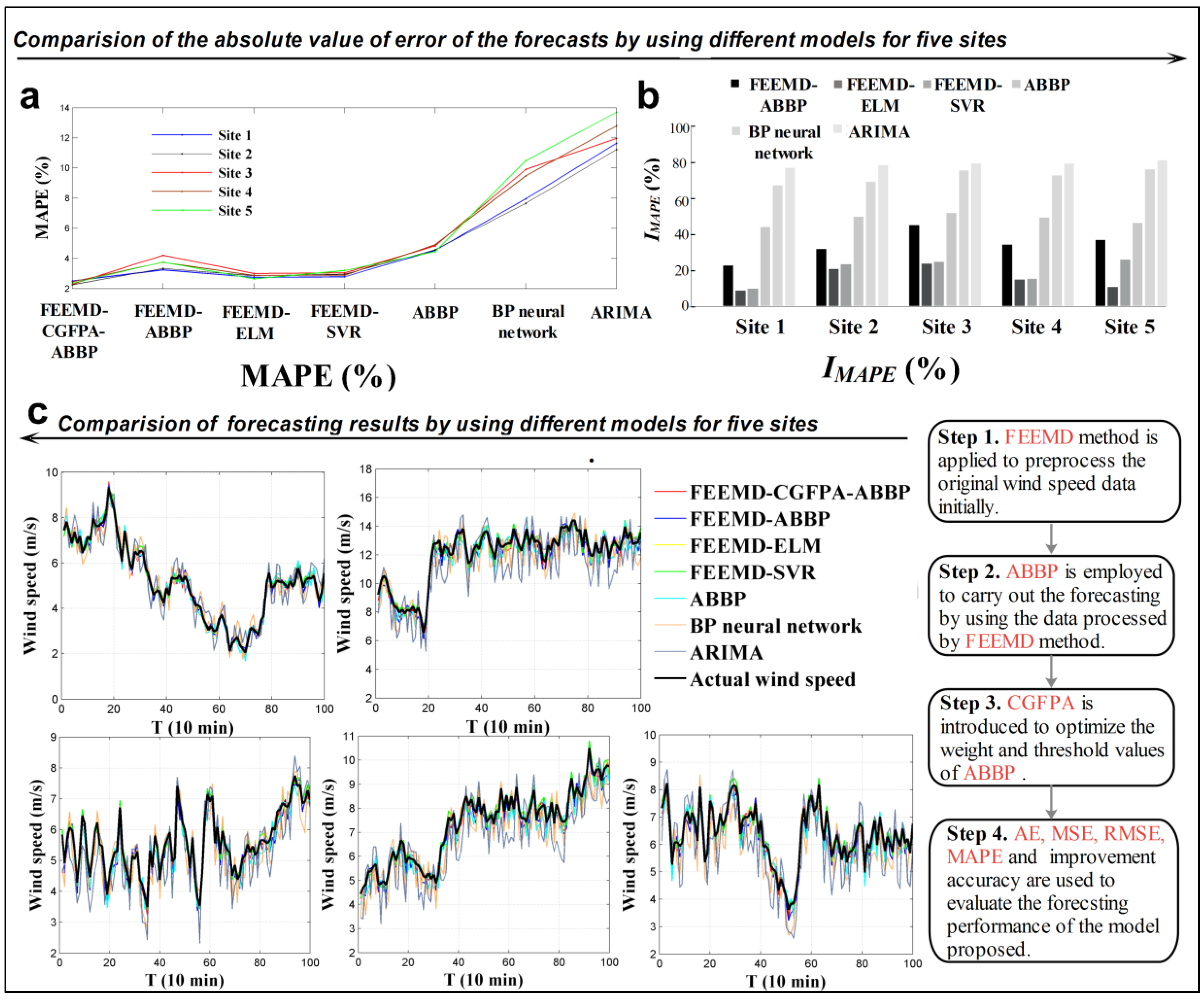
The AE, MAE, MSE and MAPE values are calculated for the forecasts, and the corresponding results are compiled and presented in Table 4. The values in bold represent the AE, MAE, MSE, and MAPE values that are the lowest among all the forecasting models at the five sites. It can be clearly seen that the proposed hybrid model has the highest accuracy at all wind farm sites, with MAPE values of 2.4976%, 2.2495%, 2.2785%, 2.4397% and 2.3483% at Sites 1 through 5, respectively.
(2)
To compare the different performances between two forecasting models, the improvement accuracy is used, which is defined as
I E C = E C 1 - E C 2 E C 1 × 100 %
where EC is the value of one of the forecasting performance evaluation criteria AE, MAE, MSE or MAPE. EC1 and EC2 denote the values of the evaluation criterion generated by the compared models (FEEMD-ABBP, FEEMD-ELM, FEEMD-SVR, ABBP, BP neural network, and ARIMA) and the proposed hybrid model. Table 5 shows the corresponding improvement of the proposed model. From Table 5, compared with the other forecasting models among all five sites, there are significant improvements for the proposed model forecast. For example, at Site 2, the FEEMD-CGFPA-ABBP model leads to 11.9941%, 18.6508%, 2257.8947%, 3589.362%, 62.2130% and 77.009% reductions in AE, 31.0846%, 35.0349%, 23.6241%, 28.5597%, 71.2193% and 80.0101% reductions in MAE, 51.0923%, 69.649%, 26.8657%, 36.8195%, 91.9141% and 96.1417% reductions in MSE, and 32.3128%, 41.4833%, 20.9092%, 23.4968%, 70.5879% and 79.9484% reductions in MAPE in comparison to FEEMD-ABBP, FEEMD-ELM, FEEMD-SVR, ABBP, BP neural network and ARIMA, respectively. Additionally, the maximum decreases in MAE, MSE and MAPE for the proposed hybrid model among all five sites are 82.3511%, 96.7654% and 86.8612%, respectively.
(3)
Figure 6 illustrates the evaluation criterion values of the forecasts offered by the proposed hybrid model and that offered by the other models among the five sites. It is clearly indicated that the FEEMD-CGFPA-ABBP model can provide high and stable forecasting accuracy.
By comparison with the forecasting models employed here, it can be concluded that the proposed FEEMD-CGFPA-ABBP model can obtain more information reflecting the real wind-speed fluctuations, leading to a better wind-speed forecasting performance at the five wind farm sites in Penglai, Shandong Province. Therefore, the proposed hybrid model provides an option for 10 min wind-speed forecasting and should be taken into consideration when searching for the best 10 min wind-speed forecasting model.

5. Discussion

In this section, tests related to the proposed hybrid model that would affect the forecasting performance are discussed. We first present an evaluation metric, namely, the forecasting availability, to analyze and evaluate the quality of the wind-speed forecasting. The bias-variance framework is then utilized to evaluate the effectiveness of the forecast models. Furthermore, hypothesis testing is employed to examine the forecasting performance.

5.1. Forecasting Availability

The forecasting availability can be measured not only by the square sum of the forecasting error but also by the mean and mean squared deviation of the forecasting accuracy. In certain practical circumstances, the skewness and kurtosis of the forecasting accuracy distribution needs further consideration, so the forecast availability is presented to solve this problem.
The 1st-order forecasting availability is the expected forecasting accuracy sequence, and the 2nd-order forecasting availability is the difference between the expectation and the standard deviation of the forecasting accuracy sequence. We use the forecasting availability to evaluate the wind-speed forecasts [52]. Table 6 shows that the 1st-order and 2nd-order forecasting availabilities offered by the proposed hybrid model FEEMD-CGFPA-ABBP outperform those of the other models at the five sites. For example, at Site 1, the 1st-order forecasting availabilities offered by the hybrid model, FEEMD-ABBP, FEEMD-ELM, FEEMD-SVR, ABBP, BP neural network and ARIMA are 0.9750, 0.9676, 0.9701, 0.9687, 0.9547, 0.9205 and 0.8837, respectively, while their 2nd-order values are 0.9618, 0.9457, 0.9534, 0.9523, 0.9214, 0.8651 and 0.8143. Thus, the hybrid model is a more valid model than the others.

5.2. Bias-Variance Framework

The bias-variance framework [53] is utilized to estimate the models’ accuracy and stability, which are important in evaluating the effectiveness of the wind-speed forecasting models. The error attributed to bias is taken as the difference between the forecasts of the proposed model and the observed value. The error attribute to variance is taken as the variability of the forecasting results.
Let x i x ^ i be the difference between the actual value xi and the forecasting value x ^ i . The expectation of the forecasting value over all the forecasting data is E ( x ^ ) = 1 N i = 1 N x ^ i , and the expectation of the observed value is x = 1 N i = 1 N x i , where N is the number of data for comparison. The bias-variance framework is decomposed as follows:
E ( x ^ x ) 2 = E [ x ^ E ( x ^ ) + E ( x ^ ) x ] 2 = E [ x ^ E ( x ^ ) ] 2 + [ E ( x ^ ) x ] 2 = V a r ( x ^ ) + B i a s 2 ( x ^ )
B i a s ( x ^ ) demonstrates superior forecast accuracy in the model. Similarly, a smaller V a r ( x ^ ) indicates superior stability.
Table 7 shows that the absolute values of the biases of the other models are larger than those of the FEEMD-CGFPA-ABBP model, which reveals that the proposed model is more accurate. The variance results demonstrate that the hybrid model is more stable. Thus, it is clear that the proposed hybrid model has a higher accuracy and stability in wind-speed forecasting and that it performs much better than the individual models in forecasting.

5.3. Test of Hypothesis

The test of hypothesis is a statistical inference method different from the exploratory data analysis, which may have no hypotheses defined beforehand. The test is applied to determine under what circumstance a trial would result in a null hypothesis rejection under a level of significance defined beforehand. Commonly, a dataset obtained by an idealized model is compared against a dataset achieved by sampling. The comparison is considered statistically significant in case the relationship between the datasets would be the null hypothesis, which is unlikely to occur based on the significance level. By using hypothesis testing, we can quantify our level of confidence that the difference is real.
In this part, we examine the efficiency of the proposed hybrid model by applying one of the hypothesis tests, namely, the Diebold-Mariano test [54]. The hypothesis test is defined as
H 0 : E [ L ( ε t 1 ) ] = E [ L ( ε t 2 ) ]
H 1 : E [ L ( ε t 1 ) ] E [ L ( ε t 2 ) ]
where L(∙) is the loss function, two popular versions of which are MAE and MSE, and ε t 1 and ε t 2   are the forecasting errors of the two competing forecasts.
The Diebold-Mariano statistic is convergent in distribution in a normal distribution, which, based on parameter Dt, is expressed as D t = L ( ε t 1 ) L ( ε t 2 ) . Comparing the absolute value of the Diebold-Mariano statistic with that of the critical value zα/2 of the standard normal distribution N(0,1), the null hypothesis will be rejected if the Diebold-Mariano statistic falls outside the interval [−zα/2, zα/2], where α represents the significance level, considering the difference between the forecasting ability of two types of model to be significant. Table 7 shows the Diebold-Mariano value based on the MAE loss function. The result indicates that the Diebold-Mariano values of the FEEMD-ABBP, the FEEMD-ELM and the FEEMD-SVR models are larger than the upper limits at the 5% significance level, and the Diebold-Mariano values of the ABBP, BP and ARIMA models are all larger than the upper limits at the 1% significance level. This result also indicates that the proposed hybrid model is significantly superior to other models, as the upper limits at the different significance levels are smaller than the Diebold-Mariano statistics in all cases. Thus, it is obvious that the proposed hybrid FEEMD-CGFPA-ABBP model significantly outperforms the other four models. Consequently, although the proposed hybrid model is not simple, it is able to satisfactorily approximate the actual wind speed, and it can be an effective tool in mining and analysis for wind power plants.

6. Conclusions

Today, power systems face growing challenges in maintaining a secure and reliable energy supply. Wind energy is gradually become one of the fastest growing clean and renewable energy sources for power generation. To integrate wind energy into the power system, it is important to forecast wind power generation. Wind speed is affected by various environmental factors, so wind speed data present high fluctuations, autocorrelation and stochastic volatility, and it is difficult to forecast wind speed using a single model. In this paper, we proposed a novel hybrid FEEMD-CGFPA-ABBP model based on AB strategy and CGFPA algorithm. Through the analysis, the conclusions are as follow:
(1)
The BP neural network can handle data with nonlinear features, and the AB strategy integrated with BP neural networks is adopted to overcome the uncertainty of the outcomes that can be attributed to the randomness of the initialization of the BP neural networks.
(2)
The modified CGFPA algorithm is utilized to optimize the parameters in the ABBP mode.
(3)
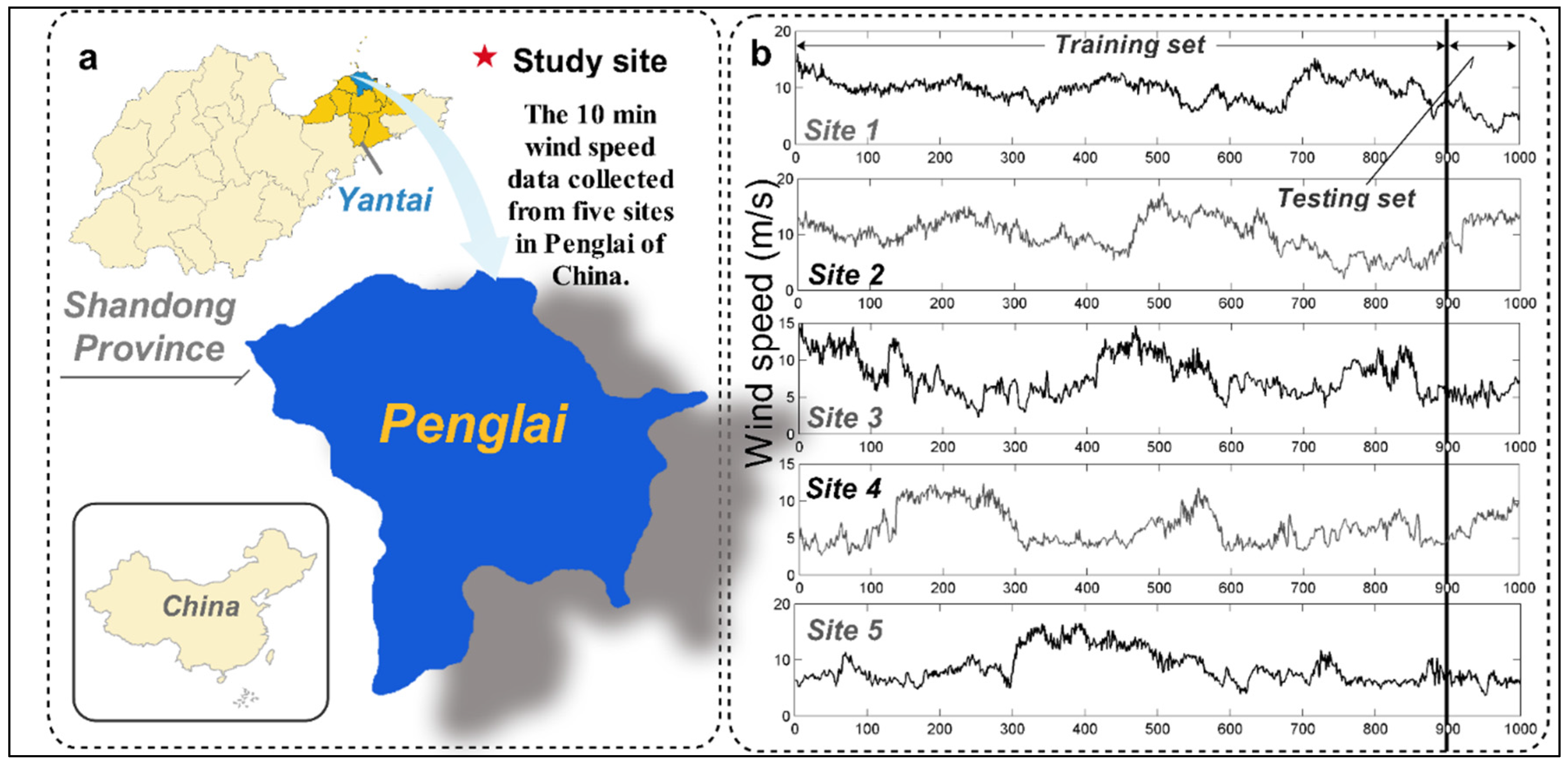
The experimental study of the wind-speed forecasting in five sites in Penglai, Shandong Province, China, effectively proves that the proposed hybrid model has higher precision and stability than FEEMD-ABBP, ABBP and other forecasting models.
Thus, the proposed FEEMD-CGFPA-ABBP model, which has high precision, is a promising model for use in the future. This hybrid model can also be applied in many other fields, such as tourism demand, product sales, power load, and traffic-flow forecasting.

Acknowledgments

This work was financially supported by the National Natural Science Foundation of China (71171102).

Author Contributions

J.H. and C.W. conceived and designed the experiments; J.H. performed the experiments; J.H. and X.Z. analyzed the data; L.X. contributed reagents/materials/analysis tools; J.H. wrote the paper.

Conflicts of Interest

The authors declare no conflict of interest.

Appendix A

Appendix A1. Empirical Mode Decomposition

Definition 1. Time series x(t) can be decomposed and expressed using the formula
x ( t ) = i = 1 n I M F i ( t ) + r n ( t )
where IMFi (t), (i = 1,2,…,n) represents the intrinsic mode functions (i.e., local oscillation) decomposed by empirical mode decomposition, and rn (t) is the nth residue (i.e., local trend).
Definition 2. The stoppage criterion is defined as
S D j = t = 0 T | h i , j 1 ( t ) h i , j ( t ) | 2 [ h i , j 1 ( t ) ] 2
The sifting process stops when a pre-given value is larger than SDj. The process of decomposition is over when the value of SDj is between 0.2 and 0.3.
The pseudo-code of the empirical mode decomposition technique is provided in Algorithm A1.
Algorithm A1: Empirical Mode Decomposition (PREPROCESSING_EMD).
Parameters:
δ—a random number between 0.2 and 0.3.
T—the series length.
1/*Initialize residue r0(t) = x(t), i = 1, j = 0; Extract local maxima and minima of ri-1(t).*/
2for j = j + 1 do
3for i←1 to n do
4  while (SDj < δ) do
5   Calculate the upper envelope Ui (t) and Li (t) by cubic spline interpolation.
6   Mean envelope m ¯ i (t) = [Ui (t) + Li (t)]/2; the ith component ri (t) = ri-1(t) − m ¯ i (t).
7   /*ri,j(t) = hi(t); m ¯ i,j(t) be the mean envelope of ri,j(t).*/
8   end while
9  Calculate ri, j (t) = ri, j-1(t) − m ¯ i, j-1(t)
10  /*Let jth IMF as IMFi(t) = r i , j(t).*/
11  /*Update the residue ri(t) = ri-1(t) − IMFi(t).*/
12end do
13end do
14return x(t)

Appendix A2. Ensemble Empirical Mode Decomposition

Definition 1. The corresponding IMF ensemble empirical mode decomposition based on empirical mode decomposition is expressed as
I M F j ( t ) = 1 N e i = 1 N e c i j ( t )
where Ne is the ensemble number and cij(t) is the jth IMF of the ith added noise series.
Definition 2. The influence of the added white noise can be determined by the rule
ε n = ε N e
where εn is the standard deviation of the error, defined as the difference between the corresponding IMFs and the input signals, and ε is the amplitude of the added white noise.
The pseudo-code of the ensemble empirical mode decomposition technique is provided in Algorithm A2.
Algorithm A2: Ensemble Empirical Mode Decomposition.
Parameters:
Ne—the ensemble number of trials.
α—the amplitude of added white noise.
1/*Obtain series ri(t) by adding white noise series N = {n1, n2,…, nNe} to series y(t).*/
2for j = j + 1 do
3for i←1 to n do
4  ri (t) = y(t) + αni (t).
5  cij(t)←PREPROCESSING_EMD(ri ( t ) );
6  /* Repeat M trials.*/
7end do
8end do
9Calculate the corresponding IMFs of the decomposition IMFj(t)
10return IMFj(t)

Appendix A3. Fast Ensemble Empirical Mode Decomposition

The pseudo-code of the fast ensemble empirical mode decomposition technique is provided in Algorithm A3.
Algorithm A3: Fast Ensemble Empirical Mode Decomposition (PREPROCESSING_FEEMD).
Parameters:
Ne—the ensemble number of trials.
α—the amplitude of added white noise.
M—the number of repeats of each trial
1foreach times←1 to M do
2/*Obtain series ri(t) by adding white noise series N = {n1, n2,…, nNe} to series y(t).*/
3for j = j + 1 do
4  for i←1 to n do
5   ri (t) = y(t) + αni (t).
6   cij(t)←PREPROCESSING_EMD(ri ( t ) );
7   /*sampling data at some points of series ri(t).*/
8   end do
9end do
10end for
11Calculate the corresponding IMFs of the decomposition IMFj(t)
12return y(t) = j n I M F j ( t )

Appendix B

Appendix B1. Adaptive Boosting (AB) Strategy

Definition 1. The main goals of the AB strategy are to (1) Establish weak predictors with the same weight given to each test sample; (2) Adjust the test sample weights according to the results of the forecasting precision. The sample weights of low forecasting accuracy are strengthened, and those of high forecasting accuracy are abated; (3) After constant adjustment, we end up with a group of weak predictor sequences and their weights; the weak predictor series are combined into a strong predictor.
Definition 2. The error rate of each weak predictor’s forecast gt (x) is expressed as
ε t = i = 1 m D t ( i )
where εt and Dt (i) represent the error rate and the weight distribution, respectively, and m is the training sample number.
Definition 3. The test sample weight after adjustment is
D t ( i ) = { k D t ( i ) σ > Θ D t ( i ) σ Θ
D t + 1 ( i ) = D t ( i ) B t
where k represents the adjustment factor of the weight distribution, Bt represents the normalization factor, and σ is the training error. Θ is set as 10−4.
Definition 4. The strong predictor is
g o u t ( x ) = t = 1 i t e r { ( log 1 ε t 2 ) g t ( x ) } / t = 1 i t e r ( log 1 ε t 2 )
where iter is the number of weak predictors.

Appendix B2. ABBP Mode

The algorithm of the ABBP mode is outlined as Algorithm B1.
Algorithm B1: ABBP (PREDICT_ABBP).
Input:
P—the input data matrix
Output:
T—the output data matrix
Parameters:
Θ—the critical point of updating the weight distribution.
k—the adjustment factor of weight distribution.
Bt—the normalization factor.
(S, TFt, BTFt, BLFt)—the parameters of BP neural network in MATLAB.
iter —the number of weak predictors
1/*Initialize the weight distribution of m training sample Dt(i) = 1/m, error rate εn = 0.*/
2Sample normalization. xt = (xt xmin)/(xmax xmin).
3/*Weak predictor forecasting. By selecting different BP network functions, construct different types of weak predictors.*/
4for t←1 to iter do
5net = newff (P,T,S,TFt,BTFt,BLFt).
6/*Obtain the error rate εt of forecast series gt(x) and the distribution weights of the next weak predictor.*/
7for i←1 to m do
8  /*Adjustment of test sample data weights.*/
  Dt+1(i) = Dt (i) / Bt.
   D t ( i ) = { k D t ( i ) , σ > Θ D t ( i ) , σ Θ  
9  /*Output strong predictor function.*/
10end do
11end do
12return gout (x)

Appendix C

Appendix C1. Flower Pollination Algorithm (FPA)

Definition 1. (1) Global pollination process: Biotic pollination is a cross-pollination process that can be regarded as global, as the movement of pollinators carrying pollen occurs via Lévy flights; (2) Pollination behavior: The process of abiotic or self-pollination is the source of local pollination; (3) Flower constancy: The constancy of the flower is equal to the probability of reproduction, which is proportional to the similarity of the flowers involved. (4) p ∈ [0,1] is the switch probability, which is utilized to control the local and global pollination.
Definition 2. Formulate the algorithm as follows:
(1) The global pollination process and flower constancy are represented as
x i i t e r + 1 = x i i t e r + L ( x i b e s t x i i t e r )
where x i i t e r is pollen i at iteration iter and x i b e s t is the best solution. L* represents Lévy flights, which are used to represent the movements of the pollinators. The Lévy distribution represents the strength of the pollination. λ is the distribution factor and ranges from 0.3 to 1.99 [37]. The Lévy distribution is represented as
L λ Γ ( λ ) sin ( π λ / 2 ) π s ( 1 + λ ) ( s s 0 > 0 )
In Equation (A10), Γ (λ) is the standard gamma function. s is indicated in Equation (A11), where rnd1 and rnd2 are two random numbers obeying a Gaussian distribution.
s = r n d 1 | r n d 2 | 1 / λ ;   r n d 1 N ( 0 , σ 2 ) , r n d 2 N ( 0 , 1 )
σ 2 = { Γ ( 1 + λ ) λ Γ [ ( 1 + λ ) / 2 ] sin ( π λ / 2 ) 2 ( λ 1 ) / 2 } 1 / λ
(2) The local pollination process and flower constancy are represented as:
x i i t e r + 1 = x i i t e r + U ( x j i t e r x k i t e r )
where, x j i t e r and x k i t e r are pollen from different flowers of a plant of the same family. U* obeys a uniform distribution over [0, 1].
(3) According to Ref. [38], we set the best value of the switch probability pswitch to be equal to 0.8.

Appendix C2. Conjugate Gradient

Definition 1. The basic idea of the CG algorithm is to combine the conjugate with the SDA, constructing a group of conjugate directions by utilizing the gradient at a given point. That is, when the dimension of a function is g, it is necessary to produce g search directions that are linearly independent and mutually conjugated. The search direction is expressed as
g i i t e r + 1 = { g i i t e r i t e r = 0 g i i t e r + β i t e r g i i t e r 1 i t e r 0
where the factor of the conjugate is
β i t e r = F ( x i i t e r ) 2 F ( x i i t e r 1 ) 2
where, F(x) is the objective function, g i 0 = F ( x i 0 ) .
This method has the characteristics of a second termination (i.e., it will reach the minimum point after limited iterations when used in a secondary convex function).

References

  1. Hui, L.; Tian, H.Q.; Li, Y.F.; Lei, Z. Comparison of four adaboost algorithm based artificial neural networks in wind speed predictions. Energy Convers. Manag. 2015, 92, 67–81. [Google Scholar]
  2. New Record in Worldwide Wind Installations. Available online: http://www.wwindea.org/new-record-in-worldwide-wind-installations/ (accessed on 5 February 2015).
  3. Ferreira, C.; Gama, J.; Matias, L.; Botterud, A.; Wang, J. A survey on wind power ramp forecasting. In Report ANL/DIS; Argonne National Laboratory: Northeast Illinois, United State, 2011; volume 5, pp. 10–13. [Google Scholar]
  4. Ferreira, C.A.; Gama, J.; Costa, V.S.; Miranda, V.; Botterud, A. Predicting Ramp Events with a Stream-Based HMM Framework. Discovery Science; Springer Berlin Heidelberg: Berlin, Germany, 2012; pp. 224–238. [Google Scholar]
  5. Wang, J.Z.; Wang, Y.; Jiang, P. The study and application of a novel hybrid forecasting model—A case study of wind speed forecasting in china. Appl. Energy 2015, 143, 472–488. [Google Scholar] [CrossRef]
  6. Goh, S.L.; Chen, M.; Popovi, D.H.; Aihara, K.; Obradovic, D.; Mandic, D.P. Complex-valued forecasting of wind profile. Renew. Energy 2006, 31, 1733–1750. [Google Scholar] [CrossRef]
  7. Wang, J.; Zhang, W.; Wang, J.; Han, T.; Kong, L. A novel hybrid approach for wind speed prediction. Inform. Sci. 2014, 273, 304–318. [Google Scholar] [CrossRef]
  8. Lei, M.; Shiyan, L.; Chuanwen, J.; Hongling, L.; Yan, Z. A review on the forecasting of wind speed and generated power. Renew. Sustain. Energy Rev. 2009, 13, 915–920. [Google Scholar] [CrossRef]
  9. Salcedo-Sanz, S.; Pérez-Bellido, A.M.; Ortiz-García, E.G.; Portilla-Figueras, A.; Prieto, L.; Paredes, D. Hybridizing the fifth generation mesoscale model with artificial neural networks for short-term wind speed prediction. Renew. Energy 2009, 23, 1451–1457. [Google Scholar] [CrossRef]
  10. Salcedo-Sanz, S.; Pérez-Bellido, A.M.; Ortiz-García, E.G.; Portilla-Figueras, A.; Prieto, L.; Correoso, F. Accurate short-term wind speed prediction by exploiting diversity in input data using banks of artificial neural networks. Neurocomputing 2009, 72, 1336–1341. [Google Scholar] [CrossRef]
  11. Khashei, M.; Bijari, M.; Raissi-Ardali, G. Improvement of Auto-Regressive Integrated Moving Average Models Using Fuzzy Logic and Artificial Neural Networks (ANNs). Neurocomputing 2009, 72, 956–967. [Google Scholar] [CrossRef]
  12. Salcedo-Sanz, S.; Ortiz-García, E.G.; Pérez-Bellido, A.M.; Portilla-Figueras, J.A.; Prieto, L.; Paredes, D.; Correoso, F. Performance comparison of multilayer perceptrons and support vector machines in a short-term wind speed prediction problem. Neural Netw. World 2009, 19, 37–51. [Google Scholar]
  13. Pourmousavi Kani, S.A.; Ardehali, M.M. Very short-term wind speed prediction: A new artificial neural network-Markov chain model. Energy Convers. Manag. 2011, 52, 738–745. [Google Scholar] [CrossRef]
  14. Zhang, W.; Wang, J.; Wang, J.; Zhao, Z.; Tian, M. Short-term wind speed forecasting based on a hybrid model. Appl. Soft Comput. 2013, 13, 3225–3233. [Google Scholar] [CrossRef]
  15. Landberg, L. Short-term prediction of the power production from wind farms. J. Wind Eng. Ind. Aerodyn. 1999, 80, 207–220. [Google Scholar] [CrossRef]
  16. Alexiadis, M.C.; Dokopoulos, P.S.; Sahsamanoglou, H.S.; Manousaridis, I.M. Short term forecasting of wind speed and related electrical power. Sol. Energy 1998, 63, 61–68. [Google Scholar] [CrossRef]
  17. Negnevitsky, M.; Potter, C.W. Innovative short-term wind generation prediction techniques. In Proceedings of the Power Systems Conference and Exposition, Atlanta, GA, USA, 29 October–1 November 2006; pp. 60–65.
  18. Kulkarni, M.; Patil, S.; Rama, G.; Sen, P. Wind speed prediction using statistical regression and neural network. J. Earth Syst. Sci. 2008, 117, 457–463. [Google Scholar] [CrossRef]
  19. Kavasseri, R.G.; Seetharaman, K. Day-ahead wind speed forecasting using f-arima models. Renew. Energy 2009, 34, 1388–1393. [Google Scholar] [CrossRef]
  20. Barbounis, T.G.; Theocharis, J.B. A locally recurrent fuzzy neural network with application to the wind speed prediction using spatial correlation. Neurocomputing 2007, 70, 1525–1542. [Google Scholar] [CrossRef]
  21. Focken, U.; Lange, M.; Moonnich, K.; Waldl, H.P.; Georg, B.H.; Luig, A. Short-term prediction of the aggregated power output of wind farms-astatistical analysis of the reduction of the prediction error by spatial smoothing effects. J. Wind Eng. Ind. Aerodyn. 2002, 90, 231–246. [Google Scholar] [CrossRef]
  22. Flores, P.; Tapia, A.; Tapia, G. Application of a control algorithm for wind speed prediction and active power generation. Renew. Energy 2005, 30, 523–536. [Google Scholar] [CrossRef]
  23. Mabel, M.C.; Fernández, E. Analysis of wind power generation and prediction using ANN: A case study. Renew. Energy 2008, 33, 986–992. [Google Scholar] [CrossRef]
  24. Monfared, M.; Rastegar, H.; Kojabadi, H.M. A new strategy for wind speed forecasting using artificial intelligent methods. Renew. Energy 2009, 34, 845–848. [Google Scholar] [CrossRef]
  25. Cadenas, E.; Rivera, W. Short term wind speed forecasting in La Venta, Oaxaca, México, using artificial neural networks. Renew. Energy 2009, 34, 274–278. [Google Scholar] [CrossRef]
  26. Sfetsos, A. A novel approach for the forecasting of mean hourly wind speed time series. Renew. Energy 2002, 27, 163–174. [Google Scholar] [CrossRef]
  27. Ren, C.; An, N.; Wang, J.; Li, L.; Hu, B.; Shang, D. Optimal parameters selection for BP neural network based on particle swarm optimization: A case study of wind speed forecasting. Knowl.-Based Syst. 2014, 56, 226–239. [Google Scholar]
  28. Sfetsos, A. A comparison of various forecasting techniques applied to mean hourly wind speed time series. Renew. Energy 2000, 21, 23–35. [Google Scholar] [CrossRef]
  29. Mohandes, M.A.; Halawani, T.O.; Rehman, S.; Hussain, A.A. Support vector machines for wind speed prediction. Renew. Energy 2004, 29, 939–947. [Google Scholar] [CrossRef]
  30. Salcedo-Sanz, S.; Pastor-Sánchez, A.; Blanco-Aguilera, A.; Prieto, L.; García-Herrera, R. Feature Selection in Wind Speed Prediction Systems based on a hybrid Coral Reefs Optimization—Extreme Learning Machine Approach. Energy Convers. Manag. 2014, 87, 10–18. [Google Scholar] [CrossRef]
  31. Salcedo-Sanz, S.; Pastor-Sánchez, A.; del Ser, J.; Prieto, L.; Geem, Z.W. A Coral Reefs Optimization algorithm with Harmony Search operators for accurate wind speed prediction. Renew. Energy 2015, 75, 93–101. [Google Scholar] [CrossRef]
  32. Salcedo-Sanz, S.; Ortiz-García, E.G.; Pérez-Bellido, A.M.; Portilla-Figueras, J.A.; Prieto, L. Short term wind speed prediction based on evolutionary support vector regression algorithms. Expert Syst. Appl. 2011, 38, 4052–4057. [Google Scholar] [CrossRef]
  33. Ortiz-García, E.G.; Salcedo-Sanz, S.; Pérez-Bellido, A.M.; Gascón-Moreno, J.; Portilla-Figueras, A.; Prieto, L. Short-term wind speed prediction in wind farms based on banks of support vector machines. Wind Energy 2010, 14, 193–207. [Google Scholar] [CrossRef]
  34. Hui, L.; Chao, C.; Hong-qi, T.; Yan-fei, L. A hybrid model for wind speed prediction using empirical mode decomposition and artificial neural networks. Renew. Energy 2012, 48, 545–556. [Google Scholar]
  35. Wang, Y.; Wang, S.; Zhang, N. A novel wind speed forecasting method based on ensemble empirical mode decomposition and GA-BP neural network. In Proceedings of the 2013 IEEE Power and Energy Society General Meeting (PES), Vancouver, BC, Canada, 21–25 July 2013.
  36. Hui, L.; Hong-Qi, T.; Xi-Feng, L.; Yan-Fei, L. Wind speed forecasting approach using secondary decomposition algorithm and Elman neural networks. Appl. Energy 2015, 157, 183–194. [Google Scholar]
  37. Guo, Z.; Zhao, J.; Zhang, W.; Wang, J. A corrected hybrid approach for wind speed prediction in Hexi Corridor of China. Energy 2011, 36, 1668–1679. [Google Scholar] [CrossRef]
  38. Liu, H.; Tian, H.; Chen, C.; Li, Y. An experimental investigation of two Wavelet-MLP hybrid frameworks for wind speed prediction using GA and PSO optimization. Int. J. Electr. Power 2013, 52, 161–173. [Google Scholar] [CrossRef]
  39. Yang, X. Flower Pollination Algorithm for Global Optimization. Lect. Notes Comput. Sci. 2013, 7445, 240–249. [Google Scholar]
  40. Alam, D.; Yousri, D.; Eteiba, M. Flower pollination algorithm based solar PV parameter estimation. Energy Convers. Manag. 2015, 101, 410–422. [Google Scholar] [CrossRef]
  41. Bekdas, G.; Nigdeli, S.; Yang, X. Sizing optimization of truss structures using flower pollination algorithm. Appl. Soft Comput. 2015, 37, 322–331. [Google Scholar] [CrossRef]
  42. Tahani, M.; Babayan, N.; Pouyaei, A. Optimization of PV/Wind/Battery stand-alone system, using hybrid FPA/SA algorithm and CFD simulation, case study: Tehran. Energy Convers. Manag. 2015, 106, 644–659. [Google Scholar] [CrossRef]
  43. Dubey, H.; Pandit, M.; Panigrahi, B. Hybrid flower pollination algorithm with time-varying fuzzy selection mechanism for wind integrated multi-objective dynamic economic dispatch. Renew. Energy 2015, 83, 188–202. [Google Scholar] [CrossRef]
  44. Chakraborty, D.; Saha, S.; Maity, S. Training feedforward neural networks using hybrid flower pollination-gravitational search algorithm. In Proceedings of the 2015 International Conference on Futuristic Trends on Computational Analysis and Knowledge Management (ABLAZE), Noida, India, 25–27 February 2015; pp. 261–266.
  45. Liu, H.; Tian, H.; Liang, X.; Li, Y. New wind speed forecasting approaches using fast ensemble empirical model decomposition, genetic algorithm, Mind Evolutionary Algorithm and Artificial Neural Networks. Renew. Energy 2015, 83, 1066–1075. [Google Scholar] [CrossRef]
  46. Wu, Z.; Huang, N. Ensemble empirical mode decomposition: A noise-assisted data analysis method. Adv. Adapt. Data Anal. 2009, 1, 1–41. [Google Scholar] [CrossRef]
  47. Ahmadi, M.; Ahmadi, M.A.; Mehrpooya, M.; Rosen, M. Using GMDH Neural Networks to Model the Power and Torque of a Stirling Engine. Sustainability 2015, 7, 2243–2255. [Google Scholar] [CrossRef]
  48. Buratti, C.; Lascaro, E.; Palladino, D.; Vergoni, M. Building Behavior Simulation by Means of Artificial Neural Network in Summer Conditions. Sustainability 2014, 6, 5339–5353. [Google Scholar] [CrossRef]
  49. Sun, J.; Jia, M.; Li, H. Adaboost ensemble for financial distress prediction: An empirical comparison with data from Chinese listed companies. Expert Syst. Appl. 2011, 38, 9305–9312. [Google Scholar] [CrossRef]
  50. Yang, X. Flower pollination algorithm: A novel approach for multiobjective optimization. Eng. Optim. 2014, 46, 1222–1237. [Google Scholar] [CrossRef]
  51. Shen, F.; Chao, J.; Zhao, J. Forecasting exchange rate using deep belief networks and conjugate gradient method. Neurocomputing 2015, 167, 243–253. [Google Scholar] [CrossRef]
  52. Chen, H.; Hou, D. Research on superior combination forecasting model based on forecasting effective measure. J. Univ. Sci. Technol. China 2002, 2, 172–180. (In Chinese) [Google Scholar]
  53. Xiao, L.; Wang, J.; Hou, R.; Wu, J. A combined model based on data pre-analysis and weight coefficients optimization for electrical load forecasting. Energy 2015, 82, 524–549. [Google Scholar] [CrossRef]
  54. Diebold, F. Comparing Predictive Accuracy, Twenty Years Later: A Personal Perspective on the Use and Abuse of Diebold-Mariano Tests. J. Bus. Econ. Stat. 2015, 33, 1. [Google Scholar] [CrossRef]
Figure 1. Structure of the (a) ABBP (back propagation based on adaptive strategy) and (b) CGFPA (flower pollination algorithm and conjugate gradient) algorithm.
Sustainability 08 00235 g001
Figure 2. Flow chart of the FEEMD-CGFPA-ABBP (back propagation based on adaptive strategy combined with fast ensemble empirical mode decomposition and modified Flower Pollination Algorithm and Conjugate Gradient) model.
Sustainability 08 00235 g002
Figure 3. Description of observations in Penglai, Shandong Province of China. (a) Location of the study sites; (b) Original wind speed series from five sites.
Sustainability 08 00235 g003
Figure 4. Results of fast ensemble empirical mode decomposition at five sites. Overall, the FEEMD-ABBP model outperforms the ABBP model by offering better experimental results at all five sites. The results illustrate the reasonableness and effectiveness of the fast ensemble empirical mode decomposition technique when applied in the data preprocessing stage in wind-speed forecasting.
Sustainability 08 00235 g004
Figure 5. Results of FEEMD-ABBP and ABBP models for five sites.
Sustainability 08 00235 g005
Figure 6. Comprehensive evaluation of forecasting models at five sites. (a) Comparison of MAPE value of five sites using seven different models; (b) Improvement accuracy of proposed hybrid model compared with other six forecasting models; (c) Forecasting result and actual values for the five sites. Overall, the proposed hybrid FEEMD-CGFPA-ABBP model provides the best performance among all the forecasting models at all five data sites. The minimum MAPE values offered by the other forecasting models are all larger than that of the FEEMD-CGFPA-ABBP model. The proposed hybrid model is also more stable than the others considered in this paper. Experiment III indicates that the FEEMD-CGFPA-ABBP model is a rational and effective model for application in wind-speed forecasting.
Sustainability 08 00235 g006
Table 1. Experimental parameter settings.
ModelExperimental ParametersDefault Value
BP neural networkNeuron number of the input layer4
Neuron number of the hidden layer9
Neuron number of the output layer1
Learning velocity0.1
Maximum number of training1200
Training requirement precision0.00002
FEEMD-CGFPA-ABBPIteration time50
Learning rate0.05
Training requirement accuracy0.00002
Maximum generation10,000
Population size50
P0.8
Convergence tolerance10−6
Maximum generation of CGFPA5
Table 2. Forecasting results of FEEMD-ABBP and ABBP models for five sites.
ModelEvaluation CriteriaSites
Site 1Site 2Site 3Site 4Site 5
FEEMD- ABBPAE (m/s)0.08520.18640.10990.17440.1200
MAE (m/s)0.14870.37860.22670.26460.2312
MSE (m/s)0.03020.18030.07070.08950.0663
MAPE (m/s)3.23543.32344.20933.74023.7540
ABBPAE (m/s)0.10750.29020.14940.19050.1169
MAE (m/s)0.20290.54420.25940.34590.2764
MSE (m/s)0.05440.3760.08530.16400.1034
MAPE (m/s)4.52664.56664.83174.90504.4512
Table 3. Promotion rate of forecasting capability using a strong predictor.
SitePromotion Rate of Forecasting Capability ω ( % )
ω ( 1 ) ω ( 2 ) ω ( 3 ) ω ( 4 ) ω ( 5 ) ω ( 6 ) ω ( 7 ) ω ( 8 ) ω ( 9 ) ω ( 10 )
Site 136.338635.256340.240831.120520.426718.387033.099633.524032.477825.7482
Site 223.071231.412434.993222.021525.322723.166929.191724.143630.286925.4095
Site 352.319261.487447.414459.758076.450161.222770.648550.104949.176642.7902
Site 443.319851.335253.504260.582548.123942.318249.965248.667455.705344.2340
Site 586.067480.325277.372486.112680.336185.796169.647081.516878.424363.8969
Table 4. Evaluation criteria of five forecasting models at five sites.
SiteEvaluation CriteriaModels
FEEMD-CGFPA-ABBPFEEMD-ABBPFEEMD-ELMFEEMD-SVRABBPBPARIMA
Site 1AE (m/s)0.06520.0852−0.017−0.01870.10750.15380.3126
MAE (m/s)0.12620.14870.14100.16150.20290.37400.5422
MSE (m/s)0.02180.03020.02530.02980.05450.19300.3733
MAPE (%)2.49763.23542.73602.76694.52667.952411.6348
Site 2AE (m/s)0.16400.1864−0.0076−0.00470.29020.43400.7134
MAE (m/s)0.26090.37860.34160.36520.54420.90661.3054
MSE (m/s)0.08820.18030.12060.13960.37601.09052.2854
MAPE (%)2.24953.32342.84422.94044.56667.648211.2185
Site 3AE (m/s)0.06020.1099−0.0066−0.00680.14940.21550.3122
MAE (m/s)0.12180.22670.15820.16910.25940.53310.6358
MSE (m/s)0.01970.07070.02590.02990.08530.36990.5618
MAPE (%)2.27854.20932.99433.03804.83179.900311.9585
Site 4AE (m/s)0.09220.1744−0.0227−0.02300.19050.41200.5521
MAE (m/s)0.17110.26460.20930.22470.34590.65550.9086
MSE (m/s)0.03960.08950.04600.05370.16400.56761.0972
MAPE (%)2.43973.74022.86662.88004.90509.472412.8022
Site 5AE (m/s)0.06990.1200−0.0189−0.02100.11690.42110.3741
MAE (m/s)0.14720.23120.17940.19120.27640.64640.8339
MSE (m/s)0.02890.06630.03320.03810.10340.53990.8939
MAPE (%)2.34833.75402.63113.18574.451210.489213.7014
Table 5. Improvement of accuracy of hybrid model compared with other forecasting models at five sites.
SiteEvaluation Criterion I E C ( % )
FEEMD-ABBPFEEMD-ELMFEEMD-SVRABBPBPARIMA
Site 1AE (m/s)23.4742483.5294448.663139.348857.607379.1427
MAE (m/s)15.125910.496521.857637.790266.250176.7211
MSE (m/s)27.825013.834026.845659.982288.710194.1632
MAPE (m/s)22.80488.71359.732944.824668.593878.5337
Site 2AE (m/s)11.99412257.89473589.361743.477062.213077.0090
MAE (m/s)31.084623.624128.559752.054871.219380.0101
MSE (m/s)51.092326.865736.819576.549991.914196.1417
MAPE (m/s)32.312820.909223.496850.740770.587979.9484
Site 3AE (m/s)45.22181012.1212985.294159.716872.080880.7218
MAE (m/s)46.276923.008827.971653.058177.154380.8458
MSE (m/s)72.181323.938234.113776.951694.686396.5019
MAPE (m/s)45.868623.905425.000052.841476.985080.9462
Site 4AE (m/s)47.1522506.1674500.869651.614977.623583.3040
MAE (m/s)35.313418.251323.854050.523273.892481.1634
MSE (m/s)55.754913.913026.257075.855293.022196.3900
MAPE (m/s)34.769814.892215.288250.259674.243580.9427
Site 5AE (m/s)41.7288469.8413432.857140.167583.389681.3023
MAE (m/s)36.346617.948723.012646.761577.231182.3511
MSE (m/s)56.373212.951824.147072.044194.644496.7654
MAPE (m/s)37.446510.748426.286247.244677.612582.8612
Table 6. Forecasting availability of five different forecasting models at five sites.
SiteOrderForecasting Availability
FEEMD-CGFPA-ABBPFEEMD-ABBPFEEMD-ELMFEEMD-SVRABBPBPARIMA
Site 11st-order0.97500.96760.97010.96870.95470.92050.8837
2nd-order0.96180.94570.95340.95230.92140.86510.8143
Site 21st-order0.97750.96680.97090.96810.95430.92350.8878
2nd-order0.96440.94800.95540.95120.93100.88200.8247
Site 31st-order0.97720.95790.96630.96210.95170.90100.8804
2nd-order0.96330.93180.94660.94120.92640.85040.8093
Site 41st-order0.97560.96260.96720.96320.95100.90530.8720
2nd-order0.96040.94200.94990.94590.92080.85110.8055
Site 51st-order0.97650.96250.96710.96370.95550.89510.8630
2nd-order0.96310.94310.95310.95020.92920.84150.7935
Table 7. Bias-variance and Diebold-Mariano test of five different models for the average value of five sites.
ModelBias-VarianceDiebold-Mariano Statistic Dt
BiasVar
FEEMD-CGFPA-ABBP0.05395.8145 × 10−3-
FEEMD-ABBP0.10847.8065 × 10−31.978135 **
FEEMD-ELM0.07816.6987 × 10−31.690754 **
FEEMD-SVR0.09116.9275 × 10−31.710435 **
ABBP0.26111.4426 × 10−22.663514 *
BP0.30016.3582 × 10−22.980389 *
ARIMA0.40158.9901 × 10−23.115281 *
* is the 1% significance level; ** is the 5% significance level.

