Assessing Land Use Change and Its Impact on Ecosystem Services in Northern Thailand

Abstract

Ecosystem services are highly vulnerable to a number of impacts due to the complex effects of human use of natural resources and subsequent land use change. Assessment of the impact of change in land use with respect to ecosystem services is necessary in order to implement appropriate land uses that enhance ecosystem services. This study analysed the impact of change in land use on ecosystem services using the Integrated Valuation of Ecosystem Services and Trade-offs (InVEST) model to map and quantify a set of ecosystem services, namely sediment retention, water yield, carbon stock, and habitat quality, in northern Thailand, which has experienced substantial policy induced land use change. The study also assessed the changes in land use from 1989 to 2013 and their impact on overall ecosystem services using GIS. Increased rubber plantation cultivation and built-up areas resulting in reduced forest cover were the major changes found in land use in the area. The results of the study show a general decrease in ecosystem services for the study period in the watershed, in particular, a negative impact on ecosystem services was observed in agricultural areas. The study findings on spatial and temporal distribution of ecosystem services can help guide the development of appropriate land use options to enhance ecosystem services.

1. Introduction

The agriculture sector in Thailand is vital for the social and economic wellbeing of local people as well as a significant source of foreign currency contributing to the national economy [1]. In the past, Thailand has enjoyed consistent growth in the agricultural sector with increase in the number of agricultural commodities for export. This was achieved mainly due to land conversion and improved agricultural practices, such as high input use. A substantial increase in areas under agricultural use continued due to forest conversion, although a logging ban in all natural forest areas was implemented in 1989 [2]. The extent of agricultural area dominated by the cultivation of food crops in Thailand has been observed to rapidly convert to the cultivation of commercial cash crops, such as cassava, sugarcane, and rubber [3,4], due to favourable agricultural policies and market demand for these crops. Such land conversion has created serious concern as such changes can affect local communities by restricting access to land for food production [5]; in addition, it also affects local hydrology and water quality [6]. By changing its agricultural policy, the Thai government has invested substantially to support the cultivation of commercial crops, such as the government scheme known as “Rubber Cultivation for Raising the Sustainable Income to Farmers in the New Planting Area,” since 2004, which has provided various incentives to farmers, eventually attracting many to convert farmland formerly used for food production to rubber cultivation. This scheme aimed to increase foreign exports of rubber in the international market.

Land use change is the result of both direct and indirect causes [4], often characterized as multiple interacting factors, such as natural variability, economic and technological factors, demographic, and institutional and policy, in addition to cultural factors [7,8]. Several studies investigating the factors of land use change at the household level have indicated that a variety of factors contributes to land use change. Variable farm costs, total income, land ownership, and labor distribution, for instance, have affected changes in agricultural land use patterns, leading particularly to land use intensification in the lower part of Kanchanburi province in Thailand [9]. Another study conducted in the southeastern seaboard watershed of Thailand concludes that land tenure security, demand for land registration, and resource availability are responsible for changes in land use, particularly in the development of rubber plantations [10].

Changes in agricultural policy can bring both positive and negative impacts. New agricultural policies have led to changes in land use and management that maximize economic return [11] while undermining ecosystem services. Ecosystem services, defined as the benefits that humans obtain from ecosystems [12], are classed into four categories: support services, provisioning services, regulating services, and cultural services. Increased area under rubber cultivation replacing former food crop areas can have direct consequences, including reduced productivity, which may be considered an “ecosystem disservice” [13], i.e., ecosystem functions causing more harm than benefit. At the scale of the watershed, specific land use at a given location has significant importance with regard to its ecosystem functions. Hence, there is a critical need to plan location-specific land use activities, including agricultural activities, that maintain ecosystem services [14,15,16,17]. An understanding of the status of ecosystem services and their dynamic pattern, including the relation and interaction among ecosystem structures, functions, and landforms, is required to effectively manage the ecosystem service under concern. While previous studies [16,18,19,20] have tried to quantify and map ecosystem services, location-specific assessment is still necessary to understand how ecosystem services function in a specific location.

The Wang Thong watershed in Northern Thailand has experienced significant land use change, particularly with respect to rubber plantations replacing annual food crop areas due to the country’s policy of promoting rubber production for export markets. The watershed has also experienced frequent flooding with severe soil erosion. With this background, this study assessed the impact of current land uses on the selected ecosystem services, namely water yield, sediment retention, carbon stock, and habitat quality, in the Wang Thong watershed to understand the relations and effects of land use change on these ecosystem services.

2. Study Area

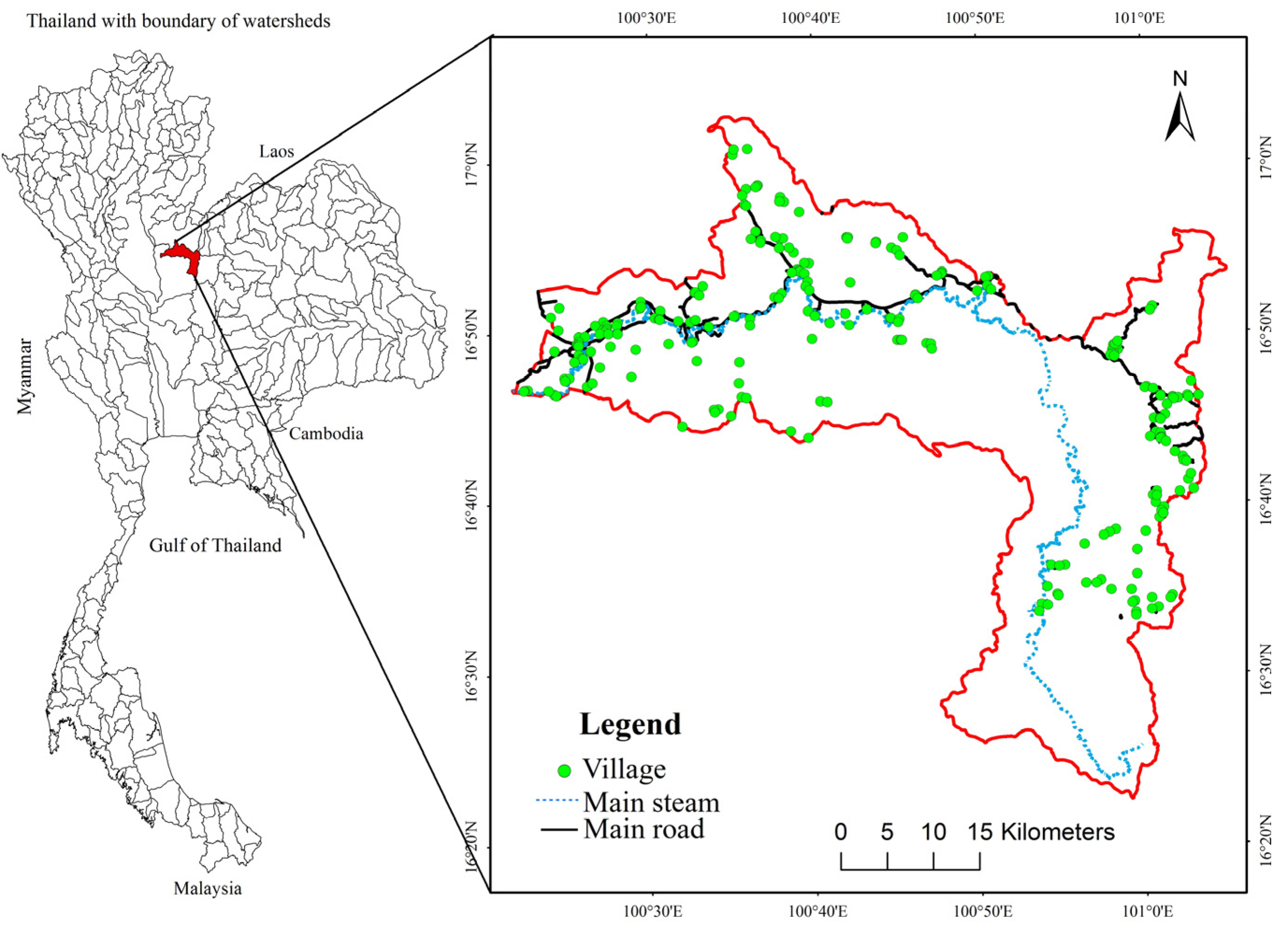
The Wang Thong watershed is situated between 16°22′10″ N and 17°2′38″ N latitude, and 100°36′10″ E to 101°3′47″ E longitude in the Wang Thong district in Phitsanulok province and Khao kho district of Phetchaboon province in northern Thailand, covering 198,082 ha (Figure 1). Sedimentary and metamorphic rock are the main geological formations in the area [21], with elevations ranging from 700 to 860 meter above sea level. The Wang Thong River, the main water source in the area, originates in the Phetchabun mountains of Khao kho district and flows through Thung Salaeng Luang national park. The climate is tropical savannah (type Aw) with three distinct seasons, namely winter (November–February), summer (March–May), and rainy (June–October). The area gets an annual rainfall of 1482 mm and the average maximum temperature during summer is 31 °C.

The dominant land cover is forest, covering more than half of the watershed area. The watershed is inhabited by a population of 96,000, mostly engaged in crop farming. About 25 per cent of the watershed area is under annual crops and the rest is under perennials (mixed orchards, rubber, and eucalyptus), or composed of urban and other land uses. Corn, cassava, paddy rice, and sugarcane are the major crops of the area.

3. Method

At first, changes in land use patterns across the study area were detected using historic land use data followed by assessment of selected ecosystem services. A field survey was conducted during February 2015 to understand land use distribution and for field verification of land uses interpreted from remote sensing data. The field survey also included household-level interviews of farm households. For selecting households for interview, the villages located in dominant land use areas (large tract of specific crops) were purposely selected by overlaying land use map with village map. Interviews of a total of 60 households were conducted in selected villages to record their socioeconomic profile and farming practices specific to the dominant land uses. The methods for specific tasks undertaken in the study are described in the following subsections.

3.1. Assessing Land Use Change

Land use change was detected for three time periods by using data from 1989, 2000, 2007, and 2013. In 1989, the logging ban was implemented in Thailand, and hence this year was taken as the starting year for this study. The year 2000 represents the immediate past, before the implementation of major agricultural policy on rubber plantations in 2004. 2013 was the year with most current land use data available at the time of the study and 2007 represents the midpoint between 2000 and 2013.

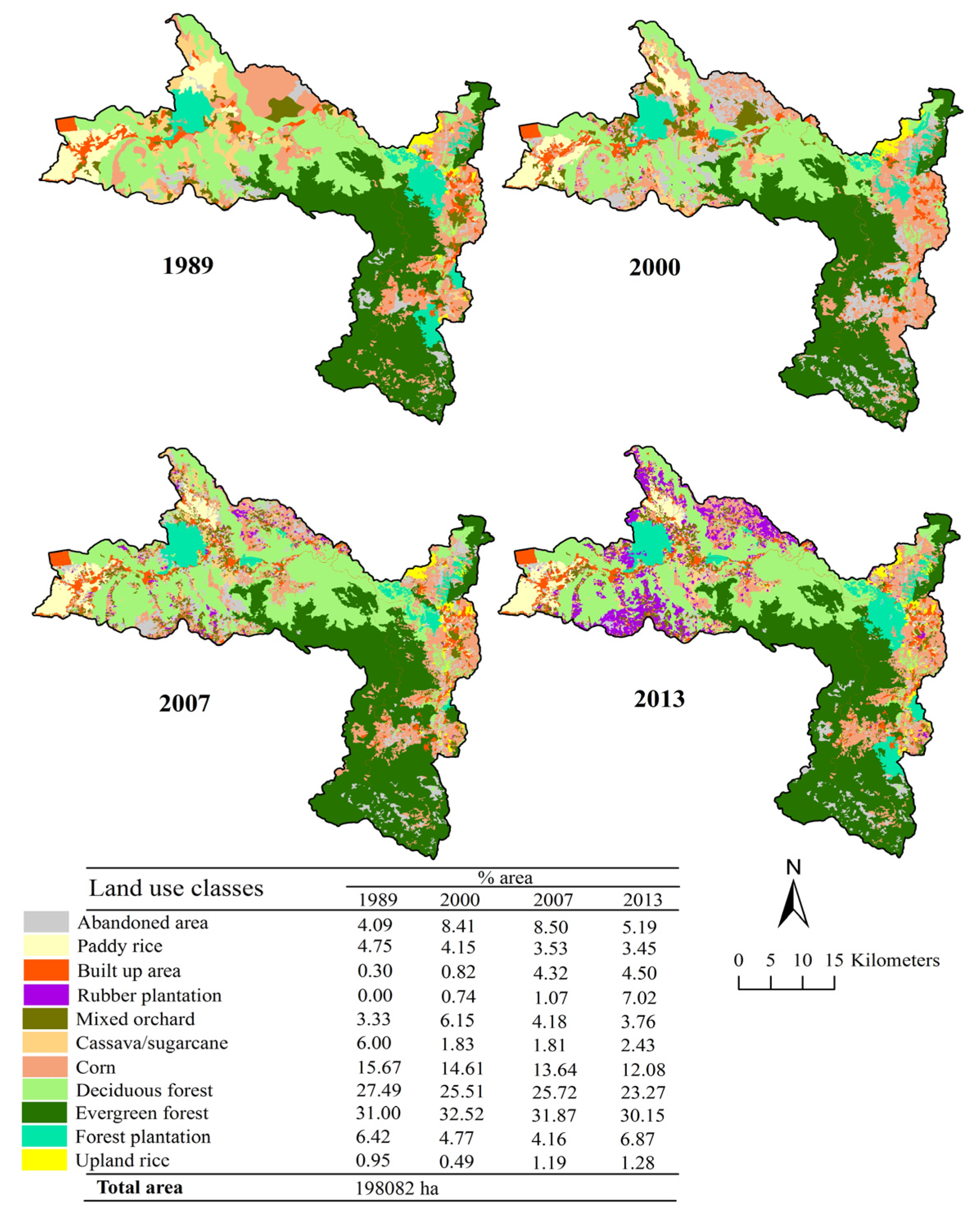
Land use maps for the years 2000, 2007, and 2013 were obtained from the Land Development Department of Thailand (LDD) in digital format (ARCGIS shape file) on request. These land use maps were interpreted from Landsat-5 Thematic Mapper (TM) satellite data and classified using the Land Cover Classification System (LCCS) at the scale of 1:50,000 and projected into a UTM zone 47N using a WGS84 or World Geodetic System 1984 for consistency. The land use classes were regrouped for all the studied years into 11 major land use classes, these were abandoned area, paddy rice, built-up area, rubber plantation, mixed orchard, cassava/sugarcane, corn, deciduous forest, evergreen forest, forest plantation, and upland rice (Figure 2).

The land use map of the year 1989 was prepared using Landsat-5 Thematic Mapper (TM) satellite data (Path 129/Row 48, 49) acquired on 25 March 1989 downloaded from the United States Geological Survey website in March 2014 (http://earthexplorer.usgs.gov/) as there was no readily available land use map for that year. The special enhancement of satellite data and the mosaicking of two scenes were accomplished using ERDAS IMAGINE 9.2 (ERDAS: Atlanta, Georgia, USA). It was difficult to tally the spectral values of two data scenes as the same feature can have different spectral values due to different atmospheric conditions if the data is taken at different times. Hence, visual interpretation of images was carried out to prepare the land use map of 1989 by digitizing in ARCGIS (version 10.2) GIS software (ESRI, Redlands, CA, USA). While interpreting the image, the 11 major land use classes present in the area were maintained to make land uses of 1989 compatible with the rest of the land use maps. Finally, changes in land use were analysed by overlaying the land use maps using ARCGIS and creating a land use change matrix.

3.2. Assessing Ecosystem Services

The Integrated Valuation of Ecosystem Services and Tradeoffs (InVEST 3.0.1) (The Natural Capital Project: Stannford, USA) tool was used to map and quantify a set of selected ecosystem services in this study. InVEST is a geospatial modelling framework tool widely used for assessing ecosystem services [22] to quantify and map a range of ecosystem services and evaluate the impact of land use change on ecosystem services [20,23]. We assessed four most important services in the watershed, namely water yield (provisioning services), sediment retention and carbon storage (regulating services), and habitat quality (supporting services), representing three major services except cultural services, as the area is not a popular tourist destination. The methods used for the assessment of each service are described below.

3.2.1. Water Yield

Water yield is the amount of water runoff from the landscape [24]. The relative water volume in a given landscape affects the quality of life in the area [25]. Consequently, changes in the landscape that affect the annual average water yield can increase or decrease land productivity. Substituting forests on slope land or mountainous areas with rubber plantations results in less water retention in the subsoil layer and reduced water discharge in the dry season due to increased evapotranspiration [26]. Conversely, in the wet season, plantations lead to larger average amounts of surface runoff and higher quantities of water loss from reduced evapotranspiration [27,28]. Consequently, an increase in water yield is prone to cause floods and landslides. In this study, water yield is considered as cumulative surface runoff measured at a specific location; hence, it is not the desired type of regulation of water flow with regards to yield and quality. In other words, observed higher water yield is an ecosystem disservice as surface runoff is dependent on vegetation cover under a given land use; thus higher runoff is not a desirable situation as an ecosystem service.

Table 1. Input data to assess water yield.

Input Data	Description/Unit	Format	Source
Precipitation	Average annual precipitation/mm·year−1	GIS raster	Thai Meteorological Department (TMD)
Reference evapotranspiration	Average annual reference evapotranspiration/mm	GIS raster	Food and Agriculture Organization (FAO)
Plant evapotranspiration coefficient	Plant evapotranspiration coefficient for each land use class	Decimal number (0–1.5)	(www.fao.org)
Root restricting layer depth	Soil depth at which root penetration is strongly inhibited because of physical or chemical characteristics/mm	GIS raster
Land use/land cover	Land use map		LDD (ldd.go.th)
Watersheds	Watershed boundary	GIS vector
Root depth	Maximum root depth for vegetated Land use classes/mm	Tabulated data	Soil map
Subwatershed	Subwatersheds within the main watersheds	GIS vector	Generated from ArcSWAT
Seasonality factor (Z)	Seasonal distribution of precipitation	Integer number (1–20)	Tallis et al., 2011
Plant available water content	Fraction of water that can be stored in the soil profile that is available for plant’s use/mm	GIS raster	Saxton and Rawls (2006)

presents the input data used in this study. All input data were converted to raster maps with a resolution of 30 × 30 meters. The FAO Penman–Montieth equation, which is based on decadal/monthly climatic data (minimum and maximum air temperature, relative humidity, hours of sunshine, and wind speed) in CROPWAT 8.0 model (FAO: Rome, Italy) was used to compute reference evapotranspiration (ETo). The information on land use change was prepared by interpreting land use maps as described in Section 3.1. Other information on root restricting layer depth, plant available water content (PAWC), watershed boundary, and soil depth were obtained from the LDD. The equation [29] was used to calculate the PAWC based on soil texture and organic matter content.

A gridded map is required for water yield model, which estimates the quantity of water runoff from each subwatershed. The model determines the amount of water running off each pixel as the precipitation, less the fraction of the water that undergoes evapotranspiration. Based on the Budyko curve developed by [30], annual water yield (Y(x)) for each pixel on the landscape (x) was calculated as follows:

$$Y\left(x\right)=\left(1-\frac{AET\left(x\right)}{P\left(x\right)}\right)·P\left(x\right)$$

(1)

where $AET\left(x\right)$ is the annual actual evapotranspiration on pixel x and $P\left(x\right)$ is the annual precipitation on pixel x.

For vegetated land use, the evapotranspiration partition of the water balance, $\frac{AET\left(x\right)}{P\left(x\right)}$, is based on an expression of the Budyko curve proposed by [31] and [30]:

$$\frac{AET\left(x\right)}{P\left(x\right)}=1+\frac{PET\left(x\right)}{P\left(x\right)}-[1+{{\left(\frac{PET\left(x\right)}{P\left(x\right)}\right)}^{\mathsf{\omega }}]}^{1/\mathsf{\omega }}$$

(2)

where $PET\left(x\right)$ is the potential evapotranspiration and $\mathsf{\omega }$ is non-physical parameter that characterizes the natural climatic-soil properties. Potential evapotranspiration $PET\left(x\right)$ is calculated as:

$$PET\left(x\right)=K_c\left(l_x\right)·E{T}_0\left(x\right)$$

(3)

where ET₀(x) is the reference evapotranspiration from pixel x and $K_c\left(l_x\right)$ is the plant (vegetation) evapotranspiration coefficient associated with the LU/LC $l_x$ on pixel x. The $\mathsf{\omega }\left(x\right)$ is an empirical parameter expressed as a linear function of $\frac{AWC\times N}{P}$, where N is the number of annual events, and AWC is the measure of water available to plant cover. The InVEST model adopts the equation given by [32] as follows:

$$\mathsf{\omega }\left(x\right)=Z\frac{AWC\left(x\right)}{P\left(x\right)}+1.25$$

(4)

where Z is the Zhang coefficient, defined as a parameter for the characterization of natural climate-soil properties. In this study, the Zhang coefficient was assigned as 4, as recommended by [24] for a tropical watershed. The 1.25 term is the minimum value of $\mathsf{\omega }\left(x\right)$, which can be seen as the value when the root depth is 0, as explained by [32], and the value of $\mathsf{\omega }\left(x\right)$ is capped to a value of 5 [32,33].

3.2.2. Sediment Retention

Sedimentation is a natural process that contributes to the health of natural habitats, but in excess it can lead to harmful outcomes [22]. Vegetation provides a vital regulating service by preventing soil erosion, but land use change usually leads to loss of vegetation cover. Sedimentation is caused by soil erosion resulting from the deterioration of a watershed, manifested as greater sediment deposits [34], and hence, prevention of soil erosion or increased sediment retention is regarded as an ecosystem service. Sediment retention not only preserves soil fertility but also maintains water quality [35]. The degree of sediment that rivers deposit is significant in determining the way the watershed system behaves for several reasons including its influence on material flux, geochemical cycles, water quality, changes in the morphology of water channels, patterns of delta development, and the aquatic habitats.

For the landscape manager, it is essential to grasp the ways in which sediment retention preserves certain services in a natural landscape. For example, stakeholders need to take into account the source of sediment production and ultimate deposition so that they can develop plans to limit sediment loads in watershed areas. Equipped with this knowledge of local sediment dynamics, they are able to focus on maintaining areas capable of greater sediment retention or areas of low impact for agricultural cultivation [36]. The resource managers can plan to mitigate the impact of agricultural activities if they understand that the fact that different types of land management strategies cause non-linear impacts [37].

The sediment retention module in the InVEST uses the Universal Soil Loss Equation (USLE) developed by [38] at the grid scale together with a sediment retention approach for sediment deposition. The information on land use pattern, rainfall, soil characteristics, and topography was prepared at grid i level to estimate soil erosion as:

$$USL{E}_i={(R.K.LS.C.P)}_i$$

(5)

where R is the rainfall erosivity factor (MJ mm/ha/year), K is the soil erodibility factor (MJ mm/ton/ha), LS is the topographic factor, C is the crop management factor, and P is the conservation practices factor. Using those factors, the sediment retention is computed as follows:

$$R_i.K_i.L{S}_i\left(1-C_i{P}_i\right)SD{R}_i$$

(6)

where $SD{R}_i$ is the proportion of soil loss actually reaching the watershed outlet for pixel i.

The data and their sources used to compute sediment retention are summarized in

Table 2. Input data to assess sediment retention.

Input Data	Description	Format	Source
Rainfall erosivity	An erosivity index value for each cell	GIS raster	TMD
Digital Elevation Model (DEM)	An elevation value for each cell	GIS raster	LDD
Soil erodibility	A soil erodibility value for each cell	GIS raster	LDD
Land use	An integer land use code for each cell	GIS raster
Watershed	Watershed contributes to a point of interest where water quality will be analysed	GIS vector	LDD
USLE C factor	Cover management factor for USLE, a floating point value between 0 and 1	Tabulated value	LDD
USLE P factor	Support practice factor for USLE, a floating point value between 0 and 1	Tabulated value	LDD
Threshold flow accumulation	Number of upstream cells that must flow into a cell	Model input	Sharp et al., 2015

.

3.2.3. Carbon Storage

Carbon stock is an important indicator of the potential capacity of land to hold carbon. Change in carbon stock may have direct consequences on the socioeconomic wellbeing of local communities and also on biodiversity [39]. The InVEST model assesses total carbon stock in land under a variety of use. For each land use, the estimates of carbon pool, namely dead organic matter, above and belowground biomass and soil organic matter in soil are needed [16,20,40,41] to subsequently put into the land use maps and then create an integrated map showing the carbon stock contained in each cell. Thus, the net change in carbon stock overtime can be computed using historical land use maps. In the model, a given map grid that has not undergone land use change retains a sequestration and loss value of 0 over time. In this study, the biomass carbon stock for each land use type was not measured. Instead, we compiled and used available secondary biomass carbon rates from several local studies (

Table 3. Carbon stocks (ton/ha) for different land use types.

Land Use Types	Above Ground	Below Ground	Soil	Dead Organic Matter	Total
Abandoned	16.0 c	30.0 c	30.0 c	13.0 c	89.0
Paddy rice	3.0 c	2.0 c	10.0 c	4.0 c	19.0
Built-up	5.0 c	10.0 c	16.0 c	2.0 c	33.0
Rubber plantation	12.1 a	6.0 a	66.0 b	12.0 c	96.1
Mixed orchard	65.0 c	40.0 c	25.0 c	6.0 c	136.0
Cassava/sugarcane	3.0 c	2.0 c	10.0 c	4.0 c	19.0
Corn	3.0 c	2.0 c	10.0 c	4.0 c	19.0
Deciduous forest	64.9 a	32.4 a	172.0 b	34.7 c	304.0
Evergreen forest	112.5 b	32.7 b	238.0 b	43.4 c	426.6
Forest plantation	19.0 e	7.4 e	66.0 e	12.0 c	104.4
Upland rice	3.0 c	2.0 c	10.0 c	4.0 c	19.0

Note: ^a, ^b, ^c, ^d, ^e refer to source of information; ^a: [42], ^b: [43], ^c: [44], ^d: [45], ^e: [46].

).

For estimating carbon stocks, the model needs land use map in standard GIS raster format and carbon pools table in *.csv or *.dbf file. These two inputs must match in the code column of each other. The values of each carbon pool were encoded in land use maps using the following equation.

TotCar = Σ (CAg_i × A_i) + (CBg_i × A_i) + (CSl_i × A_i) + (CDo_i × A_i),

(7)

where TotCar = Total amount of carbon; CAg_i = Average amount of carbon stored in above ground with Land use _i; CBg_i = Average amount of carbon stored in below ground with Land use _i; CSl_i = Average amount of carbon stored in soil with LU/LC _i; CDo_i = Average amount of carbon stored in dead organic matter with Land use _i; A_i = Size of Land use _i.

3.2.4. Habitat Quality

Habitat quality can be defined as a terrain’s ability to maintain appropriate conditions for the viability of organisms [24]. The InVEST model takes a habitat-based perspective, where the quality and singularity of habitat serve as proxies for biodiversity. For a habitat to be considered of high quality, it must be undisturbed and function within the bounds of past variability. Thus, it is assumed that habitat quality deteriorates proportionately to the rate of increase in human influenced land use [24], after [47]. Quality of habitat is also vulnerable to a variety of threats, to which it will have relative degrees of sensitivity, as well as to the gaps between healthy habitat zones and relative proximity of protected zones and sources of threats. The InVEST model determines the impact i_rxy of threat r from grid cell y on habitat in grid cell x, by employing both exponential and linear decay functions, while considering distances of threat sources from a given habitat, as seen in the equations below:

$$i_{rxy}=1-\left(\frac{d_{xy}}{d_{r\text{ max}}}\right)\text{ if linear}$$

(8)

$$i_{rxy}=exp\left[-\left(\frac{2.99}{d_{rmax}}\right)d_{xy}\right]\text{ if exponential}$$

(9)

where d_xy is the linear distance between grid cells x and y d_rmax is the maximum effective distance of the threat. The total threat level D_xj in a grid cell x with land use j is then calculated as

$$D_{xj}={{\displaystyle \sum }}_{r=1}^R{{\displaystyle \sum }}_{y=1}^{Y_r}\left(\frac{w_r}{{{\displaystyle \sum }}_{r=1}^R{w}_r}\right)r_y{i}_{rxy}{\mathsf{\beta }}_x{S}_{jr}.$$

(10)

Habitat quality Q_xj of land use j is determined from the degree of habitat suitability of land use j as

$$Q_{xj}=H_j\left(1-\left(\frac{D_{xj}^z}{D_{xj}^z+k^z}\right)\right).$$

(11)

The model requires five types of input data (

Table 4. Input data used to assess habitat quality.

Input Data	Description	Format	Source
Current land use map	Land use land cover map	GIS raster	LDD
Threats data	A table containing information on each threat’s relative importance or weight and its impact across space.	Tabulated data	Expert knowledge and field observation
Sources of threats	Distribution and intensity of each individual threat	GIS raster	Generated from ArcMap
Habitat types and their sensitivity to each threat	A table of land use type containing habitat suitability scores and weights of sensitivity	Tabulated data	Expert knowledge and literature review
Half-saturation constant	Value of parameter k in equation. The choice of k determines the spread and central tendency of habitat quality scores.	Model input	Preliminary run of the model

), and runs using a grid map by assigning each grid cell a land use type. In this study, four threats, namely agricultural areas, urban areas, paved roads, and dirt roads were considered to assess habitat quality. For agricultural areas, the risk of habitat degradation was calculated as a combination of the effects of rate of erosion, the likelihood of pollution from pesticides and physical variations in upland flora and insects. Urban or developed areas were a threat to the health and quality of habitat as they cause either destruction or fragmentation of natural habitats due to the construction of roads, houses, and industry, resulting in biodiversity loss. Small habitat patches persisting due to fragmentation are unable to support the same level of genetic or taxonomic diversity [48].

In the dearth of information on biodiversity, we modelled general terrestrial biodiversity by considering the disturbed vegetation areas as non-habitat and undisturbed areas as habitat. The main causes of habitat deterioration were assigned degrees of impact and integrated with a maximum distance of degradation effect to map the degree to which each land use affected the quality of the habitat. The evaluation of the amount of effect of each habitat type on degradation was determined according to principle concepts of landscape ecology and conservation biology [49,50] specific to each degree of biodiversity. Sensitivity scores were calculated based both on methods common in the research literature [24,51] and expert knowledge. To determine the sensitivity scores of threats and habitat types, we interviewed six key informants to get information on the area and historical background of the community including physical factors and socioeconomic and cultural data. The key informants were government officials of the Royal Forestry Department, the Faculty of forestry of Kasetsart University, and village leaders. The sensitivity scores are given in Appendix A.

3.2.5. State of Ecosystem Services

For an integrated assessment, the ecosystem services at a particular location were computed as an index (unitless value) by combining the four services for the year 2013 to generate a suite of indices. We first reclassified the range of values of each service into five classes (very low, low, moderate, high, and very high). The three ecosystem services (soil retention, habitat quality, and carbon stock) were reclassified and coded as having a value of 1 (very low ecosystem service), 2 (low), 3 (moderate), 4 (high), or 5 (very high). For water yield, the lowest value of 1 was coded as having a very high ecosystem service and a value of 5 as low. This is because the increase in water yield is not considered a positive ecosystem service for the reasons discussed in Section 3.2.4. Then all reclassified maps were overlaid to produce a map showing the state of ecosystem services for the year 2013.

The ecosystem service indices were assessed at the position of the pixel and then combined at subwatershed and watershed level in the study years (1989, 2000, 2007, and 2013) to juxtapose ecosystem services in space and time. In order to evaluate the ecosystem services’ rate of change over time, we mapped and determined the state of ecosystem services (ESi), depending on time and location variables that quantify a specific ecosystem service at one specific time i. As suggested by [51], the degree of variation in each individual ecosystem service with respect to its past state was determined as in Equation (12):

$${\text{ESCI}}_x=\left[\frac{{\text{ES}}_{\text{CUR}xj}-{\text{ES}}_{\text{HIS}xi}}{{\text{ES}}_{\text{HIS}xi}}\right]$$

(12)

where ESCI_X represents the Ecosystems Services Change Index of service x, ${\text{ES}}_{\text{CUR}x}$ and ${\text{ES}}_{\text{HIS}x}$ represent the current and historic state of ecosystem service values of service x at times j and i, respectively. The ESCI represents the relative gain or loss of each particular ecosystem service, in a scale from minus 1 to plus 1 with 0 showing no ES change. Minus 1 means a loss of all services and plus 1 indicates a gain of all services.

4. Results

4.1. Land Use Change

Forest is dominant in the study area. The agricultural land use type consisted of cassava, paddy rice, upland rice, sugarcane, corn, and mixed orchard. Corn was the most common crop in the area. The classified land use map and the percentage area under all 11 land use classes for 1989 to 2013 are presented in Figure 2. In the first period (1989–2000), forests, particularly deciduous and plantation, continued to decrease in extent, along with upland crops (cassava, sugarcane). Abandoned areas, built-up areas, and mixed orchards increased during this period. The study area did not have rubber in 1989 and, by 2000, 0.74% of the watershed was occupied by rubber cultivation. During the second period (2000–2007), forests (evergreen and plantation) continued to decline slightly. Mixed orchard also declined, while there was a rapid increase in built-up areas (from 0.82% to 4.32% of watershed), rubber plantations, and upland rice areas. Forest had been converted to agricultural area (mixed orchard, corn) and eventually farmers replaced their fields with commercial rubber plantations. During the third period of investigation (2007–2013), forests (evergreen and deciduous) continued to decrease although plantation forest increased slightly as a result of an effort to rehabilitate the degraded forests influenced by the forest enactment law and increasing awareness about the importance of forest conservation. Similarly, areas under mixed orchard and corn cultivation, were also found to have decreased whereas built-up areas, cassava, sugarcane, and upland rice agricultural areas had increased slightly. The most notable change during the whole study period was the increase in area of rubber plantations from 0% to more than 7% (14,000 ha) of the watershed area. Similarly, built-up areas also increased by about 4% during the study period. Most of the increase came from the decrease of forests and some upland crop areas.

The major proportions of land use in the study area were forest (deciduous, evergreen, and forest plantation) and agricultural land (corn and cassava). Based on the household survey, rice was commonly grown as a subsistence crop by 58% of surveyed households, however the total area under rice cultivation does not account for more than 10% in areal coverage as rice farming is in small scale. Areas under corn cultivation are still larger than the total area under rice cultivation as they are mostly large-scale operations pursued by relatively few farmers (23% of surveyed households). Rubber cultivation was found to have grown rapidly compared to the past. At present, some 25% of households cultivate rubber in the area, which is more than the percentage of households cultivating corn. Until two decades ago, a majority of farmers grew rice and corn and used to alternate these two crops for higher productivity. In recent years, paddy and corn cultivation have been reduce in favour of rubber cultivation.

4.2. Ecosystem Services

4.2.1. Water Yield

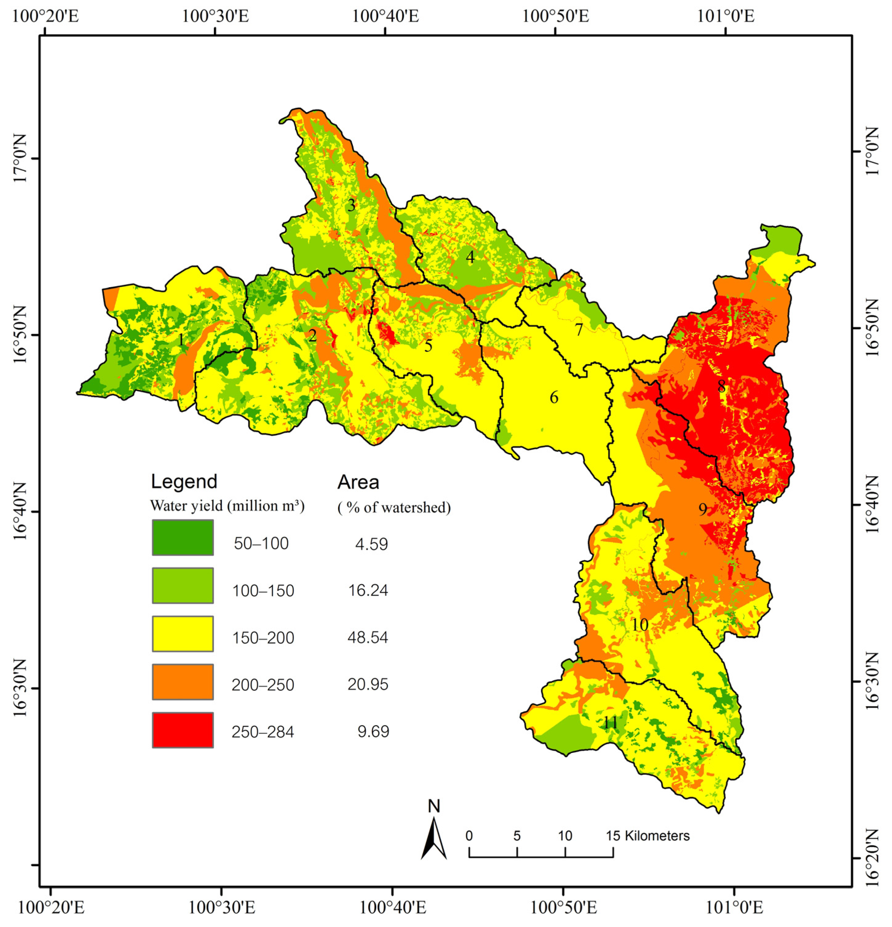
The model results for water yield computation were aggregated into each subwatershed and subsequently the entire study area was mapped out for spatial variation of water yields. Of 11 subwatersheds in the study area, the computed water yield at subwatershed level ranged from 50 to 284 million m³ (Figure 3). About 49% of the study area has a water yield within the range of 150 to 200 million m³, while 21%, 16%, 10%, and 5% of the study area had a water yield in the range of 200–250, 100–150, 250–248, and 50–100 million m³, respectively.

The results for water yield generated for each subwatershed showed a higher water yield volume for subwatersheds 8 and 9, which have relatively more area under upland agriculture. Subwatersheds 1, 4, 5, 6, and 7 generated comparatively lower water yield than subwatersheds 2, 8, 9, 10, and 11. Subwatershed 8, located in the northeast, had the highest water yield (284.19 million m³) as it has the largest area dominated by agriculture (4.94%), followed by subwatershed 9 (2.49%).

4.2.2. Sediment Retention

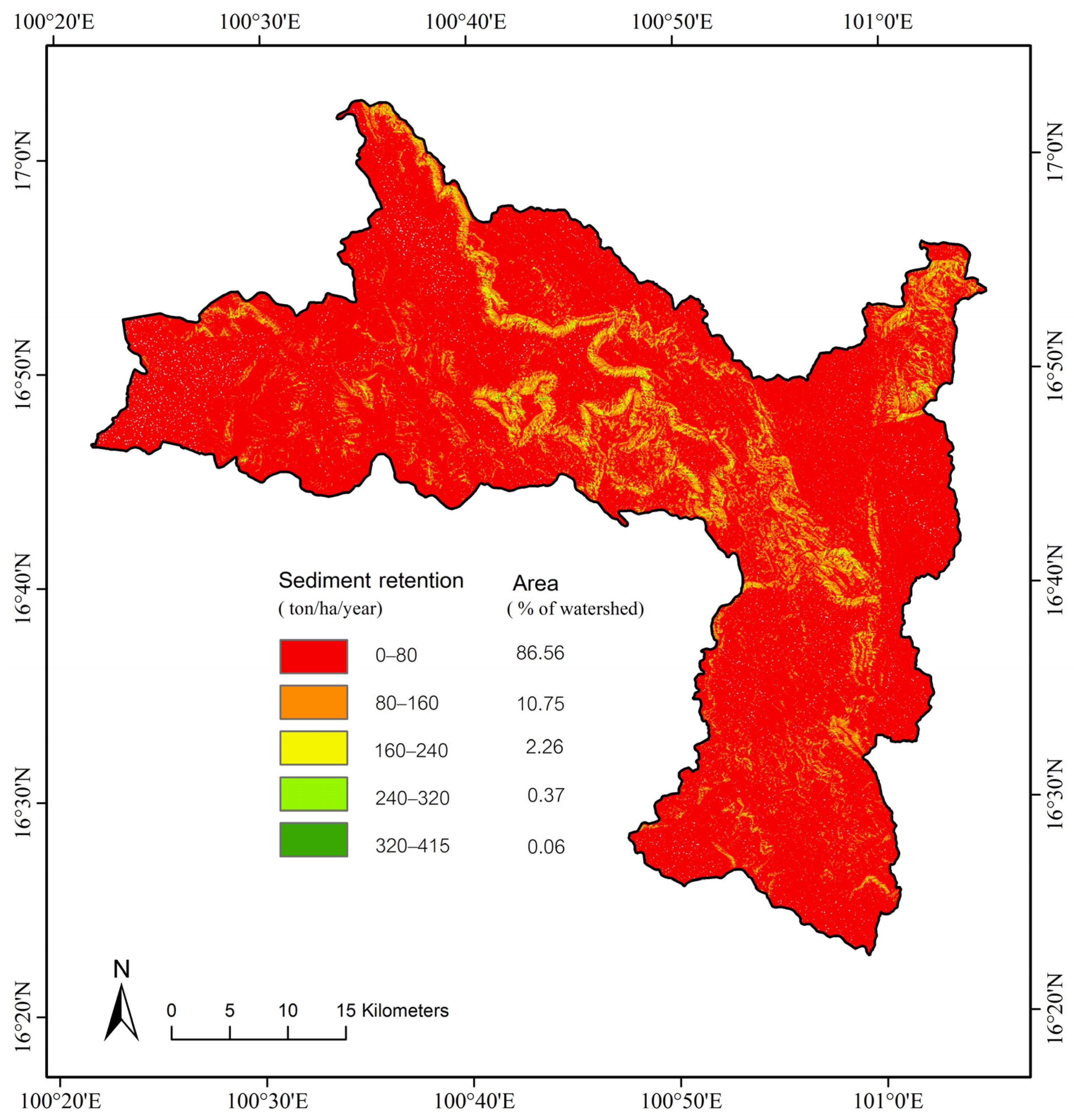
Sediment retention is influenced by the extent and type of vegetation of a given unit of land. The computed average sediment retention for the whole study area was 189 ton/ha/year. We categorized the observed sediment retention (0–415 ton/ha/year) into five classes, namely very low (0–80 ton/ha/year), low (80–160), moderate (160–240), high (240–320) and very high (320–415 ton/ha/year). The class limits were decided for the observed retention in the study area, not considering any other threshold, as the purpose was to identify the areas with highest and lowest retention within a watershed.

It was observed that the majority of the area (86.5%) has very low sedimentation retention, as shown in Figure 4, indicating higher soil loss in the watershed. Nearly 11% of the watershed area has low retention and the rest of the area (<3%) has moderate to very high retention.

4.2.3. Carbon Storage

The carbon densities in terrestrial land cover decreased during the period of the study due to the higher rate of transition from natural to cultivated land use as result of human influence. The observed carbon density in the study area was highest in evergreen forest areas (427 ton/ha), followed by deciduous forest (304 ton/ha), while the lowest carbon storage level was in croplands, like paddy rice, cassava/sugarcane, corn, and upland rice (19 ton/ha). Figure 5 shows the distribution of carbon stock in the study area and the percentage of area in each range of carbon stock. The highest range in the entire area was 340–427 ton/ha carbon stock, covering 30.15% of the watershed area. About 23% of the area had 0–85 ton/ha carbon stock. Similarly, 23% had 85–170 or 255–340 (ton/ha) carbon stock.

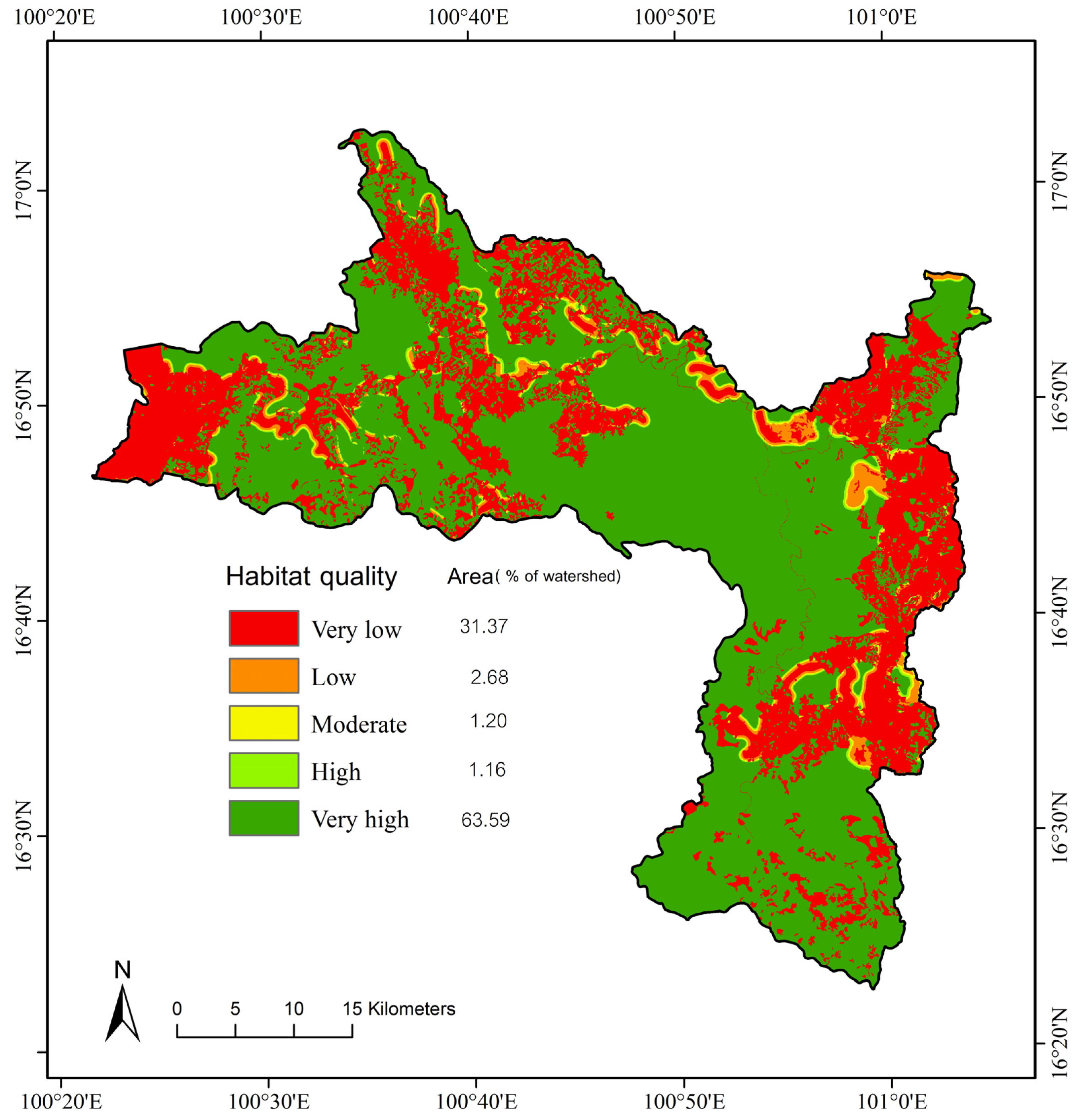
4.2.4. Habitat Quality

Habitat quality and degradation classes in this study were defined as degradation and loss of natural habitats, which is a major cause of biodiversity loss [52]. The InVEST model results differentiate habitat quality in terms of proportion of area in the watershed by summarizing the aggregate scores of all grid cells. This is based on the coefficient of variation of the average scores across the study area obtained from expert judgment and through the literature review. Higher aggregate habitat quality scores imply a greater amount of habitat area, which is a good indicator of biodiversity. Severity is relative to each area, hence the computed habitat quality classes were categorized into five classes: very low (0–0.2), low (0.2–0.4), moderate (0.4–0.6), high (0.6–0.8), and very high (0.8–1.0).

Forested areas in the watershed had a higher habitat quality than the areas under agriculture and settlement (Figure 6). Of total habitat quality in the watershed, the forested area (deciduous and evergreen) comprises about 74% of the existing habitat quality, while agricultural area (paddy, cassava/sugarcane, corn, and upland rice) comprises only 5%.

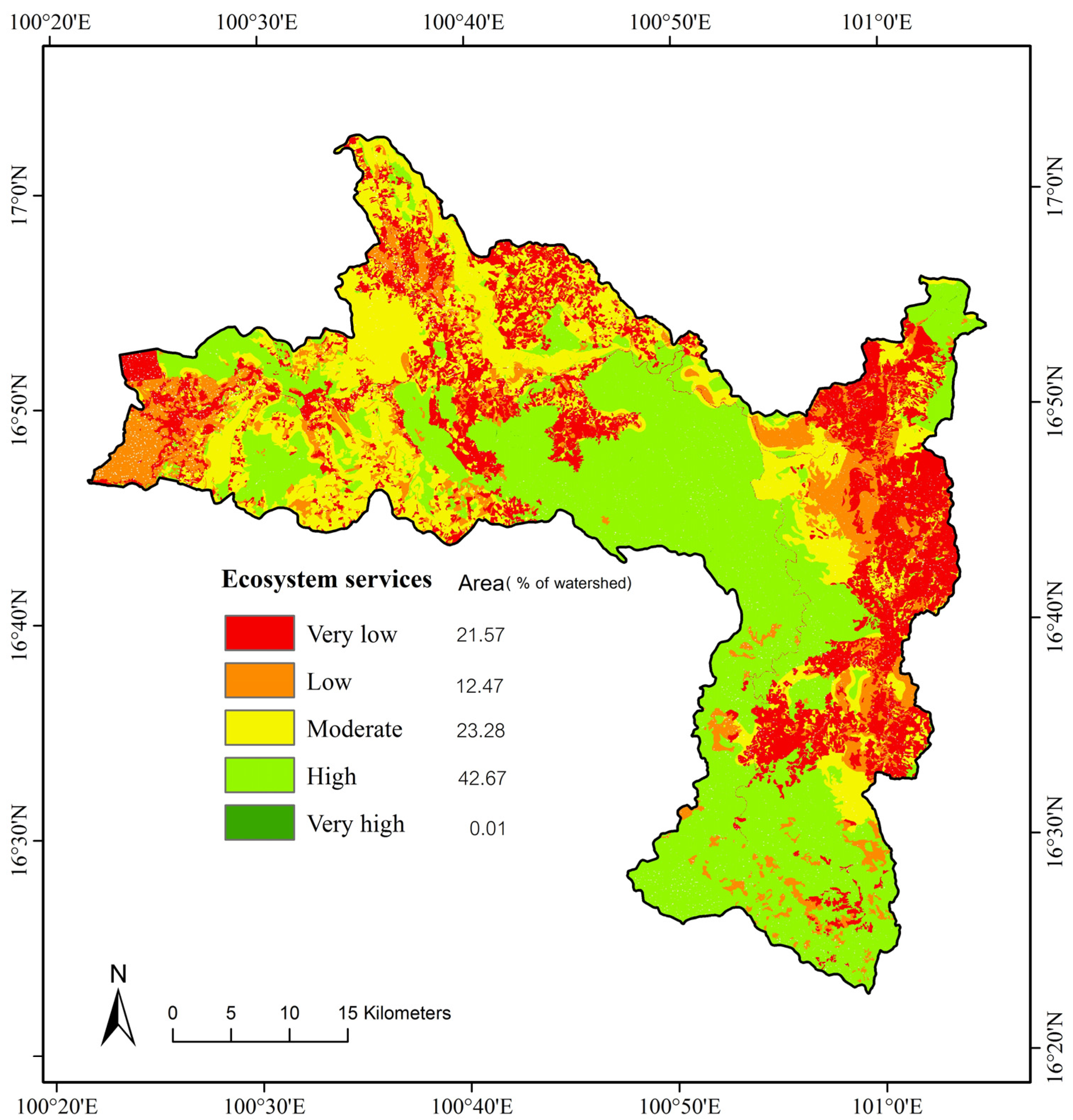
4.3. Impact of Land Use on Ecosystem Services

The overall ecosystem service (ES) was assessed by combining the index of four different services, namely water yield, sediment retention, carbon storage, and habitat quality, as discussed above. Figure 7 shows that there was no area that could be considered to have very high ecosystem services. It is to be understood, however, that a very high level of ecosystem services is contextual in the case of the study area, referring to a land unit with the best condition of all four services being investigated. Nearly 43% of the area was found to have a high degree of ecosystem services, whereas 23% was moderate and another 35% of the area had low to very low ecosystem services.

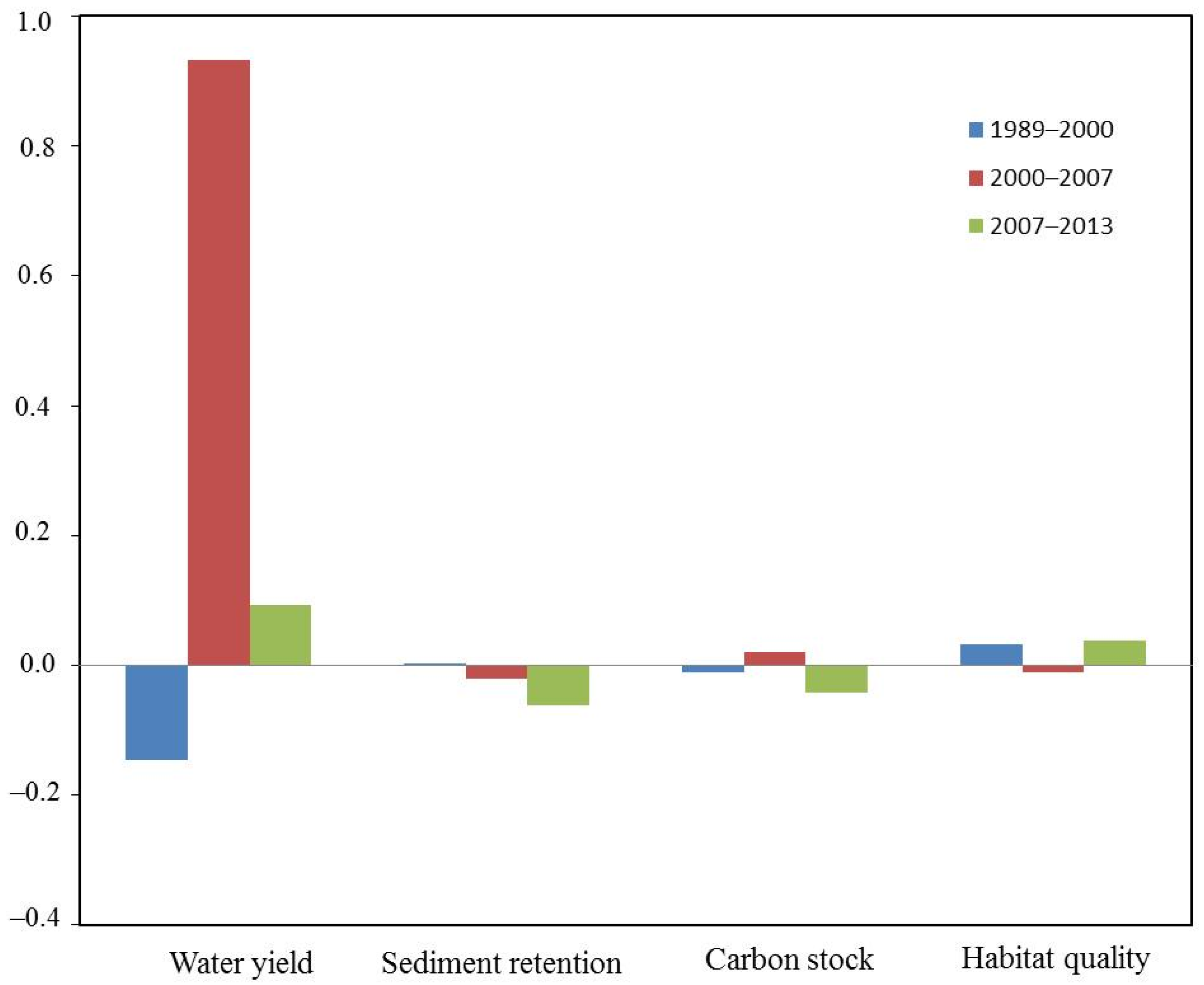
For the three periods under investigation (1989–2000, 2000–2007, and 2007–2013), an increasing trend was observed in general for water yield and habitat quality and vice versa for sediment retention and carbon storage. Water yield was found to have increased more during 2000–2007 with an ESCI of 0.93 compared to that during 2007–2013 (ESCI = 0.09) (Figure 8). Minus 0.18 ESCI indicates that water yield decreased slightly during 1989–2000. The habitat quality decreased from 0.03 ESCI during 1989–2000 to −0.01 (2000–2007), but increased to 0.04 during 2007–2013. In contrast, sediment retention gradually decreased in the periods 1989–2000, 2000–2007, and 2007–2013, as the computed ESCI were 0.0, −0.02, and −0.06, respectively. The overall status of all the services ranged from −0.15 to 0.03 for the year 2000, −0.01 to 0.93 for 2007, and −0.06 to 0.09 for 2013.

Table 5. Percentage of each ecosystem service for each land use class (1989–2013).

Year	Land Use Class	% of Ecosystem Service in Land Use Class
		Water Yield	Sediment Retention	Carbon Storage	Habitat Quality
1989	Abandoned	7.3	0.4	1.5	0.0
	Paddy rice	6.4	0.1	0.4	1.3
	Built-up	15.5	0.0	0.1	0.0
	Rubber plantation	0.0	0.0	0.0	0.0
	Mixed orchard	6.9	0.2	1.9	4.4
	Cassava/sugarcane	9.4	0.2	0.5	1.7
	Corn	24.5	4.7	1.3	4.6
	Deciduous forest	16.1	46.3	35.4	34.3
	Evergreen forest	8.9	46.7	56.0	45.4
	Forest plantation	2.7	1.4	2.8	8.0
	Upland rice	2.3	0.0	0.1	0.3
2000	Abandoned	9.8	0.9	3.2	0.0
	Paddy rice	4.5	0.0	0.3	1.1
	Built-up	18.0	0.1	0.1	0.0
	Rubber plantation	1.0	0.1	0.3	0.8
	Mixed orchard	9.2	0.4	3.6	7.6
	Cassava/sugarcane	3.8	0.1	0.1	0.5
	Corn	21.1	4.3	1.2	4.1
	Deciduous forest	9.3	38.4	42.4	34.6
	Evergreen forest	6.9	54.7	46.6	45.5
	Forest plantation	15.0	1.0	2.1	5.7
	Upland rice	1.4	0.0	0.1	0.1
2007	Abandoned	14.2	0.9	3.2	0.0
	Paddy rice	4.5	0.0	0.3	1.0
	Built-up	15.7	0.3	0.6	0.0
	Rubber plantation	2.5	0.1	0.4	1.3
	Mixed orchard	14.7	0.3	2.4	5.4
	Cassava/sugarcane	3.9	0.1	0.1	0.5
	Corn	20.1	4.1	1.1	3.9
	Deciduous forest	13.9	44.2	32.9	36.9
	Evergreen forest	6.4	49.0	57.1	45.6
	Forest plantation	1.7	0.9	1.8	5.1
	Upland rice	2.4	0.1	0.1	0.3
2013	Abandoned	10.6	0.6	2.0	0.0
	Paddy rice	4.1	0.0	0.3	0.9
	Built-up	15.0	0.3	0.6	0.0
	Rubber plantation	9.7	1.1	3.0	7.6
	Mixed orchard	14.5	0.3	2.2	4.6
	Cassava/sugarcane	6.3	0.1	0.2	0.7
	Corn	17.9	3.9	1.0	3.4
	Deciduous forest	11.9	42.6	31.0	33.0
	Evergreen forest	5.2	49.4	56.4	41.2
	Forest plantation	2.1	1.6	3.2	8.3
	Upland rice	2.7	0.1	0.1	0.3

presents the contribution of each land use on each ecosystem service for each studied year. A great degree of fluctuation can be seen in the contribution of each ecosystem service between land uses across the study years. For 1989, the highest contribution in the total water yield at the watershed level was from land use under corn cultivation (24.5%), followed by deciduous forest (16.1%), whereas these uses were 17.9% and 11.9%, respectively, in 2013, indicating that this service has actually improved for these land uses compared to the past. On the other hand, the contribution from abandoned land, rubber plantations, and mixed orchards increased in 2013 compared to 1989, implying that these land uses have deteriorating services as far as the regulation of water flow is concerned. Similarly, of the total sediment retention, carbon stock, and habitat quality at the watershed level, forests play the most significant role out of these three ecosystem services. This is in line with many other studies, for example, [53], who stated that the zones of the La Antigua watershed in Mexico with ample forest cover had better quality ecosystem services, and the study by [54], who noted a greater proportion of five ecosystem services in land use categories with undisturbed old-growth vegetation and on somewhat deteriorated animal grazing land.

5. Discussion

Land use change in the Wang Thong watershed has undergone a typical trajectory from forest conversion to agricultural area (mixed orchard, corn) for subsistence purposes and eventually to commercial crops (rubber plantation). The built-up area, which was less than 1% in 1989, had increased to more than 4% by 2013. This, however, is a general trend elsewhere due to population growth and increasing urban economic activity. The northern region of Thailand is one of the major forested areas compared to other parts of the country. At present, it contains more than half of the country’s forests. The region had 118,000 km² of forests in 1961, which declined to 80,000 in 1989, 74,000 in 1998, and 88,000 in 2006 [55]. This massive deforestation for commercial purposes, along with rapid forest and environmental degradation in the country, prompted the government to institute a logging ban in all forests in 1989. This shows that despite the promulgation of law, forested areas have continued to decline and it is only recently that some improvement has been seen, mainly due to increased efforts to replant forests and conservation.

With regard to agricultural land (mostly dominated by corn and rice), while the area devoted to paddy rice (flooded rice) has decreased slightly over the years, rubber cultivation was found to have rapidly increased compared to the past. Up until two decades ago, the majority of farmers grew rice and corn and used to alternate between these two crops to achieve better production. In recent years, there has been a trend to reduce paddy and corn cultivation while increasing rubber tree cultivation.

Many factors function to impact water yield through land use, the most significant of which are plant cover affecting evapotranspiration, the soil’s water infiltration and retention capacity, and the degree to which plant cover can capture moisture to be transferred into soil. While land uses having with higher evapotranspiration potential result in an increase in surface runoff, decreased forest cover also leads to greater water yield [56,57]. The effects however depend to a large extent on the way in which the land is utilized. With regard to water yield in the study period, a significant increase in annual water yield between 2000 and 2007 was observed, mainly due to an increase in built-up areas and upland rice cultivation and decreased deciduous forest area cover during this period, as classified from land use type compared to the years 1989 and 2013. Similar findings reported in other studies [58,59,60] show that urbanization has an impact on flooding due to higher levels of runoff. Agricultural areas mostly under annual crops have had a greater impact on surface runoff and thus water yield compared to natural forest cover, which usually produces less runoff. Plantation forest, such as rubber, did not show specific trends affecting water yield when considering the total water yield of the watershed, probably due to the turnover of the rubber areas as they keep on changing due to some areas harvested and new areas are planted.

The tendency for decreased sediment retention over the study period indicates increasing soil erosion due to the major land use changes discussed earlier. A relatively higher rate of sediment retention was observed, mostly in the case of evergreen and deciduous forest. The lowest retention rate was associated with agriculture, especially upland area cultivation of sugarcane/cassava, which has a high slope, as observed during the field survey also. In addition, no management practices, such as terracing, are practiced in the area. Decreased soil retention was due to the use of abandoned areas and other agricultural areas for rubber or orchard plantation when the soils are disturbed, leading to increased erosion and low sediment retention.

The results of assessment of carbon stock depend greatly on the accuracy and reliability of estimates of carbon stock for a given land use type [61]. Although it is a challenge to produce accurate estimates due to several factors including seasonal fluctuation, InVEST model uses absolute values for simplified results not considering seasonal fluctuation and feedback mechanism [24,62]. Nonetheless, the model result is still meaningful in relative terms as it allows for comparison of biomass and soil carbon stock in different land use categories and makes it possible to quantify losses in carbon stock. However, the carbon module does not include the total carbon load, nor does it account for the variability of carbon stock depending on any particular land use type [24]. This is partly due to changes in some land use types, particularly annual crops (e.g., rice, corn) within a yearly timeframe, and changes in physiological processes in perennials influenced by seasonal variation. We observed slight decreased in carbon stock during the study period because of reduced sediment retention and increased erosion leading to loss of carbon stock. A reduction in aboveground biomass resulting from the relative decrease in forested areas during 2007–2013 also caused a reduction in carbon stock.

Habitat quality is related to characteristics of the natural landscape. The study area has a national park, where habitat quality is maintained due to the presence of natural landscape compared to some other watersheds in the region, which do not have any designated protected areas. The overall ecosystem services in the watershed are satisfactory since nearly 43% of the watershed was found to have an above-average condition. Given the specific biome in any region, it is hard to compare the overall ecosystem services of one place to another. It is also difficult to establish a threshold class of ecosystem services as ecosystems naturally differ in different locations. Hence, it is to be noted that different categories of ecosystem services and their spatial distribution in the study area represent the relative condition of each ecosystem service within the study area. The result should be useful for guiding future land use activities in the watershed by understanding which areas are relatively worse off and thus need attention for conservation planning rather than comparing with other watershed systems.

6. Conclusions

Land use change has occurred in the study area in the past 24 years due to economic development and government policy. Over the period, the areas under paddy, cassava, sugarcane, corn, and deciduous forest have decreased slightly while built-up areas and upland rice areas have increased. Changes in land use patterns brought both positive and negative impacts on ecosystem services. Negative impacts were observed in agricultural dominated areas as 80% of the watershed has an above-average water yield, implying reduced storage of soil moisture. This is mainly due to the rainfall converting to surface runoff contributing river flow, and also due to the lack of land’s ability to regulate water flow. A substantial majority of the area has very low sediment retention, indicating higher soil loss. Similarly, about half of the watershed area has below-average carbon stock and two-thirds of the watershed has above-average habitat quality. There was no area that could be considered to provide very high ecosystem services. Only two-fifths of the watershed was found to have high ecosystem services.

Land use change has influenced overall ecosystem services, with variation in the spatial distribution and temporal change in the ecosystem services. An increase in abandoned areas, built-up areas, and rubber plantations is a major concern as these land use types can lead to decreased ecosystem services. Areas under some upland crops reduced compared to the past, which is an indication of better sediment retention and carbon storage. Forests continue to decline undermining the ecosystem services in the area in spite of the logging ban and the promotion of forest plantation scheme.

The study provides the spatial distribution of each ecosystem service in the study area as valuable input to land use planning. As we used four variables to assess overall ecosystem services in our study, the results may vary if the variables are changed. Hence, it is not feasible to compare our results with those of other models. Yet, it is expected that the present study’s conclusions with respect to the spatial distribution of ecosystem services can help identify land units that are relatively worse off so that appropriate land use activities can be planned to improve the ecosystem services from these units and eventually the whole watershed.

References

- Srivastava, P.; Kumar, U. Growth in the greater Mekong subregion in 2000–2010 and future prospects. In Proceeding of International conference on GMS 2020: Balancing Economic Growth and Environmental Sustainability, Bankgog, Thailand, 20–21 February 2012; pp. 12–41.
- Minna, H. Forest conflict in Thailand: Northern minorities in focus. Environ. Manag. 2009, 43, 381–395. [Google Scholar]
- Trisurat, Y.; Alkemade, R.; Verburg, P.H. Projecting land-use change and its consequences for biodiversity in Northern Thailand. Environ. Manag. 2010, 45, 626–639. [Google Scholar] [CrossRef] [PubMed]
- Lambin, E.F.; Geist, H.J.; Lepers, E. Dynamics of land-use and land-cover change in tropical regions. Ann. Rev. Environ. Resour. 2003, 28, 205–241. [Google Scholar] [CrossRef]
- Carlson, K.M.; Curran, L.M.; Ratnasai, D. Committed carbon emissions, deforestation, and community land conversion from oil palm plantation expansion in West Kalimantan, Indonesia. Proc. Natl. Acad. Sci. USA 2012, 109, 7559–7564. [Google Scholar] [CrossRef] [PubMed]
- Wösten, J.H.M.; Clymans, E.; Page, S.E.; Rieley, J.O.; Limin, S.H. Peat–water interrelationships in a tropical peatland ecosystem in Southeast Asia. Catena 2008, 73, 212–224. [Google Scholar] [CrossRef]
- Bosselmann, A.S. Mediating factors of land use change among coffee farmers in a biological corridor. Ecol. Econ. 2012, 80, 79–88. [Google Scholar] [CrossRef]
- Lambin, E.F.; Rounsevell, M.D.A.; Geist, H.J. Are agricultural land-use models able to predict changes in land-use intensity? Agric. Ecosyst. Environ. 2000, 82, 321–331. [Google Scholar] [CrossRef]
- Santiphop, T.; Shrestha, R.P.; Hazarika, M.K. An analysis of factors affecting agricultural land use patterns and livelihood strategies of farm households in Kanchanaburi Province, Thailand. J. Land Use Sci. 2012, 7, 331–348. [Google Scholar] [CrossRef]
- Wannasai, N.; Shrestha, R.P. Role of land tenure security and farm household characteristics on land use change in the Prasae Watershed, Thailand. Land Use Pol. 2007, 25, 214–224. [Google Scholar] [CrossRef]
- Poppenbor, P.; Koellner, T. Do attitudes toward ecosystem services determine agricultural land use practices: An analysis of farmers’ decision-making in a South Korean watershed? Land Use Pol. 2013, 31, 422–429. [Google Scholar] [CrossRef]
- Ecosystems and Human Well-Being: Synthesis. Available online: http://www.millenniumassessment.org/documents/document.356.aspx.pdf (accessed on 18 June 2016).
- Tola, G.A.; Lowe, B.; Feyera, S.; Kristoffer, H. Balancing ecosystem services and disservices: Smallholder farmers’ use and management of forest and trees in an agricultural landscape in southwestern Ethiopia. Ecol. Soc. 2014, 19, 30. [Google Scholar]
- Wade, A.S.I.; Asase, A.; Hadley, P.; Mason, J.; Ofori-Frimpong, K.; Preece, D.; Spring, N.; Norris, K. Management strategies for maximizing carbon storage and tree species diversity in cocoa-growing landscapes. Agric. Ecosyst. Environ. 2010, 138, 324–334. [Google Scholar] [CrossRef]
- Van Jaarsveld, A.S.; Biggs, R.; Scholes, R.; Bohensky, E.; Reyers, B.; Lynam, T.; Musvoto, C.; Fabricius, C. Measuring conditions and trends in ecosystem services at multiple scales: The Southern African Millennium Ecosystem Assessment (SAfMA) experience. Philos. Trans. R. Soc. B 2005, 360, 425–441. [Google Scholar] [CrossRef] [PubMed]
- Chan, K.M.A.; Shaw, M.R.; Cameron, D.R.; Underwood, E.C.; Daily, G.C. Conservation planning for ecosystem services. Public Libr. Sci. Biol. 2006, 4, 2138–2152. [Google Scholar] [CrossRef] [PubMed]
- Egoh, B.; Rouget, M.; Reyers, B.; Knight, A.T.; Cowling, R.M.; van Jaarsveld, A.S.; Welz, A. Integrating ecosystem services into conservation assessments: A review. Ecol. Econ. 2007, 63, 714–721. [Google Scholar] [CrossRef]
- Egoh, B.; Reyers, B.; Rouget, M.; Richardson, D.M.; Le Maitre, D.C.; van Jaarsveld, A.S. Mapping ecosystem services for planning and management. Agric. Ecosyst. Environ. 2008, 127, 135–140. [Google Scholar] [CrossRef]
- Egoh, B.; Reyers, B.; Rouget, M.; Bode, M.; Richardson, D.M. Spatial congruence between biodiversity and ecosystem services in South Africa. Biol. Conserv. 2009, 142, 553–562. [Google Scholar] [CrossRef]
- Nelson, E.; Mendoza, G.; Regetz, J.; Polasky, S.; Tallis, H.; Cameron, D.; Chan, K.; Dailey, G.; Goldstein, J.; Kareiva, P.; et al. Modeling multiple ecosystem services, biodiversity conservation, commodity production and tradeoffs at landscape scales. Front. Ecol. Environ. 2009, 7, 4–11. [Google Scholar] [CrossRef]
- Boonyanuphap, J.; Sakurai, K.; Tanaka, S. Soil nutrient status under upland farming practice in the Lower Northern Thailand. Tropics 2007, 16, 215–231. [Google Scholar] [CrossRef]
- Sharp, R.; Tallis, H.T.; Ricketts, T.; Guerry, A.D.; Wood, S.A.; Nelson, E.; Ennaanay, D.; Wolny, S.; Olwero, N.; Vigerstol, K.; et al. InVEST 3.0 User’s Guide; The Natural Capital Project: Standford, CA, USA, 2015. [Google Scholar]
- Polasky, S.; Nelson, E.; Pennington, D.; Johnson, K. The impact of land-use change on ecosystem services, biodiversity and returns to landowners: A case study in the state of Minnesota. Environ. Resour. Econ. 2011, 48, 219–242. [Google Scholar] [CrossRef]
- Tallis, H.T.; Ricketts, T.; Guerry, A.D.; Wood, S.A.; Sharp, R.; Nelson, E.; Ennaanay, D.; Wolny, S.; Olwero, N.; Vigerstol, K.; et al. InVEST 2.2.1 User’s Guide; The Natural Capital Project: Standford, CA, USA, 2011. [Google Scholar]
- Shoyama, K.; Yamagata, Y. Predicting land use change for biodiversity conservation and climate change mitigation and its effect on ecosystem services in a watershed in Japan. Ecosyst. Serv. 2014, 8, 25–34. [Google Scholar] [CrossRef]
- Guardiola-Claramonte, M.; Troch, P.A.; Ziegler, A.D.; Giambelluca, T.W.; Durcik, M.; Vogler, J.B.; Nullet, M.A. Hydrologic effects of the expansion of rubber (Hevea brasiliensis) in a tropical catchment. Ecohydrology 2010, 3, 306–314. [Google Scholar] [CrossRef]
- Hamilton, L.S. Forest and Water: A Thematic Study Prepared in the Frame- Work of the Global Forest Resources Assessment 2005; FAO: Rome, Italy, 2008. [Google Scholar]
- Suryatmojo, H.; Fujimoto, M.; Yamakawa, Y.; Kosugi, K.; Mizuyama, T. Water balance changes in the tropical rainforest with intensive management system. Int. J. Sustain. Future Hum. Secur. 2013, 1, 56–62. [Google Scholar]
- Saxton, K.E.; Rawls, W.J. Soil Water characteristic estimates by texture and organic matter for hydrologic solutions. Soil Sci. Soc. Am. J. 2006. [Google Scholar] [CrossRef]
- Zhang, L.; Hickel, K.; Dawes, W.R.; Chiew, F.H.S.; Western, A.W.; Briggs, P.R. A rational function approach for estimating mean annual evapotranspiration. Water Resour. Res. 2004. [Google Scholar] [CrossRef]
- Fu, B.P. On the calculation of the evaporation from land surface. Sci. Atmos. Sin. 1981, 5, 23–31. [Google Scholar]
- Donohue, R.J.; Roderick, M.L.; McVicar, T.R. Roots, storms and soil pores: Incorporating key ecohydrological processes into Budyko’s hydrological model. J. Hydrol. 2012, 436–437, 35–50. [Google Scholar] [CrossRef]
- Yang, H.; Yang, D.; Lei, Z.; Sun, F. New analytical derivation of the mean annual water-energy balance equation. Water Resour. Res. 2008. [Google Scholar] [CrossRef]
- Lane, L.J.; Nichols, M.H.; Levick, L.R.; Kidwell, M.R. A simulation model for erosion and sediment yield at the hill slope scale. In Landscape Erosion and Evolution Modeling; Harmon, R.S., Doe, W.W., Eds.; Kluwer Academic/Plenum Publishers: New York, NY, USA, 2001; pp. 201–237. [Google Scholar]
- Perrine, H.; Rebecca, C.; Sarah, S.; Carina, M. A new approach to modeling the sediment retention service (InVEST 3.0): Case study of the Cape Fear catchment, North Carolina, USA. Sci. Total Environ. 2015, 524–525, 166–177. [Google Scholar]
- Martin-Ortega, J.; Ojea, E.; Roux, C. Payments for Ecosystem Services in Latin America: A literature review and conceptual model. Ecosyst. Serv. 2013, 6, 122–132. [Google Scholar] [CrossRef]
- Kepner, W.G.; Ramsey, M.M.; Brown, E.S.; Jarchow, M.E.; Dickinson, K.J.; Mark, A.F. Hydrologic futures: Using scenario analysis to evaluate impacts of forecasted land use change on hydrologic services. ESA J. 2012, 3, 1–25. [Google Scholar] [CrossRef]
- Predicting Rainfall Erosion Losses—A Guide to Conservation Planning. Available online: http://naldc.nal.usda.gov/download/CAT79706928/PDF (accessed on 12 February 2016).
- Measuring and Monitoring Terrestrial Carbon: The State of the Science and Implications for Policy Makers. Available online: http://www.forestcarbonasia.org/other-publications/measuring-and-monitoring-terrestrial-carbon-the-state-of-the-science-and-implications-for-policy-makers-2/ (accessed on 23 September 2015).
- Goldstein, J.H.; Caldarone, G.; Duarte, T.K.; Ennaanay, D.; Hannahs, N.; Mendoza, G.; Polasky, S.; Wolny, S.; Daily, G.C. Integrating ecosystem-service tradeoffs into land use decisions. Proc. Natl. Acad. Sci. USA 2012. [Google Scholar] [CrossRef] [PubMed]
- Qiu, J.X.; Turner, M.G. Spatial interactions among ecosystem services in an urbanizing agricultural watershed. Proc. Natl. Acad. Sci. USA 2013. [Google Scholar] [CrossRef] [PubMed]
- Chattanong, P.; Roongreang, P. Above ground biomass and litter productivity in relation with carbon and nitrogen content in various landuse small watershed, Lower Northern Thailand. J. Bio. & Env. Sci. 2013, 3, 121–132. [Google Scholar]
- Guidelines for Assessment Report on Environmental Impact: Greenhouse Gas Management; Department of Forest Management: Bangkok, Thailand, 2011. (In Thai)
- 2006 IPCC (International Panel on Climate Change) Guidelines for National Greenhouse Gas Inventories. AFOLU (Agriculture, Forestry and Other Land Use). Available online: http://www.ipcc-nggip.iges.or.jp/public/2006gl/vol4.html (accessed on 23 September 2015).
- Amnat, C.; Natthaphol, L. Carbon stock and emission in dry evergreen forest, reforestation and agricultural soils. In Proceeding of the Climate Change Conference on Forestry, Bangkok, Thailand, 4–5 August 2005; pp. 95–105. (In Thai)
- Ladawan, P. Potential to Reduce Emission in Agriculture, Forestry and Other Land Use; The Thailand Research Fund: Bangkok, Thailand, 2011. (In Thai) [Google Scholar]
- Mckinney, M.L. Urbanization, biodiversity, and conservation. BioScience 2002, 52, 883–890. [Google Scholar] [CrossRef]
- Andrew, F.B.; Denis, A.S. Habitat fragmentation and landscape change. In Conservation Biology for All; Oxford University Press: Oxford, New York, 2010; pp. 88–104. [Google Scholar]
- Forman, R.T.T. Land Mosaics: The Ecology of Landscapes and Regions; Cambridge University Press: Cambridge, UK, 1995. [Google Scholar]
- Lindenmayer, D.; Hobbs, R.; Montague-Drake, R.; Alexandra, J.; Bennett, A.; Burgman, M.; Cae, P.; Calhoun, A.; Cramer, V.; Cullen, P. A checklist for ecological management of landscapes for conservation. Ecol. Lett. 2008, 11, 78–91. [Google Scholar] [CrossRef] [PubMed]
- Mansoor, D.K.L.; Marty, D.M.; Eric, C.C.; Lanier, L.N. Quantifying and mapping multiple ecosystem services change in West Africa. Agric. Ecosyst. Environ. 2013, 165, 6–18. [Google Scholar]
- Fuller, T.; Sanchez-Cordero, V.; Illoldi-Rangel, P.; Linaje, M.; Sarkar, S. The cost of postponing biodiversity conservation in Mexico. Biol. Conserv. 2007, 134, 593–600. [Google Scholar] [CrossRef]
- Martinez, M.L.; Perez-Maqueo, O.; Vazquez, G.; Castillo-Campos, G.; Garcia-Franco, J.; Mehltreter, K.; Equihua, M.; Landgrave, R. Effects of land use change on biodiversity and ecosystem services in tropical montane cloud forests of Mexico. For. Ecol. Manag. 2009, 258, 1856–1863. [Google Scholar] [CrossRef]
- Reyers, B.; O’Farrell, P.; Cowling, R.; Egoh, B.; Le Maitre, D.; Vlok, J. Ecosystem services, land-cover change, and stakeholders: Finding a sustainable foothold for a semiarid biodiversity hotspot. Ecol. Soc. 2009, 14, 38. [Google Scholar]
- Forest Management in Thailand. Available online: http://www.forest.go.th/foreign/images/stories/FOREST%20MANAGEMENT%20IN%20THAILAND.pdf (accessed on 17 July 2016).
- Bosch, J.M.; Hewlett, J.D. A review of catchment experiments to determine the effects of vegetation changes on water yield and evapotranspiration. J. Hydrol. 1982, 55, 3–23. [Google Scholar] [CrossRef]
- Calder, I.R. The Hydrological impact of land-use change. In Proceedings of the Conference on Priorities for Water Resources Allocation and Management, Natural Resources and Engineering Advisers Conference, Southampton, UK, July 1992; United Kingdom Overseas Development Administration: London, UK; pp. 91–101. Available online: http://www.ircwash.org/sites/default/files/210-93PR-11967.pdf (accessed on 2 February 2016).
- Im, S.; Kim, H.; Kim, C.; Jang, C. Assessing the impacts of land use changes on watershed hydrology using MIKE SHE. Environ. Geol. 2009, 57, 231–239. [Google Scholar] [CrossRef]
- Wijesekara, G.N.; Gupta, A.; Valeo, C.; Hasbani, J.-G.; Qiao, Y.; Delaney, P.; Marceau, D.J. Assessing the impact of future land-use changes on hydrological processes in the Elbow River watershed in southern Alberta, Canada. J. Hydrol. 2012, 412–413, 220–232. [Google Scholar] [CrossRef]
- Du, J.; Qian, L.; Rui, H.; Zuo, T.; Zheng, D.; Xu, Y.; Xu, C.-Y. Assessing the effects of urbanization on annual runoff and flood events using an integrated hydrological modeling system for Qinhuai River basin, China. J. Hydrol. 2012, 464–465, 127–139. [Google Scholar] [CrossRef]
- Muñoz-Rojas, M.; De la Rosa, D.; Zavala, L.M.; Jordan, A.; Anaya-Romero, M. Changes in land cover and vegetation carbon stocks in Andalusia, Southern Spain (1956–2007). Sci. Total Environ. 2011, 409, 2796–2806. [Google Scholar] [CrossRef] [PubMed]
- Vigerstol, K.L.; Aukema, J.E. A comparison of tools for modeling freshwater ecosystem services. J. Environ. Manag. 2011, 92, 2403–2409. [Google Scholar] [CrossRef] [PubMed]
© 2016 by the authors; licensee MDPI, Basel, Switzerland. This article is an open access article distributed under the terms and conditions of the Creative Commons Attribution (CC-BY) license (http://creativecommons.org/licenses/by/4.0/).