Land Use/Land Cover Change Modeling and the Prediction of Subsequent Changes in Ecosystem Service Values in a Coastal Area of China, the Su-Xi-Chang Region

Abstract

Monitoring the impact of current Land Use/Land Cover (LULC) management practices on future Ecosystem Services (ESs) provisioning has been emphasized because of the effect of such practices on ecological sustainability. We sought to model and predict the impacts of future LULC changes on subsequent changes in Ecosystem Service Value (ESV) in fragile environments undergoing complex LULC changes, Su-Xi-Chang region. After mapping and classifying the LULC for the years 1990, 2000, and 2010 using GIS and remote sensing, a Cellular Automata (CA)–Markov model was employed to model future LULC changes for the year 2020. ESV was predicted using the projected LULC data and the modified ES coefficients adopted by Xie et al. (2003). The projected results of the changes in LULC reveal that construction land expanded extensively, mainly at the expense of farmland, wetland, and water bodies. The predicted results of the ESVs indicate that water bodies and farmland are the dominant LULC categories, accounting for 90% of the total ESV. Over the study period, ESVs were diminished by 7.3915 billion CNY, mostly because of the decrease in farmland, water bodies, and wetland. A reasonable land use plan should be developed with an emphasis on controlling construction land encroachment on farmland, wetlands, and water bodies. The rules of ecological protection should be followed in LULC management to preserve ecological resources.

1. Introduction

Land Use/Land Cover (LULC) change is one of the fundamental concerns in global environmental change and sustainable development. Rapid worldwide population growth accompanied by economic activities causing urban agglomeration and subsequent construction land expansion has led to rapid LULC changes [1,2,3]. In connection to urban expansion, the less attention given to other LULC categories, particularly in developing countries, have resulted in various environmental consequences [4,5]. For example, it has been observed that the conversion of LULC into agricultural land and urban areas is destructive to various Ecosystem services (ESs), such as entertaining scenes [6], genetic resources and nutrient cycling [7,8,9], erosion control and climate regulation [10], and water availability and soil fertility [11]. The consequences of these changes result in the degradation of ESs, which is the aggregate of ecosystem goods (such as food) and services (such as waste assimilation), that represent the benefits human populations derive, directly or indirectly, from ecosystem functions [12]. These impacts make the quantification of Ecosystem Service Values (ESVs) essential to raise awareness [13], develop decision making for the distribution of scarce resources among conflicting demands [14], incorporate ESs into the socioeconomic and marketing systems [15], formulate policy [16] and stimulate the conservation of ecosystems that deliver the most valuable services in support of human well-being [17].

Following the pioneering works of Costanza et al. [18], who estimated global ESVs by suggesting a list of ESV coefficients for different biomes, the evaluation of ESVs and their changes has received broad attention [15,16,19]. Since then, to support mitigations of local degradation and global change problems, the interest in the valuation of ESs has grown rapidly in research and policy making communities. In particular, the dynamics of ESVs in response to changes in LULC have been widely considered in various academic fields [20,21,22,23]. For instance, in northwest China [12], LULC changes driven mainly by the expansion of oasis agriculture, significantly impact ESVs and the functions of the Yanqi basin, by causing land degradation and changes in aquatic environment. The authors of [14] estimated that changes in ESVs were the result of LULC dynamics in the Ethiopian highland area over decades of time. The authors showed agricultural land is expanded at the expense of natural vegetated areas with high ESVs. Moreover, the authors of [22] considered changes in ESs using the Integrated Valuation of Ecosystem Services and Trade-offs (InVEST) model in northern Thailand in response to LULC changes, mainly caused by the expansion of built-up areas and increases in rubber plantation cultivation, at the cost of natural environment. To understand and evaluate the consequences of these changes in the long run, the availability of reliable and adequate information on LULC change over time is becoming increasingly necessary [23].

As considered by the authors of [24], for sustainable development after evaluating how the land is used at the present time, an assessment of the future demand is needed, as are steps to guarantee the adequacy of the future supply. Thus, to answer the question as to how land use may change in the future, a modeling approach is thought to be a valuable tool. In recent years, researchers in various academic areas, ranging from those who favor modeling [25,26,27], to those concerned with the causes and consequences of LULC dynamics [28,29], have been greatly attracted to the issues of LULC changes. To simulate possible LULC changes for future change detection, a large set of working models has been produced by the community studying LULC [30]. Numerous kinds of models, such as Cellular Automata (CA) [23], Markov chain [1], Agent-based [31] and CLUE [26], have been developed for the prediction of LULC change. It has been suggested that a multidisciplinary model that combines elements of various modeling techniques could be extremely important in developing projections of future LULC change [1].

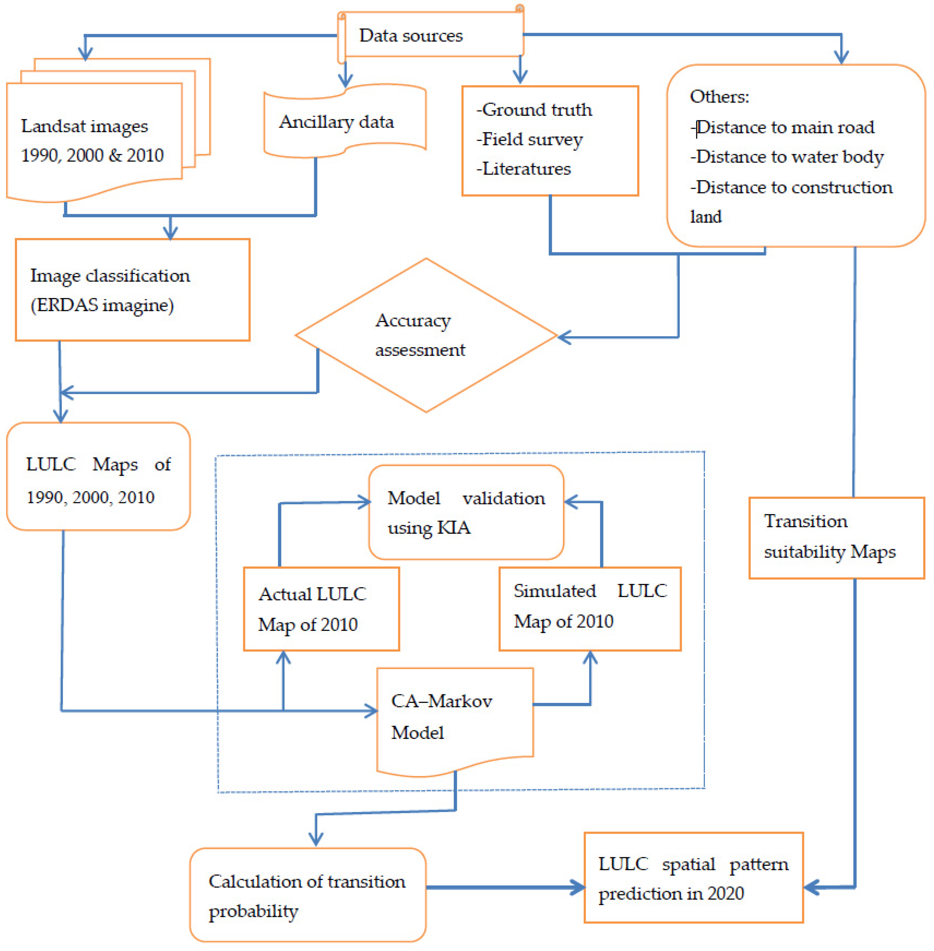
In this research, for the purpose of monitoring the current LULC management practices and assessing the effects of LULC on ESVs in the future, we focus on the forecasting of future LULC changes. This can be explored using a CA–Markov model. It has been widely cited that the CA–Markov model is the most effective method for modeling the probability of spatiotemporal change in LULC along with a geographic information system [32,33]. In the CA–Markov model, a Markov chain concerned with the temporal change occurring among the different LULC types is constructed, grounded in the probability of change matrices [34]. A CA model is used to forecast the patterns of spatial changes over time by considering the neighborhood configuration and a transition map of the LULC to be considered [35]. With the advantage of hybridizing these two methods, the CA–Markov model can achieve better simulation of LULC disparities in both space and quantity [36,37]. This feature makes the model a robust LULC change simulation [34,35].

Since the economic reform and the open door policy in the late 1970’s, the regional economic developments of China have shown incredible change [38]. As a result, primarily, many coastal areas of the country have experienced dramatic economic and spatial restructuring, resulting in tremendous LULC change [39,40,41]. Empirical investigations of the coastal areas of China have shown that changes in LULC over the past two decades have been arguably the most widespread in the country’s history [42], and the process has been more intense than in other areas and continues to worsen [43]. These impacts lead to continuous deterioration and losses in the ecological values of these fragile environments.

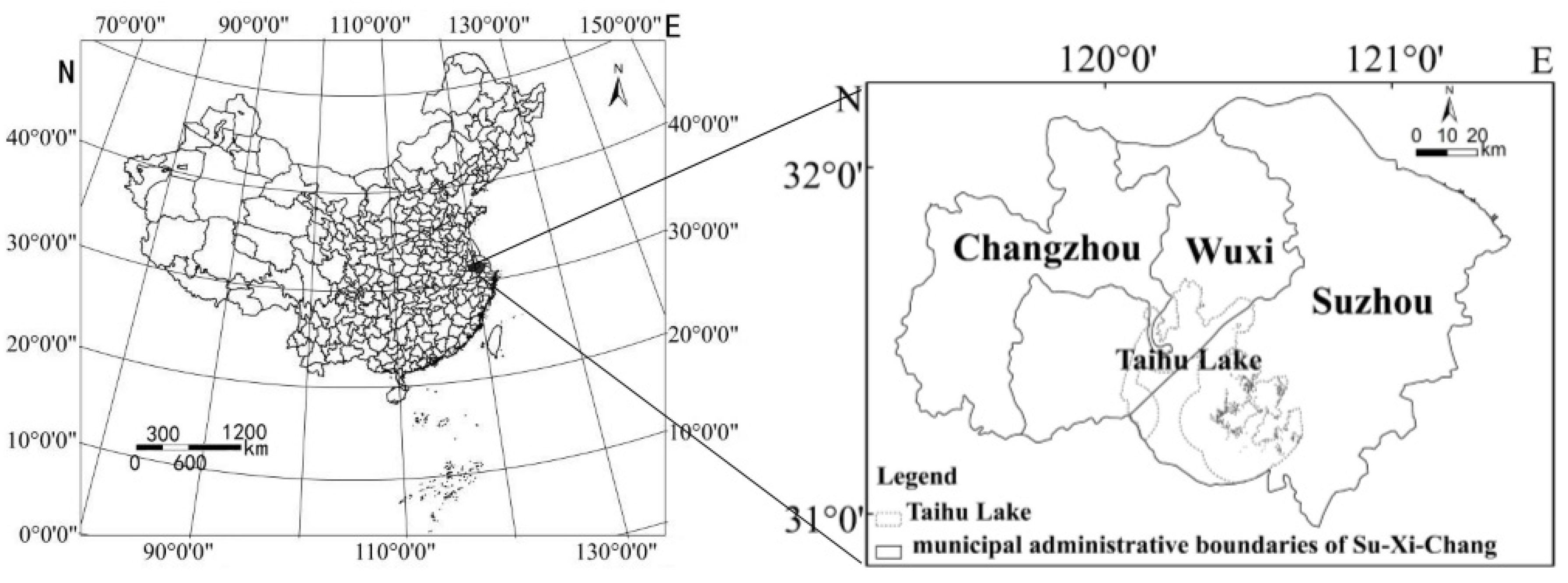
As one of the main coastal areas of China, the characteristics of LULC change in the Su-Xi-Chang region are typical and representative of those resulting from rapid population and economic growth. Because of these changes, severe LULC change and loss of the semi-natural environment and associated ESVs have been experienced in this region [44]. In their study, the authors of [41,42] indicated that there is a gap in detecting the future LULC changes and the associated threat to the ESVs of the Su-Xi-Chang region. Hence, it is important to conduct research to identify the extent and rate of LULC change for the future and to detect the impacts on ESs to sustain the ecological values of the region. Considering these factors, this study is designed with the objectives of (1) simulating and modeling the future distribution of LULC types in the Su-Xi-Chang region based on a CA–Markov model and exploring the change process; and (2) predicting the rate and extent of changes in the ESVs of the region for a future date, 2020, to enable the anticipation of future planning policies that seek to preserve the unique natural characteristics and ecological values of the studied landscape.

2. Materials and Methods

2.1. The Study Area

The Su-Xi-Chang region encompasses three municipal cities, Suzhou, Wuxi, and Changzhou. The region is in the Jiangsu Province (36°46’–32°04’N, 119°08’–121°15’E), covering a total area of 1.7 × 10⁴ km² with an average elevation below 50 meters (Figure 1). The area has a monsoon climate with a mean annual temperature and precipitation of 15.3 °C and 1092 mm, respectively.

This region reached a total population of 14.5 million (838/km²) in 2014, exceeding six times the country’s total population per km² (135.5/km²) at the same time. Similarly, during this period, the GDP per capita of China was one-third of the GDP per capita (123,325 CNY) of the Su-Xi-Chang region [45]. However, as evidenced by [44], the growth in population and economic activities led to rapid urbanization with a subsequent expansion of construction land, causing intensive LULC changes in the region.

The authors of [43] note that, because of changes in LULC, the Su-Xi-Chang region has been threatened with many environmental problems, such as the conflict over land resources and the demand for development versus the vulnerability of the coastal zone. Moreover, the authors of [31] noted that because of the loss and neglect of the environment, the consequences of uncontrolled rural industrialization in the region are particularly serious. Similarly, the authors of [41] reported that changes in LULC have influenced the environmental values of the region and suggested that a compromise should be reached between the two. Therefore, in this case, it is necessary to conduct a complete study assessing and simulating future LULC changes and predicting the ESV dynamics of the region to realize the sustainable use of land resources and ecological protection.

2.2. Data Acquisition and Processing

Landsat TM (Thematic Mapper) imagery with a 30-m spatial resolution for the years 1990, 2000, and 2010 was used as the data source for this study. Dataset selection was fixed to the summer season, when a clear sky period occurs. During which the lowest possible monthly cloud cover is achieved to minimize the cloud effect and associated reflectance. Considering these we used TM images obtained in Jun 10, July 23, and Jun 19 of 1990, 2000, and 2010 respectively. As ancillary data sources, we used topographic maps with scale of 1:100,000 and the LULC digital maps for 1990, 2000, and 2010 obtained from Institute of Geographic Sciences and Natural Resources Research, Chinese Academy of Science. Prior to interpretation, atmospheric correction and geometric rectification were performed. The topographic maps were first geo-referenced in the UTM Zone 50 projection in the Adindan datum and then projected into UTM Zone 50 with the WGS84 datum to match to the datum of the satellite image. For endmember establishment, and image classification, we used field investigations, Google Earth services, and Landsat false color imagery. A pixel-based supervised image classification with the maximum likelihood classification algorithm was used to classify the LULC classes [46,47]. It involves the prior knowledge of the area to set training sites and use of spectral information contained in individual pixels to generate the LULC classes.

Based on the features of LULC change in the studied landscape, the National Resources and Environmental Background Dynamics Remote Sensing Survey database classification system was followed to classify the LULC changes [45]. Accordingly, we classified the LULC categories of the study area into farmland, woodland, grassland, water body, wetland, and construction land for the three periods. The LULC classes used and their descriptions are presented in

Table 1. The Land Use/Land Cover (LULC) classes used and their descriptions.

LULC Classes	General Description
Farmland	Arable land, permanent crops, and heterogeneous agricultural areas
Woodland	Shrubs and semi natural vegetation transitional woodland/shrub lands, urban green areas
Grassland	Natural grasslands, pasture areas, sparsely vegetated areas
Water bodies	Permanent open water, lakes, ponds and reservoirs, coastal lagoons
Wetland	Inland wetlands and coastal wetlands
Construction land	All residential, commercial and industrial areas, continuous and non-continuous urban and rural fabrics, transportation infrastructures, mineral extraction sites

. The classified images were vectorized by exporting them from the ERDAS Imagine 9.1 image analysis software to ArcMap 10.3. Based on the computation results, the LULC changes between the studied periods were quantified to compare changes between the study periods. Furthermore, the transition probability matrixes of each LULC types were computed to show the net change and net change to persistence ratio of a given LULC type. The accuracy assessments were performed for classified images by using a minimum of 30 random points generated per class using stratified random sampling, for which, the corresponding reference classes of each LULC categories was collected from field visits, topographic maps, Google earth services, and their digital maps. After comparing the classified images with the aforementioned references, the final result of the accuracy assessment of the classified images showed precisions of 89.5%, 90.1%, and 91.0% for the years 1990, 2000, and 2010, respectively.

2.3. Determination of the Ecosystem Services Coefficients

In this study, to determine the ES coefficients of the studied landscape based on the major services it has been providing, we classified the ESs into the following nine services types, based on the works of Costanza et al. [18] and Xie et al. [48]: gas regulation, biodiversity protection, climate regulation, food production, water supply, raw materials, soil formation and protection, waste treatment, and recreation and culture. Next, the equivalent weight factors of the ESs provided by each LULC type were localized by relating them with the equivalent weight factors per hectare of the terrestrial ecosystems for China developed by Xie et al. Using the parameters set by Costanza et al., Xie et al. developed the value coefficients for Chinese ecosystems by extracting the equivalent weight factors of ESs per hectare for China’s terrestrial ecosystems [48]. This equivalent weight factor is applicable to different regions across the country by localizing the average natural food production [49]. An equivalent weight factor (the potential of an ecosystem to provide an ES) is equal to the economic value of average grain production of crop land per hectare per year. As considered by the authors of [48], generally in China, the natural food production is proposed to be 1/7 of the actual food production. In our study area, the average actual food production was 6765.33 kg ha⁻¹ from 2000 to 2010, and the average price for grain was 1.86 CNY kg⁻¹ in 2010 [34]. Thus, the computation of this value [1/7(6765.33 × 1.86)] gives us 1797.65 CNY ha⁻¹ of ESV for the equivalent weight factor for the Su-Xi-Chang region. Using this factor, the ES coefficients for each of the LULC categories of the studied landscape were computed, and the values are enumerated in

Table 2. Ecosystem Service (ES) Coefficients for each LULC type in the Su-Xi-Chang region (CNY ha⁻¹ year⁻¹).

LULC Types	Farmland	Woodland	Grassland	Water Body	Wetland	Construction Land
Coefficient	12,421.4	39,277.2	13,014.6	82,706.8	141,826.3	755.1

.

To obtain the ESV per unit area for each LULC type, each type was compared to the nearest equivalent ecosystem, as suggested by the authors of [38]. For instance, woodland equates to forestland, and construction land equates to barren land. Although the biomes used as proxies for the LULC types are clearly not perfect matches in every case, they are closely related [6].

2.4. Methods

2.4.1. LULC Change Modeling

A coupled CA–Markov model is employed to conduct LULC change modeling in this study. The CA–Markov model combination represents an advancement in spatiotemporal dynamic modeling and forecasting, achieving a better simulation of LULC changes both in quantity and space [32,37]. The algorithms in the IDRISI Andes package integrate the functions of the CA filter and Markov process, using conversion tables and conditional probabilities from the conversion map applied to simulate and forecast the states of LULC change. Therefore, to simulate future LULC changes for our study site using a CA–Markov model, the following specific processes were followed:

(1) After converting the vector data to raster, the classified LULC maps for the years 1990, 2000, and 2010 were used to obtain the transition matrices for the LULC categories between 1990 and 2000 as well as 2000 and 2010 based on the first-order Markov model [50,51].

(2) The transition suitability maps, which were used to predict the LULC in 2010 and to simulate the distribution in 2020 were generated based on the main transitions that occurred among the LULC categories from 2000 to 2010, earlier studies [42,44], field investigations, and the knowledge of the authors about the studied landscape to define the transition rules and identify factors and constraints. In addition, to determine CA filters, the regular 5 × 5 contiguity filter was used as the neighborhood definition.

(3) Based on the CA–Markov model approach, the LULC for the year 2010 was modeled using the transition probabilities from 1990 to 2000 with the LULC base map from the year 2000. Kappa statistics was used to assess the accuracy of the forecasted 2010 LULC map to evaluate its agreement with the actual 2010 LULC map (

Table 3. Markov chain transition probability matrix of LULC types for the period 2000–2010.

Land Use Types	Farmland	Woodland	Grassland	Water Body	Wetland	Construction Land
Farmland	0.7500	0.0010	0.0045	0.0140	0.0005	0.2300
Woodland	0.0030	0.9510	0.0200	0.0000	0.0050	0.0210
Grassland	0.0380	0.039	0.9121	0.0121	0.0072	0.0316
Water body	0.0000	0.001	0.0030	0.8905	0.0202	0.0900
Wetland	0.0078	0.0000	0.0200	0.04	0.8835	0.0432
Construction land	0.0000	0.0140	0.0000	0.0004	0.0000	0.9856

).

(4) Finally, following the same process, the LULC for the year 2020 was projected with the CA–Markov model in IDRISI using the transition probabilities from 2000 to 2010 and the LULC base map from the year 2010. Figure 2 shows a schematic of the technical method followed in the CA-Markov LULC change model.

2.4.2. Prediction of ESV Change

In this study, the prediction of changes in ESVs involved the use of the projected area of each of the LULC types and the modified ES coefficients of the corresponding biomes of the six LULC types considered (under Section 2.2). Furthermore, the ESVs for the past two decades were also assessed to compare changes in values with the future. After determining the ESV per unit area for each LULC type, the service values of each LULC category, their corresponding service function and the total ESVs for both periods (past and future) were obtained using the following Equations [49]:

$$ES{V}_k=A_k\times V{C}_k$$

(1)

$$ES{V}_f={\displaystyle \sum }_k{A}_k\times V{C}_{kf}$$

(2)

$$ESVt={\displaystyle \sum }_k{A}_k\times V{C}_k$$

(3)

where ESV_k, ESV_f, and ESV_t denote the ESV for LULC type k, service function f, and the total ESV, respectively; A_k is the area (ha) for LULC type k; VC_k is the value coefficient (yuan ha⁻¹ year⁻¹) for LULC type k; and VC_kf is the value coefficient (yuan ha⁻¹ year⁻¹) for LULC type k with ES function type f.

Since the biomes we used as proxies for LULC categories are not perfect matches (as revealed above, Section 2.3), and since uncertainties exist in the value coefficients, an additional sensitivity analysis was needed to determine the percentage change in the ESV for a given percentage change in the value coefficient. In each analysis, the coefficient of sensitivity (CS) was calculated using the standard economic concept of elasticity, i.e., the percentage change in the output for a given percentage change in an input [6,52,53] as follows:

$$CS=\frac{\left(ES{V}_j-ES{V}_i\right)/ES{V}_i}{\left(V{C}_{jk}-V{C}_{ik}\right)/V{C}_{ik}}$$

(4)

where ESV is the estimated ecosystem service value, VC is the value coefficient, i and j represent the initial and adjusted values, respectively, and k represents the LULC category. If CS > 1, then the estimated ecosystem value is elastic with respect to that coefficient, and it is important to accurately define VC, but if CS < 1, then the estimated ecosystem value is considered to be inelastic, and the results of the ESV calculations will be reliable even if the VC value has a relatively low accuracy.

3. Results and Discussion

3.1. LULC Change Modeling

3.1.1. Analysis of Transition Probability Matrix

The LULC transfer directions for the study area from one type to another that have been calculated using the Markov model are shown in the transition probability matrix (Table 3). The bolded values along the transition probability diagonal indicate the probability of a LULC type remaining unchanged from time t₀ to time t (t > t₀), whereas the cross-diagonal shows the probability that a given LULC undergoes a change from one category to another. The results show that during the study period, different LULC types exhibited various dynamic conditions. Construction land, woodland, and grassland are the most stable LULC types, with transition probabilities exceeding 0.91. Farmland, wetland, and water body show less persistence, with probabilities of 0.75, 0.88, and 0.89, respectively (Table 3).

The early 21st century, between 2000 and 2010, was a time when the second round of rapid growth of industrialization and urbanization occurred in China [54], in particular in the Su-Xi-Chang region [42,44]. This process resulted in less stability of various LULC types in the region. During this period, the expansion of construction land consumed large quantities of farmland, water body, and wetland land cover (Table 3). In addition to the expansion in construction land, profit-oriented farming practices involving the conversion of farmland to fishponds [44] were another reason that farmland was the most dynamic with lowest transition persistence (0.75) relative to other LULC types. However, construction land has the highest transition persistence (0.99). This could be because, as a policy, the government identified the Su-Xi-Chang region as place to build new countryside developments, and as an industrial zone, because of its location in a coastal area [42]. In addition, our results indicate that, during this period, in order to meet the high demand for construction land expansion in addition to farmland, huge areas of wetlands as well as water bodies with high environmental values were extensively utilized (Table 3).

3.1.2. Prediction of LULC Changes Based on the CA–Markov Model

A comparison of the actual LULC map for the year 2010 with the CA–Markov-simulated map, based on the Kappa statistic (

Table 4. Assessment of the agreement between the predicted and actual LULC in 2010.

Accuracy Values	Farmland	Woodland	Grassland	Water Body	Wetland	Construction Land
User’s accuracy	97.17	98.23	100	97.25	98.17	97.82
Producer’s accuracy	92.89	95.75	97.54	95.78	100	89.12
Overall accuracy	91.31
Overall Kappa	0.91

), as well as a comparison of each area of the simulated LULC types with the actual area (Figure 3), were used for model validation. The Kappa statistics values (0.91) and an overall accuracy exceeding 91% (Table 4) show that there is good agreement between the predicted result and the actual value of the LULC types for the base year. As shown in Figure 3, the change in magnitude between the two maps of the year 2010 reveals that all LULC classes have relative errors of less than 5%. Furthermore, a visual interpretation of the simulated and actual maps for the year 2010 (Figure 4c,d) demonstrates that there is an obvious similarity between the two. As it has been also considered by earlier studies in other areas [32,34,35], these results indicate that the CA–Markov model was effective in simulating LULC change in 2010. Therefore, the model can be reliable in predicting future LULC change with the assumption that an unvarying rate of change will occur in the future.

After the successful simulation of changes in 2010, the future LULC change for the year 2020 was predicted by using a land-use base map for 2010, the transition matrix for 2000 to 2010, and a potential transition map for 2010. Figure 4a–c,e show the tendency of the spatial distributions of LULC changes for the four periods 1990, 2000, 2010, and 2020, and

Table 5. LULC changes between 1990, 2000, 2010, and 2020 in the Su-Xi-Chang region.

LULC Type	Total Area Coverage (Ha)				Gain/Loss (%) Between Different Times
	1990	2000	2010	2020	1990–2000	2000–2010	2010–2020
Farmland	922,383	864,338	647,986	596,312	−6.29	−25	−8
Woodland	116,890	117,154	119,831	120,379	0.23	2.29	0.48
Grassland	1745	1592	2203	2442	−8.77	38.38	10.85
Water body	516,757	499,309	485,055	474,538	−3.38	−2.85	−2.17
Wetland	5059	3672	3454	3141	−27.42	−5.94	−9.06
Construction land	181,790	258,559	486,095	547,812	42.23	88	12.7
Total	1,744,624	1,744,624	1,744,624	1,744,624	−	−	−

reveals the magnitude of changes for the same periods. As can be observed from the spatial pattern analysis (Figure 4), a clear spatial change in LULC is observed throughout the study period. As presented in Figure 4a, in 1990, farmland and water body were the dominant LULC types, during which construction land was mainly limited to the three areas: the central part of the three main metropolitan areas of the region, Suzhou, Wuxi, and Changzhou. In the next decade, construction land began to expand around the previously existing areas and spread to other parts of the region (Figure 4b). In the following period (2010), during which the second round of rapid development of urbanization and industrialization arose in the region [31,33], construction land expanded and increased by 88% of its total area in the preceding decade (Figure 4c and Table 5), mainly at the expense of farmland, wetland and water body cover types (Table 3). Furthermore, as indicated in the predicted result (Figure 4e), the spatial pattern of construction land continues to expand and is projected to cover more than 31% of the total study area in 2020 (Table 5).

From the temporal pattern analysis (Table 5), the general tendencies of the changes in LULC during the course of the study show that in 1990, farmland, water body, construction land, and woodland were the major LULC classes, accounting for 52.87%, 29.62%, 10.42%, and 6.7% of the total landscape, respectively. This order continued sequentially up to the second decade, 2010, with various rates of change (gain/loss). However, in 2020, the predicted results show that with a more than three-fold increase over its base year area and covering greater than 31% of the total study area, construction land will become the dominant LULC next to farmland (34%), and water body is the third largest (27.2%), followed by woodland (6.9%).

In the period between 1990 and 2000, farmland, water body, and construction land exhibited changes of −6.3%, −3.4%, and +42.2% in their total area, respectively. The same trends of change were observed for these three LULC cover types in the period from 2010 to 2020 with different rates of change per annum. Farmland continued to decrease by −0.8% per year, water body decreases by −0.2%, while construction land increases by about one-seventh of the growth it had been showing in the former decade (Table 5).

Over the period 1990 to 2000, the wetland and grassland cover types showed a reduction of −27.4% and −8.8% in their total areas, respectively. Between 2000 and 2010, grassland showed an annual rate of increase of 3.8%, while wetland continued to decrease with a rate of −0.6% per annum. The same trend continues from 2010 to 2020 for both LULC types, in which wetland decreases with an annual rate of −0.9% and grassland increases by 1.1%, as compared to the earlier decade. Both woodland and construction land exhibit an increasing trend to varying degrees throughout the study period (Table 5). Despite the fact that construction land continues to increase with a higher rate than other LULC categories, our results indicate that the rate of expansion it had shown between 2000 and 2010 was the largest in the study period. This result may be because this period was concurrent with the second round of rapid growth of industrialization and urbanization that occurred in the region [42,44], in which large quantities of undeveloped areas (non-construction land) were converted to developed areas (construction land). Specifically, this conversion was of agricultural land, wetland and water bodies with high environmental values into construction land with low environmental value.

The general trend of LULC changes in the region reveal that the changes experienced in the recent past are likely to continue in the future (2020). Even though their rates of change (gains/losses) are comparably less than in the former periods, the predicted LULC change shows that the farmland, water body, and wetland categories will continue to decrease (Table 5). These LULC types have been largely replaced by construction land, as shown (Table 3). Thus, the ongoing trends of change have placed pressure on LULC classes with significant environmental values, which could result in losses in the semi-natural environment of the region. As considered by [42], this could have an adverse effect on the environmental sustainability of the area unless a proper land use plan with emphasis on controlling construction land (industrial, commercial, residential) encroachment on farmland, wetland, and water bodies is achieved.

3.2. Ecosystem Services Value Prediction

3.2.1. Predicted ESVs and Trends in ESV Change for Each LULC Type

The predicted ESVs for each LULC category and the total value for the year 2020 were computed using the modified ES coefficients for the corresponding biome (Table 2) and the projected area of each LULC type (Table 5). Similarly, to compare changes in the ESVs over the past two decades with the predicted values, the ESVs of each LULC type and the total value for each study year (1990, 2000, and 2010) were obtained using modified ES coefficients and the area covered by each LULC type during these periods (

Table 6. Total Ecosystem Service Value (ESV) for each land use type in the Su-Xi-Chang region in 1990, 2000, 2010, and 2020.

LULC Type	ESV (×109 CNY yr−1 )
	1990	%	2000	%	2010	%	2020	%	Over All Change
									1990–2020	%
FL	11.4573	19.2	10.7363	18.78	8.0489	14.97	7.407	14.16	−326,071	–35.35
WOL	4.5911	7.69	4.6015	8.05	4.7066	8.75	4.7282	9.04	3489	2.98
GL	0.0227	0.04	0.0207	0.04	0.0287	0.053	0.0318	0.06	697	39.94
WB	42.7393	71.63	41.2962	72.22	40.1173	74.62	39.2475	75.08	−42,219	−8.17
WL	0.7175	1.2	0.5208	0.91	0.4899	0.91	0.4455	0.85	−1918	−37.91
CL	0.1373	0.23	0.1952	0.34	0.3671	0.68	0.4137	0.79	366,022	201.34
Total	59.6652	100	57.1775	100	53.7585	100	52.2737	100	−	−

where: FL–Farmland, WOL–Woodland, GL–Grassland, WB–Water body, WL–Wetland, CL–Construction land.

). The calculated ES coefficients for each of the classes are described in Table 2.

The results show that each LULC type exhibited different ESVs as well as various gain/loss trends throughout the course of the study (Table 6 and Figure 5). For instance, as shown in Table 6, the ESV of farmland continued to decrease steadily throughout the study period and showed a total loss of more than 35% compared to the base year value. Even though the Su-Xi-Chang region is known as a primary grain production area along the east coastal zone of China [42], the current LULC change, particularly the conversion of farmland with high ES functions, into construction land with low ES functions (Table 3) has led to a reduction in the ES provisioning of the region. Similarly, the ESV of water bodies shows a decreasing tendency. In addition to having a high ES coefficient close to that of wetland (Table 2), the water body cover type has the highest proportion of total area next to farmland (Table 5), resulting in this cover type having the highest ESV of all LULC types (Table 6). However, continuous extraction and utilization of water bodies for various purposes in the region have caused a decrease in the area of water body coverage, consequently reducing its ES provisioning. Currently, its ESV has been decreasing with an average rate of −0.3% per annum (Figure 5), amounting to a loss of 116.4 million CNY year⁻¹.

Wetland is the most important LULC for providing diverse ESs than any other terrestrial biome [55]. It has many potential roles, ranging from environmental protection to climate mitigation. Wetlands provide many service functions, such as sequestering releases from various polluting industries as well as residential pollution. As depicted in Table 6 and Figure 5, the ESV of wetland decreased continuously throughout the study period. Wetland has an ES coefficient more than 1.7 times greater than water body cover and approximately 11.5 times that of farmland (Table 2). However, in this region, the service provision value for wetlands is far less than farmland or water bodies. In addition to its smaller area coverage compared to other LULC classes, except for grassland (Table 5), the gradual reduction of wetland area for construction land expansion (Table 3) has caused it to provide less ESV. This shows that, as also considered by [56] in the West Songneu Plain of China, because land was becoming scarce for construction land expansion, wetland becomes the target for construction development, causing losses of environmentally viable biomes. Moreover, Figure 5 reveals that even though the increase in ESVs both woodland and grassland had shown did not offset the decreased values showed by other LULC categories, their ESVs increased steadily throughout the study period, in which the rate for woodland was higher than that of grassland.

As depicted in the results, in each study period, water body and farmland are the dominant LULC categories, providing an average of more than 90% of the total ESVs throughout the study period. This could be because of their larger area as well as the relatively higher ES coefficients compared to other LULC categories. The total ESVs of the studied landscape decreased from 59.6652 × 10⁹ CNY in 1990 to 52.2737 × 10⁹ CNY in 2020, amounting to a total loss of 7.3915 billion CNY (Table 6). Compared to other findings in other areas of China [57,58,59], this loss could be very high. This result is because of the extensive expansion of construction land with a low ESV at the expense of farmland, water body and wetland coverage with higher ESVs (Table 3). The authors of [44] reported that in the recent past, the increase in construction land due to rapid urbanization and industrialization caused a deterioration of the semi-natural landscape of the Su-Xi-Chang region. Likewise, our predicted results indicate (Table 6 and Figure 5) that this trend of change (losses) in the total ESVs of the region will continue in the future, 2020, unless proper LULC management is practiced to halt and reverse the situation.

The overall trends in the ESVs of individual ecosystem functions (ESV_f) for each of the study periods and their overall changes shown in

Table 7. Values of ecosystem service functions (ESV_f) for the Su-Xi-Chang region in 1990, 2000, 2010 and 2020.

Ecosystem Service Function	1990		2000		2010			2020
	ESVf (×109 CNY yr−1)	%	ESVf (×109 CNY yr−1)	%	ESVf (×109 CNY yr−1)		%	ESVf (×109 CNY yr−1)	%
Gas regulation	1.7305	2.9	1.635	2.85	1.4512		2.7	1.3984	2.67
Climate regulation	2.628	4.41	2.4798	4.32	2.1288		3.96	2.0311	3.88
Water supply	20.7703	34.82	20.0347	34.93	19.3011		35.9	18.8578	36.07
Soil formation and retention	3.2778	5.49	3.1169	5.43	2.5852	4.81		2.4554	4.69
Waste treatment	20.0734	33.64	19.2878	33.63	18.1885	33.83		17.6846	33.83
Biodiversity protection	4.3125	7.23	4.202	7.32	4.0172	7.47		3.9442	7.54
Food	1.7789	2.98	1.6722	2.92	1.2854	2.39		1.1918	2.28
Raw material	0.7223	1.21	0.7125	1.24	0.6859	1.28		0.679	1.29
Recreational and culture	4.3709	7.32	4.2219	7.36	4.1151	7.66		4.0312	7.71
Total	59.6652	100	57.3709	100	53.7584	100		52.2736	100

. Water supply, waste treatment, recreational and cultural functions, and biodiversity protection are among the dominant ecosystem service functions provided by the ESs of the region, accounting for 84% of the total value during the study periods and amounting to 50.12 billion CNY, 48.19 billion CNY, 45.12 billion CNY and 43.9 billion CNY monetary values in 1990, 2000, 2010, and 2020, respectively. Of these service functions, the water supply services category has the largest share, followed by waste treatment services.

3.2.2. Ecosystem Services Sensitivity Analyses

Using Equation (4), the percentage change in the estimated total ESVs and the corresponding coefficient of sensitivity (CS) resulting from a 50% adjustment in the value of the ESV coefficients for selected LULC classes were computed (

Table 8. Estimated total ESV (×10⁹ CNY/year) in the Su-Xi-Chang region after adjusting the ecosystem services valuation coefficients (VC) and the coefficient of sensitivity (CS) associated with these adjustments.

Change in Value Coefficient	ESV		1990–2020 Change		Effect of Changing CV from Original Value
					1990		2020
	1990	2020	CNY	%	%	CS	%	CS
Farmland VC +50%	65.3938	55.9772	−9.4166	−14.4	±9.60	±0.19	±7.08	±0.14
Farmland VC −50%	53.9365	48.5702	−5.3663	−9.95
Woodland VC +50%	61.9608	54.4477	−7.5131	−12.13	±3.85	±0.08	±4.16	±0.08
Woodland VC −50%	57.3697	49.9096	−7.4601	−13
Water body VC +50%	81.0349	71.8975	−9.1374	−11.28	±35.82	±0.71	±37.54	±0.75
Water body VC −50%	38.2956	32.65	−5.6456	−14.74
Wetland VC +50%	60.0239	52.4964	−7.5275	−12.54	±0.60	±0.01	±0.43	±0.01
Wetland VC −50%	59.3064	52.0509	−7.2555	−12.23

). As discussed in Section 2.4.2, a reasonably low sensitivity of ESVs to changes in the ES coefficients (i.e., CS < 1) should be attained for the results of our analysis to be reliable. In all cases, the computed CS results were less than one, indicating that the total ESVs estimated in this study was relatively inelastic with respect to changes in the ESV coefficient (Table 8). The highest coefficient of sensitivity was registered for the water body class (0.71 to 0.75) because of the large area cover and high value of coefficient for this LULC type. By calculating the ESVs for 1990 and 2020 and analyzing changes over this time period, errors and uncertainties could be reduced or offset. On the whole, the computed sensitivity analysis indicated that the values of VC for the study area are reliable regardless of uncertainties in the ESV coefficients.

4. Conclusions

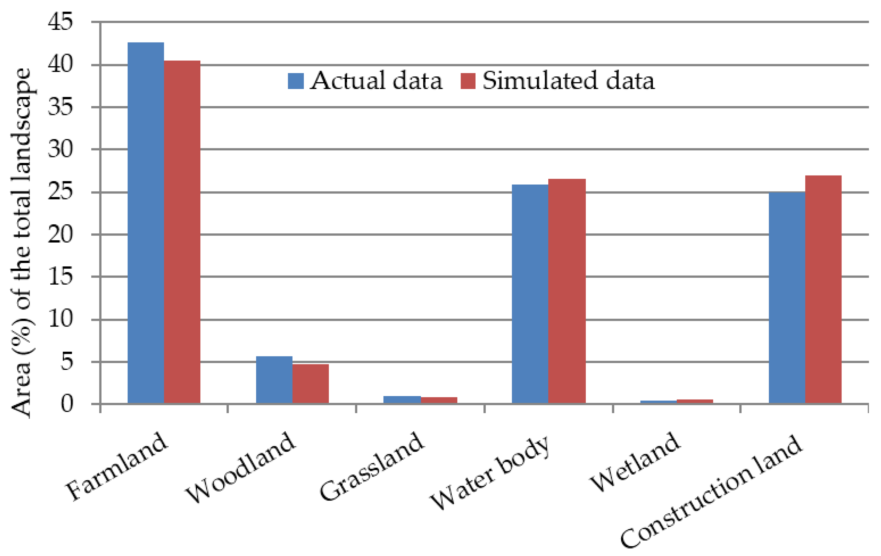
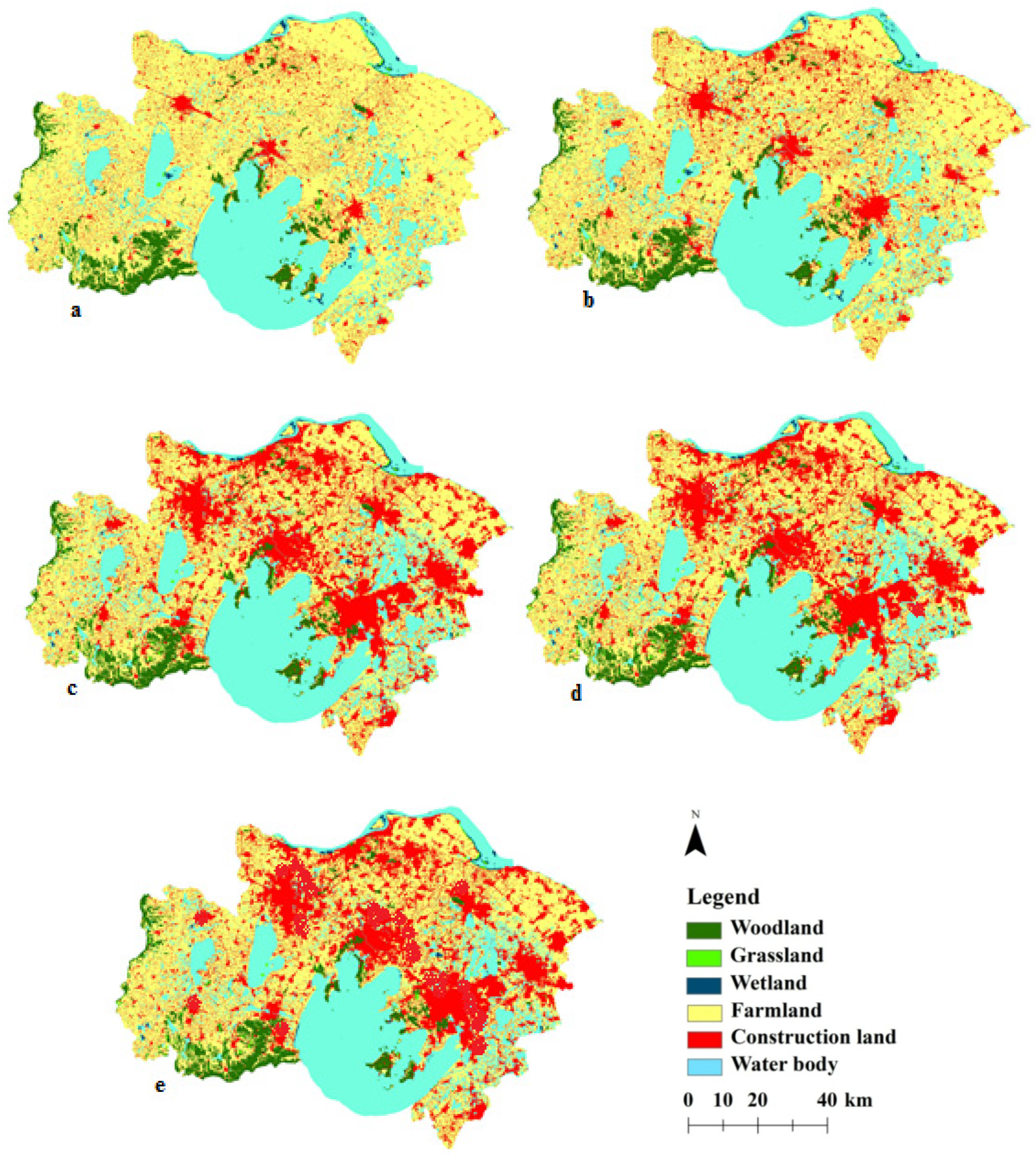
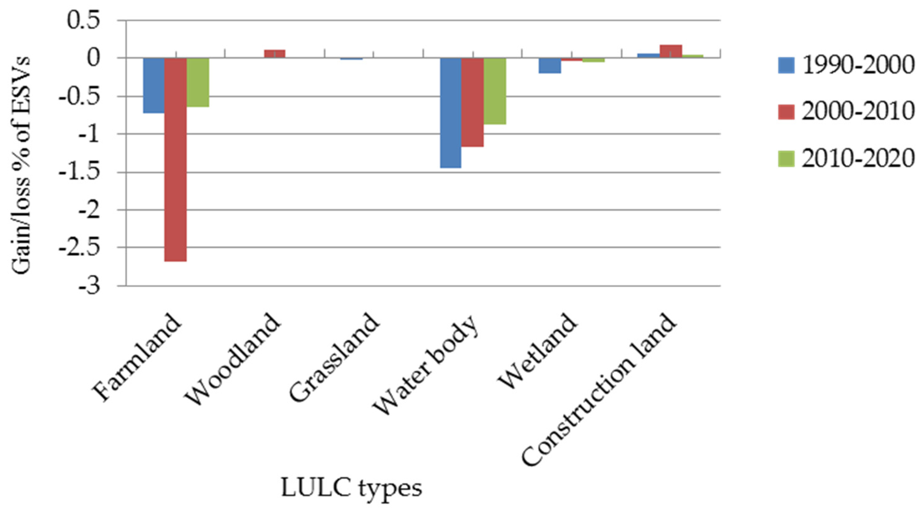
This study explored a future LULC change simulation using a CA–Markov model in combination with GIS technology and predicted the subsequent changes in ESV by using land use data and the modified ES coefficients of the studied landscape. The validation of our model with the actual data of the base year (2010) shows an overall satisfactory result, revealing that CA–Markov is an appropriate model for predicting future LULC change. The results of the predicted future LULC area changes indicate decreases in farmland, wetland, and water bodies, but increases in construction land, woodland, and grassland. From the temporal patterns of the changes between 2010 and 2020, wetland decreases at a higher rate, followed by farmland and water bodies. Furthermore, the patterns of LULC change over the three decades show that wetland decreased at an average rate of 14%, followed by farmland (13%) and water bodies (2.8%). However, at the expense of these LULC categories, construction land is expanding at a higher average rate (48%) than other LULC types. As a consequence, with the current trend in land management, these three LULC types with high ecological values have been continuously declining, leading to losses in the environmental and ecological values of the region.

The predicted ESV results reveal that each LULC category exhibited different trends of changes, in which the values for farmland, wetland, and water bodies were reduced, whereas the values for woodland, grassland, and construction land showed an increase. In 2020, farmland and water body are the dominant LULC types, providing more than 90% of the total ESV. Over the study period, the total ESV of the Su-Xi-Chang region decreased from 59.6652 billion CNY in 1990 to 52.2737 billion CNY in 2020, mainly because of the loss of farmland, water bodies, and wetland. During the study period, the water body class produced the largest proportion of the total ESV (73%), and combining water body and farmland accounted for more than 90% of the total ESV, indicating that the two LULC categories play a role in providing the highest ESs in the region.

Water supply and waste treatment were the top two ecological functions, accounting for more than 68% of the total, mainly provided by water body and wetland cover types, followed by woodland and farmland. Even though water body and farmland are the dominant LULC classes providing a major share of the ESVs in the Su-Xi-Chang region, these two categories are becoming highly degraded. For sustainable management, a compromise between the current patterns of LULC change and ecological protection must be reached. A reasonable land use plan should be made with an emphasis on controlling construction land (industrial, commercial, residential) encroachment on farmland, wetlands, and water bodies. Furthermore, the rules of ecological protection should be followed in LULC management to preserve ecological resources and benefit society. Thus, decision makers should plan alternative conservation activities to enact improved LULC management practices for sustainable and balanced ecological protection.

References

1. Guan, D.J.; Li, H.F.; Inohae, T.; Su, W.C.; Nagaie, T.; Hokao, K. Modeling urban land use change by the integration of cellular automaton and Markov model. Ecol. Model. 2011, 222, 3761–3772. [Google Scholar] [CrossRef]
2. Halmy, M.W.A.; Gessler, P.E.; Hicke, J.A.; Salem, B.B. Land use/land cover change detection and prediction in the north-western coastal desert of Egypt using Markov-CA. Appl. Geogr. 2015, 63, 101–112. [Google Scholar] [CrossRef]
3. Zheng, H.W.; Shen, G.Q.; Wang, H.; Hong, J.K. Simulating land use change in urban renewal areas: A case study in Hong Kong. Habitat Int. 2015, 46, 23–34. [Google Scholar] [CrossRef]
4. Garedew, E.; Sandewall, M.; Söderberg, U.; Campbell, B.M. Land-use and land-cover dynamics in the central rift valley of Ethiopia. Environ. Manag. 2009, 44, 683–694. [Google Scholar] [CrossRef] [PubMed]
5. Kindu, M.; Schneider, T.; Teketay, D.; Knoke, T. Drivers of land use/land cover changes in Munessa-Shashemene landscape of the south-central highlands of Ethiopia. Environ. Monit. Assess. 2015, 187, 452. [Google Scholar] [CrossRef] [PubMed]
6. Kreuter, U.P.; Harris, H.G.; Matlock, M.D.; Lacey, R.E. Change in ecosystem service values in the San Antonio area, Texas. Ecol. Econ. 2001, 39, 333–346. [Google Scholar] [CrossRef]
7. Li, R.-Q.; Dong, M.; Cui, J.-Y.; Zhang, L.-L.; Cui, Q.-G.; He, W.-M. Quantification of the impact of land-use changes on ecosystem services: A case study in Pingbian County, China. Environ. Monit. Assess. 2007, 128, 503–510. [Google Scholar] [CrossRef] [PubMed]
8. Peng, J.; Wang, Y.L.; Wu, J.S.; Yue, J.; Zhang, Y.A.; Li, W.F. Ecological effects associated with land-use change in China’s southwest agricultural landscape. Int. J. Sust. Dev. World Ecol. 2006, 13, 315–325. [Google Scholar] [CrossRef]
9. Zhao, B.; Kreuter, U.; Li, B.; Ma, Z.; Chen, J.; Nakagoshi, N. An ecosystem service value assessment of land-use change on Chongming Island, China. Land Use Policy 2004, 21, 139–148. [Google Scholar] [CrossRef]
10. Portela, R.; Rademacher, I. A dynamic model of patterns of deforestation and their effect on the ability of the Brazilian Amazonia to provide ecosystem services. Ecol. Model. 2001, 143, 115–146. [Google Scholar] [CrossRef]
11. Temesgen, H.; Nyssen, J.; Zenebe, A.; Haregeweyn, N.; Kindu, M.; Lemenih, M.; Haile, M. Ecological succession and land use changes in a lake retreat area (Main Ethiopian Rift Valley). J. Arid Environ. 2013, 91, 53–60. [Google Scholar] [CrossRef]
12. Wang, S.; Wu, B.; Yang, P. Assessing the changes in land use and ecosystem services in an oasis agricultural region of Yanqi Basin, Northwest China. Environ. Monit. Assess. 2014, 186, 8343–8357. [Google Scholar] [CrossRef] [PubMed]
13. Szumacher, I.; Pabjanek, P. Temporal Changes in Ecosystem Services in European Cities in the Continental Biogeographical Region in the Period from 1990–2012. Sustainability 2017, 9, 665. [Google Scholar] [CrossRef]
14. Kindu, M.; Schneider, T.; Teketay, D.; Knoke, T. Changes of ecosystem service values in response to land use/land cover dynamics in Munessa–Shashemene landscape of the Ethiopian highlands. Sci. Total Environ. 2016, 547, 137–147. [Google Scholar] [CrossRef] [PubMed]
15. Bateman, I.J.; Harwood, A.R.; Mace, G.M.; Watson, R.T.; Abson, D.J.; Andrews, B.; Binner, A.; Crowe, A.; Day, B.H.; Dugdale, S. Bringing ecosystem services into economic decision-making: Land use in the United Kingdom. Science 2013, 341, 45–50. [Google Scholar] [CrossRef] [PubMed]
16. Birkhofer, K.; Diehl, E.; Andersson, J.; Ekroos, J.; Früh-Müller, A.; Machnikowski, F.; Mader, V.L.; Nilsson, L.; Sasaki, K.; Rundlöf, M. Ecosystem services—current challenges and opportunities for ecological research. Front. Ecol. Evol. 2015, 2, 87. [Google Scholar] [CrossRef]
17. Wei, H.; Fan, W.; Ding, Z.; Weng, B.; Xing, K.; Wang, X.; Lu, N.; Ulgiati, S.; Dong, X. Ecosystem Services and Ecological Restoration in the Northern Shaanxi Loess Plateau, China, in Relation to Climate Fluctuation and Investments in Natural Capital. Sustainability 2017, 9, 199. [Google Scholar] [CrossRef]
18. Costanza, R.; dArge, R.; deGroot, R.; Farber, S.; Grasso, M.; Hannon, B.; Limburg, K.; Naeem, S.; ONeill, R.V.; Paruelo, J.; et al. The value of the world's ecosystem services and natural capital. Nature 1997, 387, 253–260. [Google Scholar] [CrossRef]
19. Schnegg, M.; Rieprich, R.; Pröpper, M. Culture, nature, and the valuation of ecosystem services in Northern Namibia. Ecol. Soc. 2014, 19, 26. [Google Scholar] [CrossRef]
20. Fu, Q.; Li, B.; Yang, L.; Wu, Z.; Zhang, X. Ecosystem Services Evaluation and Its Spatial Characteristics in Central Asia’s Arid Regions: A Case Study in Altay Prefecture, China. Sustainability 2015, 7, 8335–8353. [Google Scholar] [CrossRef]
21. Zhang, Y.; Zhao, L.; Liu, J.; Liu, Y.; Li, C. The Impact of Land Cover Change on Ecosystem Service Values in Urban Agglomerations along the Coast of the Bohai Rim, China. Sustainability 2015, 7, 10365–10387. [Google Scholar] [CrossRef]
22. Arunyawat, S.; Shrestha, R.P. Assessing Land Use Change and Its Impact on Ecosystem Services in Northern Thailand. Sustainability 2016, 8, 768. [Google Scholar] [CrossRef]
23. Araya, Y.H.; Cabral, P. Analysis and modeling of urban land cover change in Setúbal and Sesimbra, Portugal. Remote Sens. 2010, 2, 1549–1563. [Google Scholar] [CrossRef]
24. Jat, M.K.; Garg, P.K.; Khare, D. Monitoring and modelling of urban sprawl using remote sensing and GIS techniques. Int. J. Appl. Earth Obs. 2008, 10, 26–43. [Google Scholar] [CrossRef]
25. Fischer, G.; Sun, L.X. Model based analysis of future land-use development in China. Agric. Ecosyst. Environ. 2001, 85, 163–176. [Google Scholar] [CrossRef]
26. Han, H.; Yang, C.; Song, J. Scenario simulation and the prediction of land use and land cover change in Beijing, China. Sustainability 2015, 7, 4260–4279. [Google Scholar] [CrossRef]
27. Santé, I.; García, A.M.; Miranda, D.; Crecente, R. Cellular automata models for the simulation of real-world urban processes: A review and analysis. Landsc. Urban Plan. 2010, 96, 108–122. [Google Scholar] [CrossRef]
28. Gautam, A.P.; Webb, E.L.; Shivakoti, G.P.; Zoebisch, M.A. Land use dynamics and landscape change pattern in a mountain watershed in Nepal. Agric. Ecosyst. Environ. 2003, 99, 83–96. [Google Scholar] [CrossRef]
29. Porter-Bolland, L.; Ellis, E.A.; Gholz, H.L. Land use dynamics and landscape history in La Montana, Campeche, Mexico. Landsc. Urban Plan. 2007, 82, 198–207. [Google Scholar] [CrossRef]
30. Verburg, P.H.; Overmars, K.P.; Huigen, M.G.; de Groot, W.T.; Veldkamp, A. Analysis of the effects of land use change on protected areas in the Philippines. Appl. Geogr. 2006, 26, 153–173. [Google Scholar] [CrossRef]
31. Xie, Y.C.; Batty, M.; Zhao, K. Simulating emergent urban form using agent-based modeling: Desakota in the suzhou-wuxian region in China. Ann. Assoc. Am. Geogr. 2007, 97, 477–495. [Google Scholar] [CrossRef]
32. Sang, L.; Zhang, C.; Yang, J.; Zhu, D.; Yun, W. Simulation of land use spatial pattern of towns and villages based on CA-Markov model. Math. Comput. Model. 2011, 54, 938–943. [Google Scholar] [CrossRef]
33. Yu, F. Study on forecast of land use change based on Markov-CA. Land Res. Inf. (In Chinese) 2009, 4, 38–46. [Google Scholar]
34. Subedi, P.; Subedi, K.; Thapa, B. Application of a hybrid cellular automaton–Markov (CA-Markov) Model in land-use change prediction: A case study of saddle creek drainage Basin, Florida. Appl. Ecol. Environ. Sci. 2013, 1, 126–132. [Google Scholar] [CrossRef]
35. Kityuttachai, K.; Tripathi, N.K.; Tipdecho, T.; Shrestha, R. CA-Markov Analysis of Constrained Coastal Urban Growth Modeling: Hua Hin Seaside City, Thailand. Sustainability 2013, 5, 1480–1500. [Google Scholar] [CrossRef]
36. White, R.; Engelen, G. Cellular dynamics and GIS: Modelling spatial complexity. J. Geogr. Syst. 1994, 1, 237–253. [Google Scholar]
37. Yang, X.; Zheng, X.-Q.; Chen, R. A land use change model: Integrating landscape pattern indexes and Markov-CA. Ecol. Model. 2014, 283, 1–7. [Google Scholar] [CrossRef]
38. Wei, Y.H.D.; Fan, C.C. Regional inequality in China: A case study of Jiangsu Province. Prof. Geogr. 2000, 52, 455–469. [Google Scholar] [CrossRef]
39. Li, X.; Yeh, A.G.O. Analyzing spatial restructuring of land use patterns in a fast growing region using remote sensing and GIS. Landsc. Urban Plan. 2004, 69, 335–354. [Google Scholar] [CrossRef]
40. Long, H.L.; Hellig, G.K.; Li, X.B.; Zhang, M. Socio-economic development and land-use change: Analysis of rural housing land transition in the Transect of the Yangtse River, China. Land Use Policy 2007, 24, 141–153. [Google Scholar] [CrossRef]
41. Yirsaw, E.; Wu, W.; Temesgen, H.; Bekele, B. Effect of temporal land use/land cover changes on ecosystem services value in coastal area of China: The case of Su-Xi-Chang region. Appl. Ecol. Envion. Res. 2016, 14, 409–422. [Google Scholar] [CrossRef]
42. Liu, Y.S.; Wang, J.Y.; Long, H.L. Analysis of arable land loss and its impact on rural sustainability in Southern Jiangsu Province of China. J. Environ. Manage. 2010, 91, 646–653. [Google Scholar] [CrossRef] [PubMed]
43. Zhou, X.; Chen, L.; Xiang, W. Quantitative analysis of the built-up area expansion in Su-Xi-Chang region, China. J. Appl. Ecol. (In Chinese) 2014, 25, 1422–1430. [Google Scholar]
44. Long, H.; Liu, Y.; Wu, X.; Dong, G. Spatio-temporal dynamic patterns of farmland and rural settlements in Su–Xi–Chang region: Implications for building a new countryside in coastal China. Land Use Policy 2009, 26, 322–333. [Google Scholar] [CrossRef]
45. National Bureau of Statistics of China [NBSC] (2014): China Statistical Yearbook; China Statistics Press: Beijing, China, 2015.
46. Jensen, J.R. Remote Sensing of the Environment: An Earth Resource Perspective 2/e; Pearson Education India: Noida, India, 2009. [Google Scholar]
47. Richards, J.; Jia, X. Remote Sensing Digital Image Analysis; Springer: Berlin & Heidelberg, Germany, 1999. [Google Scholar]
48. Xie, G.-D.; Lu, C.-X.; Leng, Y.-F.; Zheng, D.; Li, S. Ecological assets valuation of the Tibetan Plateau. J. Nat. Resour. 2003, 18, 189–196. [Google Scholar]
49. Liu, Y.; Li, J.; Zhang, H. An ecosystem service valuation of land use change in Taiyuan City, China. Ecol. Model. 2012, 225, 127–132. [Google Scholar] [CrossRef]
50. Fitzsimmons, P.; Getoor, R. Homogeneous random measures and strongly supermedian kernels of a Markov process. Electron. J. Probab. 2003, 8, 55. [Google Scholar] [CrossRef]
51. Veldkamp, A.; Lambin, E. Predicting land-use change. Agric. Ecosyst. Environ. 2001, 85, 1–6. [Google Scholar] [CrossRef]
52. Tianhong, L.; Wenkai, L.; Zhenghan, Q. Variations in ecosystem service value in response to land use changes in Shenzhen. Ecol. Econ. 2010, 69, 1427–1435. [Google Scholar] [CrossRef]
53. Mansfield, E. Microeconomics: Theory and Applications, 5th ed.; W.W. Norton and Company: New York, NY, USA, 1985. [Google Scholar]
54. Liu, J.Y.; Zhang, Z.X.; Xu, X.L.; Kuang, W.H.; Zhou, W.C.; Zhang, S.W.; Li, R.D.; Yan, C.Z.; Yu, D.S.; Wu, S.X.; Nan, J. Spatial patterns and driving forces of land use change in China during the early 21st century. J. Geogr. Sci. 2010, 20, 483–494. [Google Scholar] [CrossRef]
55. Yuan, H.; Zhang, R. Changes in wetland landscape patterns on Yinchuan Plain, China. Int. J. Sust. Dev. World 2010, 17, 236–243. [Google Scholar] [CrossRef]
56. Wang, Z.; Huang, N.; Luo, L.; Li, X.; Ren, C.; Song, K.; Chen, J.M. Shrinkage and fragmentation of marshes in the West Songnen Plain, China, from 1954 to 2008 and its possible causes. Int. J. Appl. Earth Obs. 2011, 13, 477–486. [Google Scholar] [CrossRef]
57. Li, H.; Wang, S.; Ji, G.; Zhang, L. Changes in land use and ecosystem service values in Jinan, China. Energy Procedia 2011, 5, 1109–1115. [Google Scholar] [CrossRef]
58. Li, J.; Wang, W.; Hu, G.; Wei, Z. Changes in ecosystem service values in Zoige Plateau, China. Agric. Ecosyst. Environ. 2010, 139, 766–770. [Google Scholar] [CrossRef]
59. Tang, Z.; Shi, C.; Bi, K. Impacts of land cover change and socioeconomic development on ecosystem service values. Environ. Eng. Manag. J. 2014, 13, 2697–2705. [Google Scholar]
Figure 1. Location of the study area.
Sustainability 09 01204 g001
Figure 2. Schematic of the Cellular Automata (CA)–Markov LULC change model.
Sustainability 09 01204 g002
Figure 3. Areas of actual change verses simulated change in LULC in the year 2010.
Sustainability 09 01204 g003
Figure 4. The classified LULC maps of the Su-Xi-Chang region for different years (a) 1990; (b) 2000; (c) 2010; (d) the simulated 2010; (e) the predicted 2020.
Sustainability 09 01204 g004
Figure 5. Gain/loss (%) of ESVs for each LULC between different time periods.
Sustainability 09 01204 g005