1. Introduction
Modern market demands lead to an increase in the volume of dangerous goods production at a global level. As a result, the number of transport requests for relocating this specific type of good inevitably increases. The basic difference in relation to the transport of classic types of goods is that, in the transport of dangerous materials, participants are faced with additional safety requirements. This type of transport is specific because of the risks that present themselves during the realization of this logistics process [
1], which, due to the dangerous properties of the transported matter and potential reactions, can endanger the life and health of people, the environment, and material resources [
2]. That is why the domain of hazardous substances is, at both the national and international levels, one of the most regulated areas in terms of set directives, which are tailored for each type of transport.
The United Nations Economic Commission for Europe (UNECE) has formulated and adopted the European Agreement concerning the International Carriage of Dangerous Goods by Road—ADR. This agreement was confirmed in 48 countries. As the ADR is an agreement between states, there is no prevailing authority regarding its application. In practice, control over roads is overseen by the contracting parties, and non-compliance with the regulations can result in legal measures against offenders enforced by the competent national authorities in accordance with domestic legislation.
The overall organization of the transport of dangerous goods is a technologically demanding task. Transport organization comprises meeting various technical, technological, commercial, economic, and other requirements that are all mutually interconnected, as such creating a functional system that represents the obligation of each carrier. Precise knowledge of transport requirements, in both spatial and temporal terms, is a condition for planning and organizing rational and economical transport.
Companies that produce or use hazardous materials are frequently unable to provide full transport services, as they have specific and varied capacities that must be used in providing complete transport services, which is why they often turn to 3PL services. Also, in organizing transport, numerous extra security requirements that are specific to dangerous materials must be met. When systematically viewed within an economic context, some companies find it more economically viable to outsource transport to third-party logistics providers (3PL), than to own and use their own fleets. Assessing the logistics sector, a number of companies will abolish or reduce their own fleet and hire 3PL service providers to handle transport, with the goal of reducing total costs and increasing profits [
3]. In practice, this solution has in certain cases shown to be correct [
4,
5], and is especially interesting as relevant to the area of dangerous goods transport, where cost is not the only criterion. The evaluation of 3PL providers is a critical step for any manufacturer looking to select a suitable 3PL provider as a business partner [
6]. Today, evaluation of 3PL providers is most often done using multi-criteria decision-making methods.
The process of multi-criteria decision-making is characterized by inaccuracy and uncertainty of real indicators, as well as the appearance of confusion in human thinking. In such situations, in order to provide a more realistic representation of the value of the decision attribute, different approaches are used. These are most often based on interval numbers, such as: fuzzy sets [
7], rough numbers [
8,
9], gray theory [
10],
Z numbers [
11], and other approaches. The basic idea of applying algorithms to decision-making based on an interval approach (interval numbers, gray theory, and so on) involves the application of interval numbers to present the value of decision attributes. However, the interval limits of interval numbers are very difficult to determine and are based on the experience and intuitive perception of the decision maker [
12]. Many authors display the uncertainty in defining the value of the decision attribute by using fuzzy sets in their basic premise [
7] or through various extensions of fuzzy theory [
13,
14]. In addition to the fuzzy theory, a very convenient tool for dealing with imprecision, without the influence of subjectivism, is the theory of rude sets [
15]. In extant literature, rough set theory is successfully applied to a large number of different areas of human activity. It can be said that rough sets’ application is not only adequate, but often irreplaceable when it comes to the analysis of inaccuracy, indeterminacy, and uncertainty [
16].
There are a number of papers that deal with the application of rough numbers for group decision-making, such as the rough AHP methods [
9], the hybrid rough AHP-TOPSIS [
17], rough AHP-VIKOR [
18,
19], rough AHP-MABAC [
20], and rough DEMATEL-ANP-MAIRCA models [
21,
22]. In all extant published papers that deal with the application of rough numbers in group decision-making, the aggregation of decisions is based on arithmetic or geometric averaging. This paper presents the mathematical formulation of a new rough Dombi weighted geometric averaging (RDWGA) operator for the aggregation of rough expert preference. The RDWGA operator was developed to aggregate the values of rough numbers and determine the initial rough matrix of multi-criteria decision-making, which represents one of the key contributors to this paper. Another contribution of this paper is the introduction of rough SWARA and WASPAS models into the evaluation methodology and selection of 3PL providers for the transport of dangerous goods. The proposed models enable the evaluation of alternatives despite lack of quantitative information and imprecisions in the decision-making process.
This paper has several objectives. The first objective refers to the development of a model that will enable chemical industry companies to evaluate and select 3PL providers for the transport of dangerous goods. The Rough Dombi aggregator was developed to allow for a more accurate consensus in group decision-making. The second goal of the paper is to improve the methodology for imprecision processing in the field of group multi-criteria decision-making. The third objective of this paper is to present Dombi operations on rough numbers. Finally, the fourth goal of this paper is to bridge the gap that exists in the methodology for evaluating 3PL providers for the transport of dangerous goods, through a new approach to dealing with imprecision based on rough numbers.
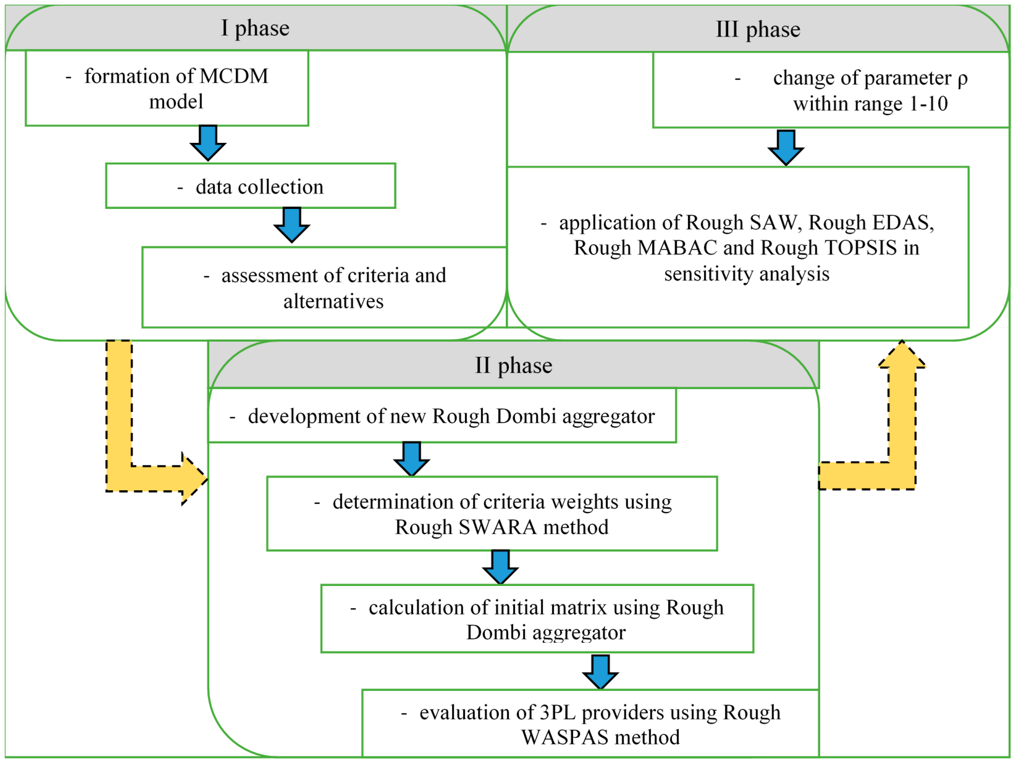
In addition to the introductory considerations, the paper is structured into an additional five sections. The second section presents a review of the state of the sector, with an emphasis on the last few years. The third section consists of algorithms of the applied methods. The algorithm of the new RDWGA operator is presented, as well as the steps of the Rough SWARA and the Rough WASPAS methods. The fourth section describes a case study and details calculation of the applied methods and aggregators. The fifth section presents a sensitivity analysis in three parts, while in the sixth section, conclusions are drawn with an emphasis on the contributions made and future research.
2. Literature Review
Transportation is one of the dominant logistics processes in a supply chain [
23,
24], and the increasing demand for transport services is a growing trend [
25]. The main reasons for this are: an increase in the volume and division of labor, the transfer of part of the production process to suppliers, seasonal fluctuations, different quantity orders, more frequent deliveries, and others. In most logistics systems, the share of transport costs in total costs is significant [
26]. In today’s environment, efficient transport is a competitive advantage, with many companies now focusing on optimizing logistics functions [
27]. Low costs, short transport times, and an acceptable level of risk are all challenges for logistics managers.
For many companies, the cost of transport is the highest logistics cost [
28]. In order to rationalize costs, the logistics sector will adopt a strategy to develop the company’s transport sector [
29,
30] and make a business decision: to possess its own vehicle fleet, hire a 3PL provider, or use both options depending on the relevant needs [
31]. Possessing its own vehicle fleet is a cost-efficient option if the available capacity of the vehicles is continuously used, which further causes a high cost of bound capital [
32].
The use of logistics providers is a function in which a company hands over one or more different elements of its supply chain to a 3PL provider [
33]. A third-party logistics (3PL) provider is an external provider that manages, controls, and delivers logistics activities on behalf of a shipper [
34]. This implies that the provider is capable of carrying out transport, customs clearance, storage, distribution of goods, and other logistics activities for clients [
35]. According to Langley [
3], the most popular activities to outsource are domestic transportation (80%), warehousing (66%), international transportation (60%), freight forwarding (48%), and customs brokerage (45%).
Research in the area of 3PL began to significantly appear in 1994 [
36] and has since then slowly grown. The external supply of logistics services is part of a trend toward outsourcing logistics activities [
37]. The scope of 3PL may range from a relatively limited combination of activities (e.g., transport and warehousing) to a comprehensive set of logistics services. Bhatnagar et al. [
38] lists the decision-making factors for choosing “3PL” providers and the main reasons for “3PL” activities: cost savings (86.8%), customer satisfaction (76.3%), and flexibility (75%). A key reason for such outsourcing is that with intensified global competition, companies are concentrating their energies on core activities that are critical for survival, and leaving the rest to specialist firms [
39]. Batarlienė and Jarašūnienė [
40] undertook research on 3PL that seeks to present the influence of 3PL on companies, as well as how to choose the key factors for optimizing business. They cite two main reasons for companies choosing to hire a logistics provider, which are: the company’s business being in trouble or the company’s rapid development, which subsequently necessitates seeking additional opportunities to improve business performance. In the evaluation and selection of 3PL providers, methods classified in different groups have thus been applied: decision-making techniques, statistical approaches, artificial intelligence, and mathematical programming [
41,
42,
43,
44,
45,
46,
47,
48,
49].
The paper examined the evaluation and selection of 3PL providers for the transport of hazardous substances in the chemical industry. Although there are many studies about the selection of 3PL providers, studies related to 3PL provider selection for the transport of dangerous goods are scarce. The selection of 3PL providers for the transport of dangerous goods is especially specific because of the inevitable risks that arise [
50] and the additional requirements that must be met by transport companies [
51].
The results of studies carried out by Leroux et al. [
52] with 106 companies handling dangerous materials show that transport activities are generally outsourced. Hanqing and Ru [
53] formed a 3PL mathematical model for the treatment of electrical waste and electronic equipment, as a class of dangerous goods.
Eroğlu et al. [
54] demonstrated an approach for determining the criterion importance degree in the 3PL provider selection process for the transport of dangerous materials, with the example of fuel as a multi-criterion decision-making (MCDM) problem. Bali and Eroğlu [
55] conducted studies on 3PL provider selection for dangerous materials. They developed a MCDM assessment model to select the most suitable 3PL provider using fuzzy DEMATEL and fuzzy TOPSIS. Fuzzy DEMATEL was used to determine weight of the criteria and fuzzy TOPSIS was used to evaluate alternative 3PL providers. Finally, Eliacostas [
56] wrote about the perspective of using 3PL providers for the safe routing of dangerous goods transport.
Evaluation and selection of Third-party logistics provider is one of very important areas for all participants in the supply chain. A large number of MCDM approaches is proposed for solving this problem in recent years. In [
57] integrated approach consists of fuzzy SWARA and fuzzy COPRAS for sustainable third-party reverse logistics provider selection is proposed. Fuzzy SWARA in combination with fuzzy MOORA is proposed in [
58] for third-party reverse logistics provider (3PRLP) evaluation. The authors of [
59] developed a novel integrated model consisting of fuzzy DEMATEL and fuzzy TOPSIS methods that helps companies to evaluate and select an appropriate logistics provider. Improving the quality of service, increasing the efficiency, and decreasing the cost, according to Ecer [
60], can be achieved through the proper selection of a logistics provider. In this research, he demonstrated a novel approach that integrated Fuzzy AHP and EDAS method. In [
61], a real-life case study in a confectionary company is presented to demonstrate the potential use of an integrated model that consists of fuzzy AHP and fuzzy TOPSIS methods. In that study, a model is proposed to provide a systematic decision support tool for 3PL provider evaluation, especially for a 3PL transportation provider. The authors of [
62] combined the cumulative prospect theory, the PROMETHEE II method, and a knowledge of thermodynamics to solve hesitant fuzzy linguistic MCDM problems. They solved the problem of green logistics provider selection. The same problem was also solved in [
63,
64]. To select the preferred service provider, the authors of [
63] used a hybrid method combining a variant of ELECTRE I accounting for the effect of reinforced preference, the revised Simos procedure, and Stochastic Multi-criteria Acceptability Analysis. In [
64], the authors extended the ELECTRE method and proposed a new methodology for handling fuzzy multi-criteria decision-making problems based upon interval type-2 fuzzy sets. Awasthi and Baležentis [
65] developed a hybrid model for logistics service provider selection, which consists of three phases. In the first phase, the authors identified the selection criteria using four categories: benefits, costs, opportunities, and risks (BOCR). The second phase involves generating linguistic ratings for potential partners on identified criteria by a committee of decision-making experts. In the third phase, the final partner selection is done using fuzzy MULTIMOORA. The importance of this area is also demonstrated in [
66], wherein the authors developed a novel integrated approach based on the CRiteria Importance Through Inter-criteria Correlation (CRITIC) and Weighted Aggregated Sum Product ASsessment (WASPAS) methods for the evaluation of 3PL providers with IT2FSs.
Evaluating 3PL providers for the transport of dangerous goods is rare, so this is one motivation for the execution of this research.
5. Sensitivity Analysis
The sensitivity analysis was carried out in three parts. The first part relates to the change of parameter
ρ, which changes within a range of 1–10, which means that a total of 10 scenarios were formed, whereby in each scenario parameter
ρ increases by one.
Table 10 shows the ranks of alternatives when changing parameter
ρ.
Table 10 shows that a change in parameter
ρ does not significantly affect the rank of alternatives. The only change occurs with alternatives four and five, which shift places. Alternative four is in in the fifth position the first three scenarios, while in the other scenarios, with the rise in parameter
ρ, it occupies the sixth position. It is important to note that a change in this parameter, or rather its increase, effects an increase in coefficient
λ, whose value surpasses one.
The second part of the sensitivity analysis implies the application of other methods in rough form to check the stability of the model and the results obtained. For these purposes, the following methods were used: Rough SAW [
72], Rough EDAS [
73], Rough MABAC [
20], and Rough TOPSIS [
8].
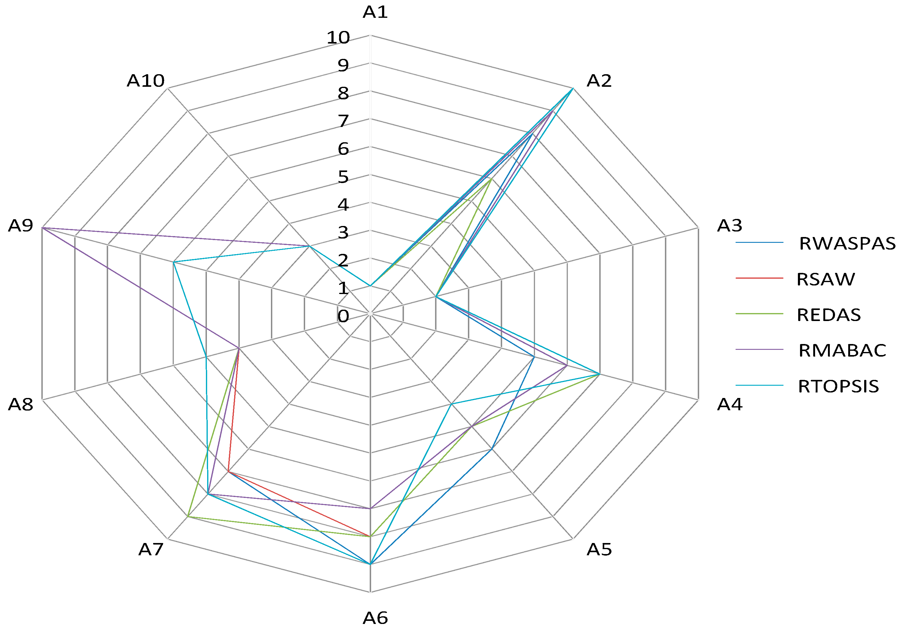
Looking at
Figure 2, we can perceive the stability of the obtained results, because even though different methods were applied, the first three positions do not change. The first, third, and tenth alternatives are placed in the first, second, and third places, respectively. The fourth position is filled by alternative eight through all approaches except the Rough TOPSIS, where it fills the fifth position. The fifth alternative is in the fifth position five times through application of the Rough SAW, Rough EDAS, and Rough MABAC, while the Rough WASPAS method places it sixth and the Rough TOPSIS in fourth place. In addition to the aforementioned alternative five, the sixth position contains alternatives four (Rough SAW and Rough MABAC), two (Rough EDAS), and nine (Rough TOPSIS). The biggest changes in rankings are seen in alternative two, which does not retain its position at any one time and as such ranked in the sixth, eighth, ninth, and tenth positions. The worst alternative is nine, which through calculation with four methods finds itself in last (tenth) place, with only the Rough TOPSIS method placing at sixth place.
The third part of the sensitivity analysis is the application of Spearman’s correlation coefficient (
Table 11) to determine the correlation of the ranks. Since it is evident that the alternative ranks are almost completely correlated in the first part of the sensitivity analysis, Spearman’s correlation coefficient was applied only to the second part of the sensitivity analysis, or in the calculation using different approaches.
Based on the total calculated statistical coefficient of correlation (0.971), it can be concluded that the ranks are in high correlation using different methods. When it comes to Rough WASPAS rank correlation with other methods, the lowest correlation is with Rough TOPSIS (0.927), because there is a difference of seven places in ranking, where the highest is in the ranking of the ninth alternative. The next lowest correlation is with Rough EDAS (0.939), because the difference in rank is in alternatives two, four, and seven by two places. There is a higher correlation of ranks with Rough MABAC (0.958) or Rough SAW (0.976), with fewer changes in ranks. The only major change in the ranking is with alternative six, which placed better by two places at Rough MABAC, in relation to the original position obtained by using Rough WASPAS. The Rough SAW has a slightly higher overall correlation coefficient (0.977) with other methods than Rough WASPAS, which means that there are small differences in ranks compared to other methods. The biggest difference is in comparison to Rough EDAS, where alternative two changed rank from ninth to sixth place. Rough EDAS has the lowest correlation coefficient (0.941). Observing the overall ranks and correlation coefficients, it can be concluded that the resulting model is very stable, and the ranks are almost completely correlated since, according to Keshavarz Ghorabaee et al. [
74], all values greater than 0.80 represent a very high correlation of ranks.
6. Conclusions
The transport of dangerous goods and its potential consequences arouses public attention because of these materials’ detrimental effect on the environment and people, as well as possible accidents. In order to meet the complex demands of today’s market, a trend of increased consumption of hazardous substances has appeared, thereby increasing the volume of production and transportation of these goods. Transport is a mandatory logistical activity for supplying users with these materials, regardless of whether they are in raw, semi-processed, or fully processed form.
In the midst of their companies’ accelerated development, an increasing number of dangerous substance manufacturers are trying to improve business performance and use the services of a 3PL provider. This study has developed a model that will make it easier for chemical industry companies to evaluate and select 3PL providers for the transport of dangerous goods. The Rough SWARA-WASPAS model, based on new Rough Dombi aggregators, was designed. A sensitivity analysis, carried out in three parts, confirmed the results of the proposed model.
The criteria defined for evaluating logistics providers are specific to the field of dangerous substances, due to the high risks [
75] and additional security requirements. One of the benefits of using the services of 3PL carriers is that they have a wider range of operations and are able to satisfy clients who have a high frequency of transport needs on a weekly basis. Specialized carriers better understand the market and customer needs. They also have well-designed strategies and business models to continue improving their offers, regional coverage, and specialization in all industry sectors.
During the course of research, “critical points” in the use of 3PL providers were identified. They are: lack of and unreliable information from the field, flow of documentation, physical flow of reverse logistics (if it exists), company presentation to the customer, slow problem-solving during delivery, and others.
A direction of further study is to support the environmental sustainability of 3PL dangerous material providers, particularly in areas that have been marked as topic areas [
76]: influencing factors, green actions, impact on performance, information and communication technology (ICT) tools supporting green actions, energy efficiency in road freight transport, and shipper’s perspective and collaboration. Another line of research may be the application of current MCDM methods for the evaluation and selection of 3PL providers for other logistics activities.


