Early CU Depth Decision and Reference Picture Selection for Low Complexity MV-HEVC

Abstract

The Multi-View extension of High Efficiency Video Coding (MV-HEVC) has improved the coding efficiency of multi-view videos, but this comes at the cost of the extra coding complexity of the MV-HEVC encoder. This coding complexity can be reduced by efficiently reducing time-consuming encoding operations. In this work, we propose two methods to reduce the encoder complexity. The first one is Early Coding unit Splitting (ECS), and the second is the Efficient Reference Picture Selection (ERPS) method. In the ECS method, the decision of Coding Unit (CU) splitting for dependent views is made on the CU splitting information obtained from the base view, while the ERPS method for dependent views is based on selecting reference pictures on the basis of the temporal location of the picture being encoded. Simulation results reveal that our proposed methods approximately reduce the encoding time by 58% when compared with HTM (16.2), the reference encoder for MV-HEVC.

1. Introduction

High Efficiency Video Coding (HEVC) is the latest video compression standard, introduced in 2013. When compared to H.264, HEVC offers almost double the compression ratio with nearly the same video quality [1]. Moreover, HEVC supports resolutions up to $8192\times 4320$ pixels, which is essential to important applications, such as augmented reality, live streaming, and HD video conferencing. With the development of fast Internet, mobile networks, video-enabled devices, and video-sharing websites, the data traffic is rapidly shifting towards video content. By the year 2022, 82% of all the data traffic is expected to be video data [2]. Therefore, video will play a dominant role in deciding the future of Internet and consumer devices. Video content generates a huge amount of data, especially when the resolution of the video is high. As video is a sequence of frames/pictures being displayed at a certain frequency, there is a high similarity between the pictures and within a picture in video data. Utilizing these characteristics of the video data, compression algorithms have been developed [3]. An encoder generally exploits the spatial and temporal correlation among the video data to reduce the number of bits in which the video information is stored. Video data in compressed form are sent over the network, and the receiver has to decode the compressed data to get the original video. Therefore, both the sender and receiver need to agree upon an encoding algorithm. To address the aforementioned issue, video compression standards have been developed [4]. These standards define the compression procedure, so that the consumer devices at the receiver end can reliably decode the compressed video. There are two main research fields in video coding, which are (i) the compression efficiency, which is a measure of the number of bits required to send a certain amount of video content. More information in a lesser number of bits corresponds to higher compression efficiency of a standard and (ii) encoder complexity, which is a measure of time required to encode a certain amount of video. Encoder complexity becomes very important in scenarios where the video information is required to be sent in a shorter span of time. With the rapid development of stereoscopic and auto-stereoscopic displays [5,6], multi-view and 3D video is gaining more popularity. Hence, recent standards also address this type of video data. H.264 has a multi-view extension known as Multi-view Video Coding (MVC) [7], and HEVC has MV-HEVC. The multi-view extensions of the standards use the multi-view video concept in which multiple cameras capture the same scene. The concept of Free View point Video (FVV) [8,9] also needs multi-view videos for virtual view synthesis [10]. In addition to the main standard, in the multi-view extension, the inter-view similarity of the video content is also exploited to get more compression. This further increases the encoding complexity. Therefore, more time is required to encode the videos in this format. Our work is one of the latest additions in the aforementioned domain in which we propose two techniques to reduce the encoding complexity of the encoder. The main contribution of our works are listed below.

• We propose an Early Coding Unit (CUs) Splitting (ECS) method, which is based on Coding Unit (CU) splitting information available from the base view. Moreover, the neighborhood of the co-located Coding Tree Unit (CTU) of the base view is used to derive the threshold depth for current CU in dependent views. This threshold depth value is further improved in the Temporal Level (TL)–4 of the pictures.
• We present an Efficient Reference Picture Selection (ERPS) method, in which we avoid the pictures in the reference pictures’ list, which are least probable for prediction. The proposed ERPS method also works in TL–4 because the reference pictures available have minimum temporal distance at this stage.
• We believe that the proposed ECS and the ERPS strategies provide much better performance for various sequences than previous published works.

The rest of the paper is structured as follows. Section 2 presents a brief overview of the related works, while Section 3 familiarizes readers about the fundamentals of the splitting and mode selection procedures of the basic coding and prediction blocks. Section 4 explains the complexity measuring parameters for the encoder. Section 5 describes the proposed ECS and the ERPS methods and their initial evaluations for the defined parameters. Section 6 lists detailed results and comparisons with recent state-of-the-art methods. Finally, Section 7 concludes the work and hints towards future research directions.

2. Literature Review

Below, we briefly consider some important methods that have been proposed to reduce the complexity of HEVC. Shen et al. [11] used different methods, such as the Rate Distortion (RD) cost [12], Motion Vector (MV) distribution [13], and the Coded Block Flag (CBF) [14], to achieve low complexity. Utilizing the observation that the depth of the CUs is generally similar to its neighborhood, the depth of neighboring CUs is used to decide the depth of the CU that is currently being encoded [15,16,17,18,19,20,21]. Later, Shen et al. [15] proposed a complexity reduction solution by selecting prediction modes according to three regions based on motion activity. In their work, complexity was reduced by studying the correlation between the different levels of CUs and the neighborhood. In [18], the spatio-temporal correlation between the depth of CTUs was used to reduce the depth level of the current CU accordingly. In [19], the published work used the information of the consecutive frames and CU levels from co-located CUs to avoid certain depth levels. A fast CU decision method, based on the Markov Random Field (MRF), was proposed in [20], which uses the variance of the absolute difference-based feature for CU selection. The aforementioned works are based on the observation that the neighboring decisions are mostly similar in a picture and also in co-located regions of available reference pictures. It is important to state here that all the pictures do not have similar partition decisions. Therefore, there are some regions normally referred to as boundaries, around which the partition decisions are not the same [13]. Few researchers have used RD cost for the early decision of CUs [22,23]. Lee et al. [22] proposed an RD cost-based fast CU decision method, which decides about the skip mode and CU splitting. Shen et al. [23] proposed three adaptive decision methods, which are early skip mode decision and two decision modes. One is based on prediction size correlation information, while the other is based on RD cost correlation. The aforementioned methods are well cited in the literature. However, they are not designed for multi-view videos.

In MV-HEVC, extra information from the previously-encoded view is also available for prediction. This aspect of multi-view videos of MV-HEVC was not exploited in the above-mentioned methods. MV-HEVC also considers inter-view prediction from co-located pictures of the base view. Therefore, its coding efficiency is further increased at the cost of increased encoding complexity. To the best of our knowledge, very few researchers have worked on reducing the complexity of MV-HEVC. In [24], the researchers proposed an inter-view prediction method for the HEVC-based multi-view video. The aforesaid work mostly used the maximum depth of the co-located CTU of the base view as the threshold for corresponding CUs of dependent views. Moreover, the researchers also encoded the multiple views separately as simulcast HEVC. The proposed method presented a nice idea for exploiting the inter-view correlation between the views, but it was limited to only the co-located CTU in the base view. Due to the disparity between the views, using only the co-located CTU is not a good option. We address this shortcoming in our proposed method by increasing the prediction window size in the base view. In [25], the authors introduced a fast CU decision algorithm. It predicts the depth of the current CU by determining a threshold depth value, which is calculated from the depth values of 1 inter-view co-located, 1 temporally co-located, and 3 neighboring CUs. MV information of the neighborhood CUs of current CU is used to correct threshold values calculated earlier. Due to the disparity between the views, the co-located CU of the base view is not a good option for predicting CU depth for dependent views. We address this issue in our proposed method, by using a larger area around the co-located CU. The temporally co-located CU used in [25] becomes ineffective due to motion and the temporal distance between the pictures. The three adjacent CUs used in [25] are only good when CUs (the CU being predicted and the CU being used for prediction) belong to the same object in the scene. We do not use adjacent CUs for predicting the depth threshold because this does not work when all the CUs involved do not belong to a single object. We also do not use temporally co-located CU; instead, we made use of temporal levels in our method. Recently, in [26], the published work predicted the CU depth of the dependent view through the depth decision made in the same region of the base view. Moreover, the prediction of the depth threshold is achieved by nine CTUs instead of using the CU neighborhood. It addresses the weakness of the method in [24]. In our proposed method, we further improve it by adding temporal levels to the threshold prediction. Whereas in [27], the authors suggested methods to implement encoding processes on parallel computing platforms, they also proposed a CU splitting termination method, which is based on Quantization Parameter (QP) values. Their algorithm is based on the observation that, with the increase in the QP value, the chances of CU splitting decrease.

The aforementioned works are nice efforts in the domain of MV-HEVC. However, we observed that still, many aspects of the correlation between the splitting and mode decision of a CU are not exploited. Therefore, our study mainly handles the aforementioned issue and exploits some of these areas. Below, we briefly introduce some basics of the standard, so that the reader can become familiar with the terminology used in the following sections.

3. Fundamentals

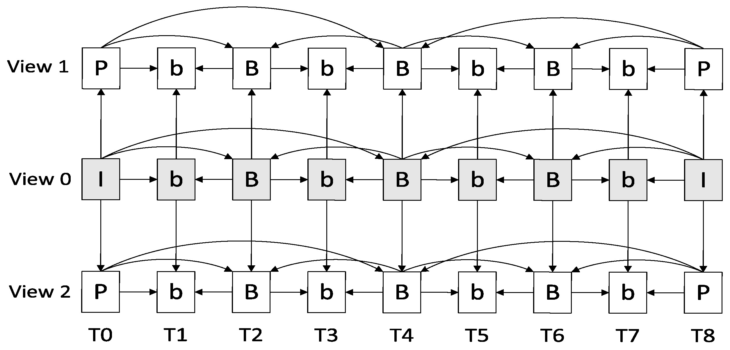
A typical prediction structure for three-view MV-HEVC is shown in Figure 1 in which View–0 is the base view that is encoded first without using inter-view prediction information. View–1 and View–2 are dependent views, as these use the inter-view prediction from the base view to improve the coding efficiency.

However, this increases the complexity of the encoder [28,29]. MV-HEVC uses the same basic prediction method and partitioning structure of the HEVC with the addition of using inter-view prediction. To be precise, the HEVC uses the quad tree partitioning structure [30,31,32,33]. The basic unit used for compression in HEVC is termed CTU, which can have a maximum size of $64\times 64$. This maximum size can be controlled through the configuration file.

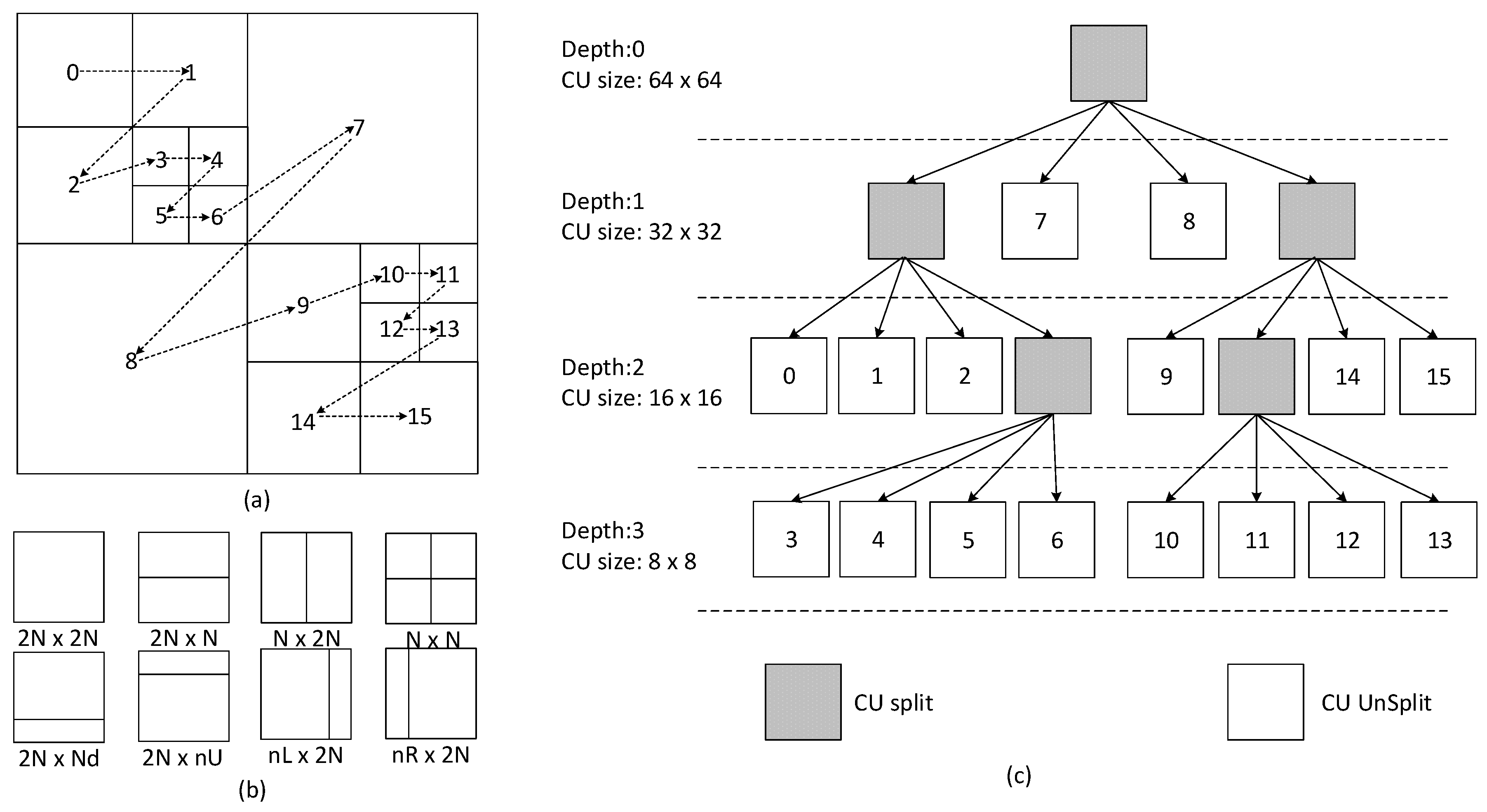
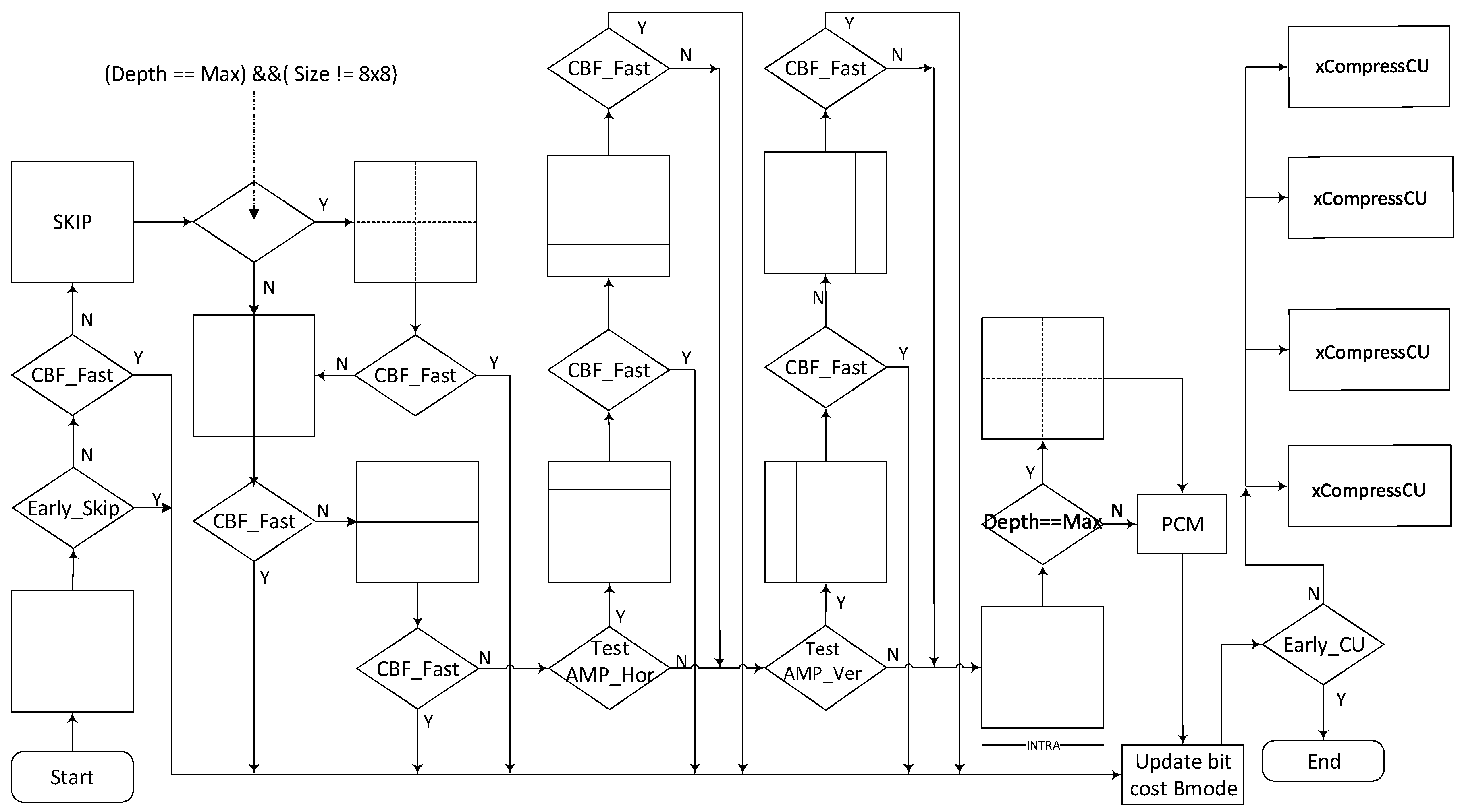
Figure 2a shows the splitting of a CTU into Coding Units (CUs), their processing order, and corresponding depth levels. Each CTU may contain a single CU or it may be split into four equally-sized square-shaped CUs. This process is continued until it reaches the minimum CU size of $8\times 8$. Each CU can be either predicted from previously-encoded reference pictures, that is inter-prediction, or from the same picture being encoded, which is intra-prediction. The CU can be further divided into a single or more Prediction Units (PUs). With a $2N\times 2N$ size of CU, the possible PU sizes are shown in Figure 2b. Intra-prediction only uses sizes $2N\times 2N$ and $N\times N$ for PUs, whereas inter-prediction uses all sizes for PUs. The use of size $N\times N$ is limited to the minimum CU size. The values for N: (32, 16, 8, 4) for the depth levels $D0,D1,D2,$ and $D3$, respectively as shown in Figure 2c. The CTU partitioning process of the HEVC is very complex. Therefore, most of the researchers have targeted simplifying this process. For example, Choi et al. [34] proposed an Early CU (ECU) decision method, which decides splitting on the basis of the current best mode decision of a CU depth. If the current best mode is determined to be skip mode, then further splitting is not done. Yang et al. [35] proposed a method that detects the skip decision early. This method is known as Early Skip Detection (ESD) in the related literature. Gweon et al. [36] proposed the CBF-based fast mode decision method. It stops splitting PUs when after the evaluation of a $2N\times 2N$ CU, the root CBF is zero. These methods are available in the HEVC reference encoder (HTM) as optimizing tools for low complexity HEVC. Figure 3 shows the CU and PU decisions’ process.

First, the cost for MODE-INTERwith a $2N\times 2N$ partition size is calculated. If it is activated, then the early skip condition is checked. If it is true, then the bit cost is updated, and other modes are left unchecked for the current depth. If it is not true, then the CBF-fast condition is checked. If this condition is true, then the bit cost is updated, and the best current mode is set to MODE-INTER with a $2N\times 2N$ partition. If this condition is not true, then the cost for MODE-SKIPis calculated and the mode cost is updated. Then, MODE-INTER with partition size $N\times N$ is calculated, after checking the depth and CU size requirements. Then, first, the mode cost for partition size $N\times 2N$ is calculated. Then, the mode cost for partition size $2N\times N$ is calculated and then Asymmetric Motion Partition (AMP) mode evaluation, according to

Table 1. Fast Asymmetric Motion Partition (AMP) mode evaluation [38].

Conditions	Actions
Best mode is ($2N\times N$)	Try $2N\times nU$ and $2N\times nD$
Best mode is ($N\times 2N$)	Try $nL\times 2N$ and $nR\times 2N$
Best mode is (($2N\times 2N$) && (!merge mode)&& (!skip mode))	Try all AMP modes
Parent CU is AMP mode	Only try merge mode for all AMP modes
Parent CU is (($2N\times 2N$) && (!skipped))	Only try merge mode for all AMP modes
Parent CU is ((intra) && (best mode is $2N\times N$))	Only try merge mode for $2N\times nU$ and $2N\times nD$
Parent CU is ((intra) && (best mode is $N\times 2N$))	Only try merge mode $nL\times 2N$ and $nR\times 2N$
CU size is $64\times 64$	No AMP modes are evaluated

. After every inter-partition, the CBF-fast method is applied. Meanwhile, inter-modes and intra-modes $2N\times 2N$ and $N\times N$ are checked. Mode $N\times N$ is only checked at the maximum depth. Then, before going to further splitting, the early CU condition is checked. The optimal depth selection for a CU and its thorough mode decision make the encoder very complex, which has attracted many researchers to find ways to reduce its complexity. The merge/skip mode is selected more than 88% [37] on average. Therefore, most researchers have targeted the early merge mode and early skip mode decision to achieve low complexity. Merge mode finds a PU from spatial and temporal merge candidates, whose motion information can be used for the current PU. If for the current PU, there exists such a PU in its merge candidates, whose transform coefficients and motion vectors are negligible, then it is coded with the skip mode. It is important to state here that the prediction residual is not transmitted in skip mode.

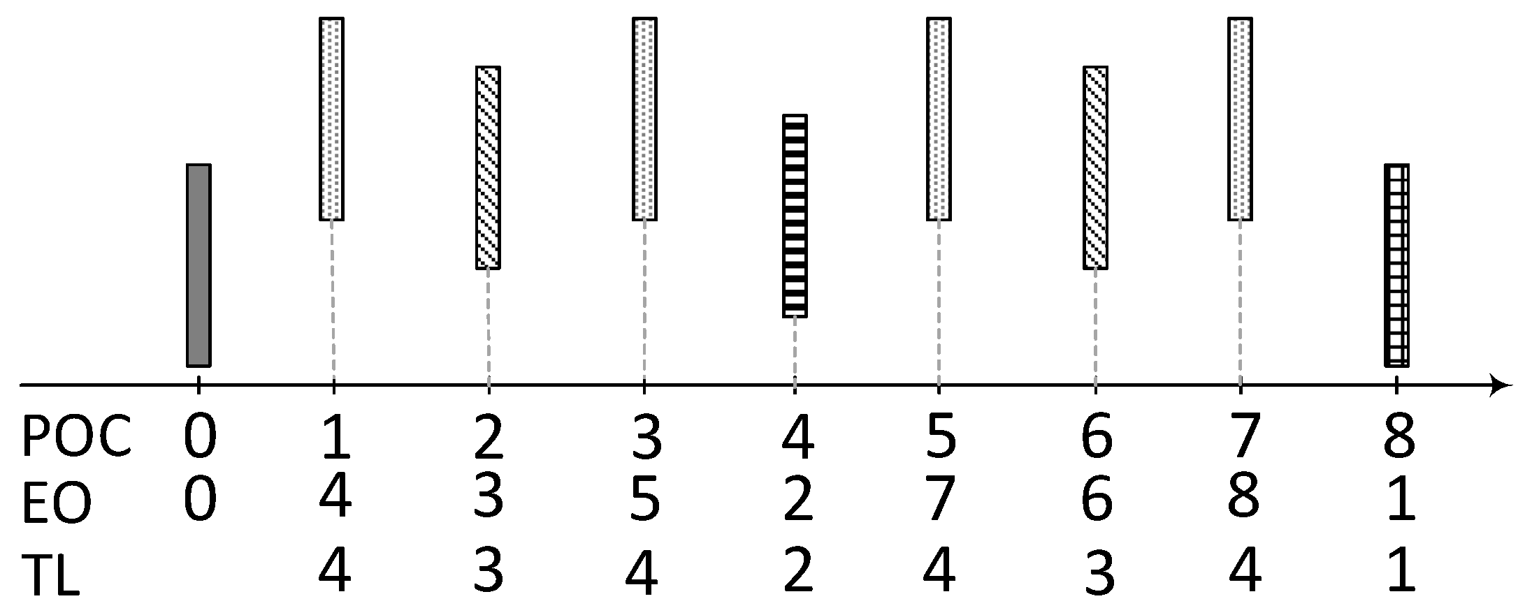
The video sequence of pictures is partitioned into coded video sequences, which can be decoded independently. Picture Order Count (POC) is the identification of a picture in the order in which the picture has been generated. Encoding Order (EO) is the order in which the pictures are encoded. Only the pictures that have already been encoded can be used for prediction. The coding structure defines the sequence of pictures, their POC, the EO, and the dependence between the pictures for prediction. The sequence of pictures in the coding structure is generally called the Group Of Pictures (GOP). In the HEVC literature, this set is normally referred to as the Structure Of Pictures (SOP). Figure 4 shows a GOP of eight pictures, with EO and POC. Pictures are grouped into different Temporal Levels (TLs). This division of pictures into TLs is based on the EO of the pictures and the POC of the available reference pictures. At TL–4, the availability of adjacent pictures for prediction is maximum. The decoded picture buffer contains the decoded pictures. Reference pictures are used from these decoded pictures. The reference picture set contains all the pictures that may be used for reference. For the prediction of the current picture, the reference pictures are stored in the reference picture list. There are two types of reference picture lists used in HEVC, which are List–0 and List–1. List–0 is used when the slice is of the P–type. For the B-type slice, both List–0 and List–1 can be used. For uni-prediction, List–0 or List–1 is used, and for bi-prediction, both Lists are used. Inside a reference picture list, the pictures are identified by the reference picture index. The pictures used as a reference from the reference picture lists are selected on the basis of finding the best available match. As the content of the video is mostly similar between consecutive pictures, there is a strong correlation between the pictures, which are located at a short temporal distance from each other. In the next section, we briefly overview the related works. In the next section, we briefly describe the complexity measuring parameters that have also been used in our proposed methodologies and evaluations.

4. Complexity Measuring Parameters

The computational complexity is due to the calculations of arithmetic functions used during the encoding process. According to the findings in [39], the functions, such as the Hadamard (HAD) transform, Sum of Absolute Difference (SAD), and Sum of Squared Error (SSE), are the main cause of the computational complexity. To measure the complexity reduction of our proposed method, we investigated these parameters. For a block, being encoded at the current size, its best match is searched, spatially, temporally, and in the base view within a search window. This process is repeated for each block size, all possible prediction modes, and for all possible search locations. The best match implies a minimum difference between the current block and its match from all the available options. Equation (1) shows how the difference between the current block and the predicted block of the same size is calculated.

$$Diff(i,j)=BlockA(i,j)-BlockB(i,j)$$

(1)

where i and j represent the location of the pixel. SSE and the SAD as described in Equations (2) and (3), respectively, are used to find the error between the blocks being encoded with its possible matches.

$$SSE=\sum _{i,j}Diff{(i,j)}^2$$

(2)

$$SAD=\sum _{i,j}\left|Diff(i,j)\right|$$

(3)

This process also needs to consider bit cost, which is the number of bits required to describe the splitting and prediction information. The overall cost functions for the prediction parameter and mode decisions are described in Equations (4) and (5), respectively. This is generally called Rate Distortion (RD) cost.

$$J_{pred,SAD}=SAD+{\lambda }_{pred}\ast B_{pred}$$

(4)

$$J_{mode}=(SS{E}_{lu.}+w_{ch.}\ast SS{E}_{ch.})+{\lambda }_{mode}\ast B_{mode}$$

(5)

where $B_{mode}$ and $B_{pred}$ are the bit costs for the mode and prediction decisions, respectively. ${\lambda }_{pred}$ and ${\lambda }_{mode}$ are Lagrange multipliers, and ${}_{lu}$ and ${}_{ch}$ stand for luma and chroma, respectively. $w_{ch}$ is the weighting factor for the chroma part of SSE. These processes are called each time, and a comparison is made to get the best match. The number of times a process is called during the encoding gives insight about the complexity of the encoding. In our comparison, we used these parameters to demonstrate the reduction in encoding complexity. To compare the complexity of the encoder in its original form with our proposed method, we use Equations (6)–(8) to get the percent reduction in these operations.

$$\mathsf{\Delta }HADs(\%)=\frac{HAD{s}_{(Orig.)}-HA{D}_{(Prop.)}}{HAD{s}_{(Orig.)}}\times 100\%$$

(6)

$$\mathsf{\Delta }SAD(\%)=\frac{SA{D}_{(Orig.)}-SA{D}_{(Prop.)}}{SA{D}_{(Orig.)}}\times 100\%$$

(7)

$$\mathsf{\Delta }SSE(\%)=\frac{SS{E}_{(Orig.)}-SS{E}_{(Prop.)}}{SS{E}_{(Orig.)}}\times 100\%$$

(8)

where “Orig.” means the values for the the original configuration of the reference encoder and “Prop.” means the values for the proposed method implemented in the reference encoder.

5. Proposed Methods

In this section, we explain our proposed complexity reduction methods in detail. In Section 5.1, initially, the proposed ECS method is explained step by step. Then, it is compared with the reference encoder in terms of percentage reduction in the selected operations. In Section 5.2, first, the proposed ERPS method is discussed followed by a comparison with the reference encoder. In all of our observations, analysis, and implementation, we used the standard test sequences as shown in

Table 2. Test sequences used in the analysis and results.

Test Sequence	Resolution	Input Views	Frames/Pictures
Balloons	1024 × 768	1-3-5	300
Kendo	1024 × 768	1-3-5	300
Newspaper	1024 × 768	2-4-6	300
GT_Fly	1920 × 1088	9-5-1	250
Poznan_Hall2	1920 × 1088	7-6-5	200
Poznan_Street	1920 × 1088	5-4-3	250
Undo_Dancer	1920 × 1088	1-5-9	250
Shark	1920 × 1088	1-5-9	300

. In places where the QP value is not mentioned, averaged values for different QP values (25, 30, 35, 40) are used.

5.1. Proposed ECS Approach

The selection of the best CU size is a time-consuming process because the encoder has to go through all possible combinations of sizes and available reference pictures for the selection of the best match on the basis of the minimum RD cost. If the CU size selection process can be reduced, the overall encoding time can be reduced considerably. Therefore, we target the early termination of CU splitting, based on the inter-view and temporal information available. The immediate question that arises is: is there any room for further optimization of the CU size selection process, i.e., if we can predict the maximum CU size early, would we be able to reduce the encoding time? In order to find an answer to this question, we want to know about the percentage relation between CTU depth levels.

Table 3. Average CU depth percentages of dependent views.

Sequence	Depth Levels (%)
	D0	D1	D2	D3
Balloons	69.1	23.8	5.9	1.3
Kendo	74.1	19.8	4.9	1.1
Newspaper	79.3	13.9	5.1	1.6
GT_Fly	70.1	19.2	8.5	2.1
Poznan_Hall2	84.5	12.2	2.3	1.1
Poznan_Street	82.8	12.2	3.8	1.2
Undo_Dancer	74.1	17.8	5.9	2.2
Shark	76.1	17.1	5.2	1.4
$1024\times 768$ (avg.)	74.2	19.2	5.3	1.3
$1920\times 1088$ (avg.)	77.5	15.7	5.1	1.6
Average	76.3	17.0	5.2	1.5

shows the percentage relation between the depth levels ($D_0-D_3$).

As it is evident in Table 3, a high percentage of CUs are best matched at the $D_0$ level, which is due to the fact that the major portion of a picture is similar. Table 3 gives us an answer to our question that, yes, there is a very small percentage (1.5%) of CUs that are best matched at Depth Level 3, and on average, 76.3% of CUs are matched at Depth Level 0, which means that if the maximum depth level of the majority of the CUs is predicted correctly, then the time-consuming splitting and matching process for higher depth levels can be saved.

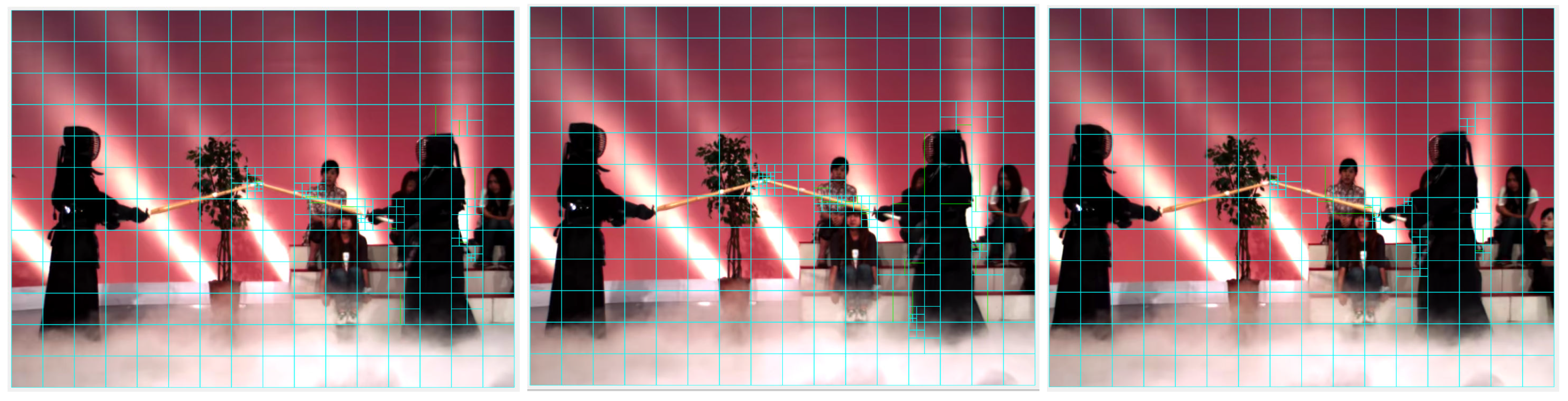
In multi-view video coding, different cameras capture the same scene, which means that the content of the videos is almost the same. The slight difference is due to the change in angle of capturing between the scene and the cameras. In other words, the decisions made by the encoder for multiple video streams of multiple cameras should also be very similar. This can also be observed from the CU splitting decisions shown in Figure 5. The CU splitting decisions in the same region between the pictures are very similar. This implies that much correlation exists between the views and corresponding regions of the picture. This is our motivation to use the CU splitting decisions of the same region of the base view to predict the CU depth threshold of the dependent views. By the same region in the base view, we mean a square area/window, centered onthe co-located CU of the dependent view. Adding this with the observations in Table 3, we build our ECS method.

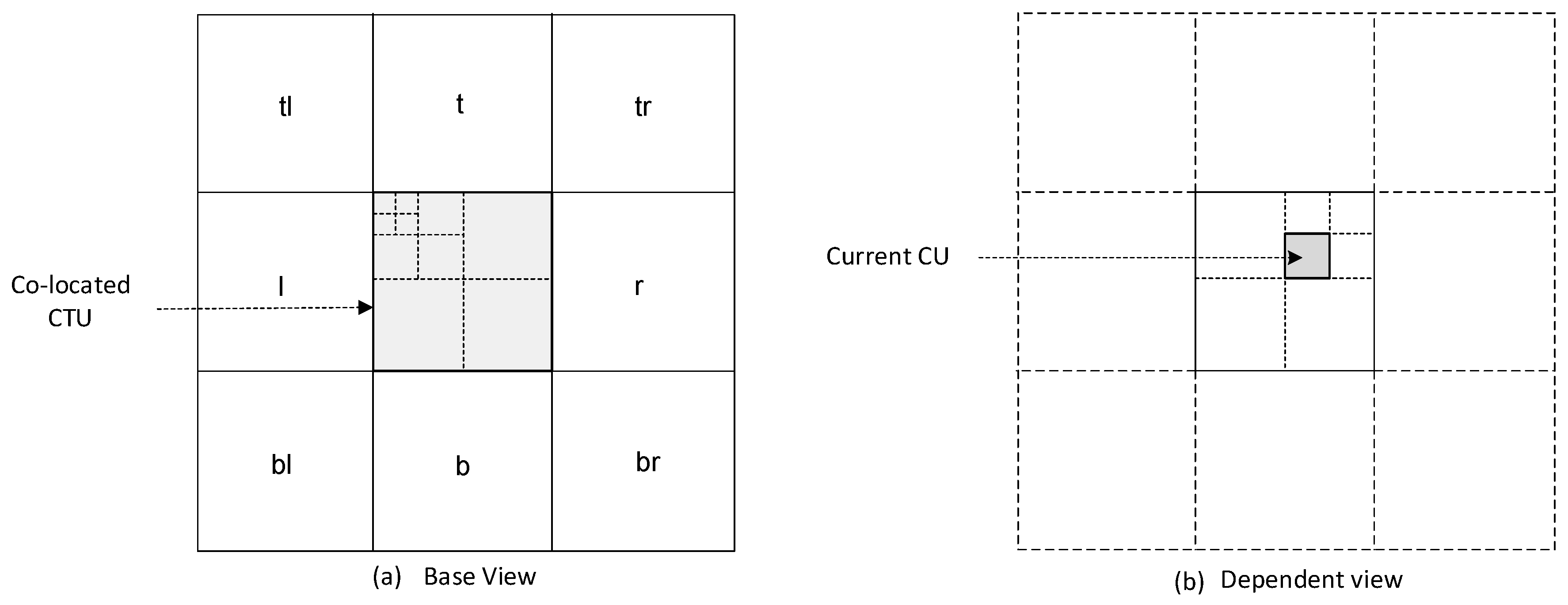
To get the depth threshold value for the CU being encoded in the dependent view, we used a window of 3 × 3 CTUs around the co-located CU in the base view. This is graphically shown in Figure 6. The CU, which is currently encoded as shown in Figure 6a, and its co-located CTU along with its neighborhood are depicted in Figure 6b. To get a broader observation area, the co-located CTU and its eight surrounding CTUs were considered in our analysis. CTUs of the base view were assigned the highest depth level of the CUs they contained after encoder decisions. As an example, the co-located CTU of the base view in Figure 6a contains 3 CUs of Depth Level 1, 3 CUs of Depth Level 2, and 4 CUs of Depth Level 3. As the highest depth level contained by this CTU was three, the depth level assigned to this CTU was three, i.e., $D_{Co}=3$. We define the depth threshold for the CU of dependent view based on the depth levels of the CTUs located in its co-located CUs neighborhood in the base view as $D_{r1}$ shown in Equation (9).

$$D_{r1}=max\left\{D_{tl},D_t,D_{tr},D_l,D_{Co},D_r,D_{bl},D_b,D_{br}\right\}$$

(9)

where, $D_{tl}$, $D_t$, $D_{tr}$, $D_l$, $D_{Co}$, $D_r$, $D_{bl}$, $D_b$, and $D_{br}$ are the maximum CU depths of the CTUs of the base view, as shown in Figure 6a.

Table 4. Hit–miss percentages.

Sequence	Outcome (%)
	Hit	Miss
Balloons	99.2	0.8
Kendo	99.4	0.6
Newspaper	99.6	0.4
GT_Fly	99.5	0.5
Poznan_Hall2	99.6	0.4
Poznan_Street	99.8	0.2
Undo_Dancer	99.7	0.3
Shark	99.6	0.4
$1024\times 768$ (avg.)	99.4	0.6
$1920\times 1088$ (avg.)	99.6	0.4
Average	99.6	0.4

gives us an idea of how accurately we can predict the depth threshold, in terms of “hit” and “miss”. If the depth of the current CU is higher than our assumed depth, then we call it a “miss”, otherwise it is called a “hit”. It can be seen from the results that the hit percentage is very high, which means that the predicted depth threshold $D_{r1}$ is highly accurate.

Table 5. Relation between the hit scenario and CU depths.

Test Sequence	Depth Levels (%)
	D0	D1	D2	D3
Balloons	48.23	11.94	8.62	31.24
Kendo	41.80	13.50	9.23	35.35
Newspaper	49.10	11.70	9.10	30.30
GT_Fly	51.40	14.10	11.20	23.30
Poznan_Hall2	52.30	14.10	10.30	23.50
Poznan_Street	49.80	13.10	8.70	28.50
Undo_Dancer	50.30	13.20	10.50	26.10
Shark	50.10	13.50	9.30	27.10
$1024\times 768$ (avg.)	46.38	12.38	8.98	32.30
$1920\times 1088$ (avg.)	50.78	13.60	10.00	25.70
Average	49.13	13.14	9.62	28.17

summarizes the percentages of depths of CUs in the case of a hit. If the CU depth is predicted at $D_{r1}=0$, then the chance to reduce complexity is highest, because the matching process for higher depths is avoided.

Similarly, if a depth level $D_{r1}=3$ is predicted for a CU, then it does not reduce the encoding complexity because the encoder has to go through all the depth levels.

After utilizing the inter-view correlation, now we move on to the temporal domain. It can be seen in Figure 4, at TL–4, that the adjacent pictures are available as reference pictures. Therefore, in this case, there is a very high probability that the scene has not changed and that the best match can be found at lower depth levels as compared with lower TL pictures.

Table 6. Relation of average CTU depth percentages with TLs of the pictures in dependent views.

TLs	Depth Levels (%)
	D0	D1	D2	D3
TL–1	59.83	15.36	10.66	14.13
TL–2	80.82	09.18	05.44	03.91
TL–3	87.43	07.16	03.31	01.99
TL–4	95.18	02.92	01.11	00.78

summarizes the relation between depth levels of CTUs and TLs. Here, CTUs are considered instead of CUs because CTUs are of the same size and have a constant number in each picture. Therefore, a CTU is considered at depth level $D_3$ when it contains at least one CU of depth level $D_3$, and a CTU is considered to be at depth level $D_2$ when it has at least one CU having depth $D_2$ and no CU with depth $D_3$. It can also be seen that at TL–4, above 95% of CTUs are at depth level $D_0$ and 98.1% of CTUs are at depth levels $D_1$ and $D_2$. Only 1.87% of CTUs have depth level $D_2$ and $D_3$. Therefore, for TL–4, we used $D_{r2}$ as the depth threshold, shown in Equation (10).

$$D_{r2}=\left\{\begin{array}{cc}0,\hfill & \mathrm{if}{D}_{r1}=0\hfill \\ D_{r1}-1,\hfill & \mathrm{Otherwise}\hfill \end{array}\right.$$

(10)

Table 7. Hit scenario relation of average CTU depths with TLs of the pictures in dependent views.

TLs	Depth Levels (%)
	D0	D1	D2	D3
TL–1	12.50	11.31	10.67	65.6
TL–2	36.80	16	11.32	35.92
TL–3	48.56	14.36	12.09	25.04
TL–4	71.64	11.58	7.08	9.71

shows the average CU depth relation with TLs in the case of the hit scenario. Here, we can see that a high percentage of CUs are at depth level $D_0$. These results are very attractive, but when we go through the details of the encoding process, the possible reduction in encoding complexity is not that much, as can be seen from these results. At TL–4, we find that most of the lower depth CUs are encoded in skip mode, which means that these CUs do not go through the time-consuming splitting and matching process for depth levels. Therefore, detecting these lower depths earlier does not play a significant role in the complexity reduction as the percentages of Table 7 are suggesting.

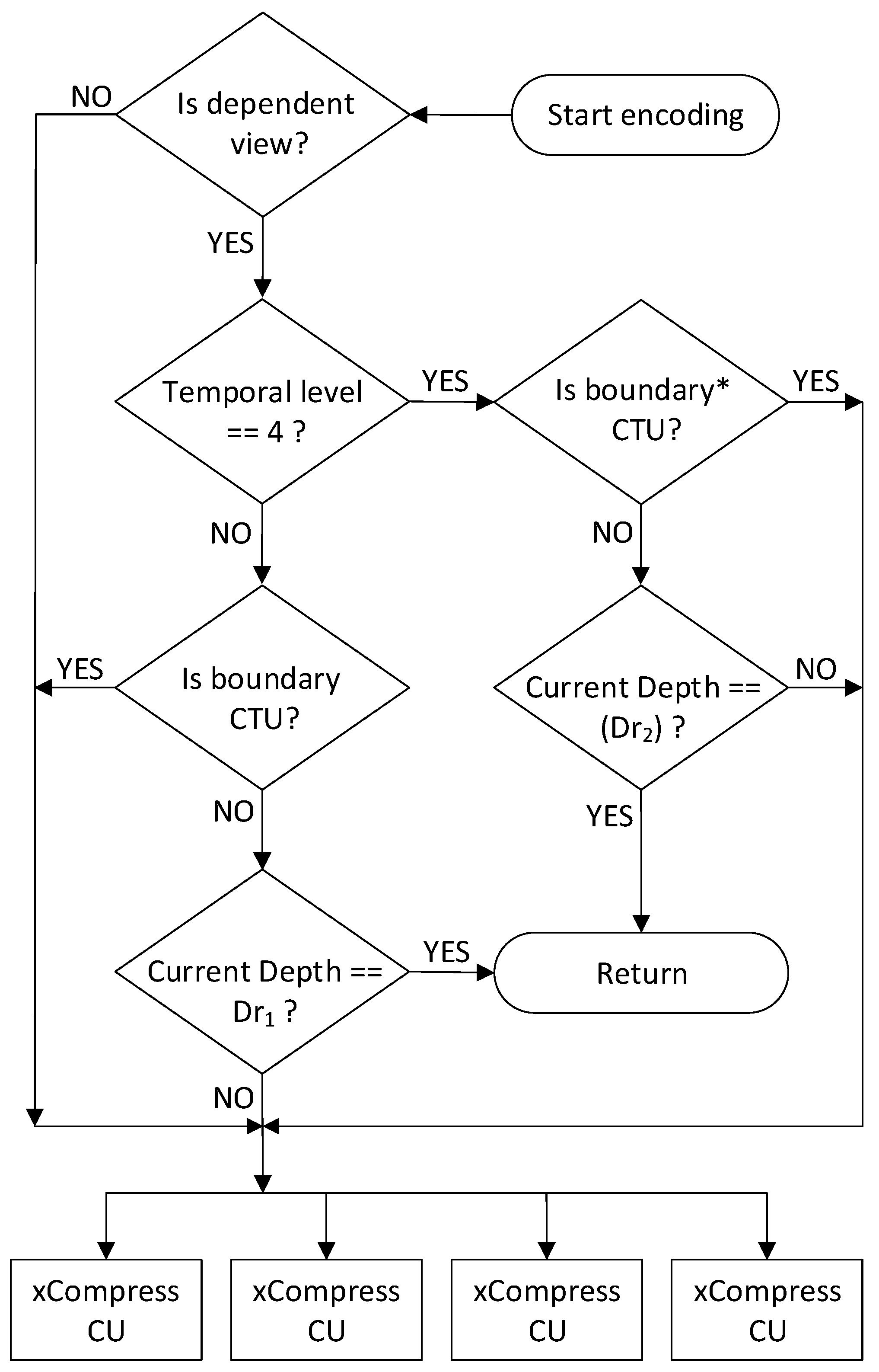
We propose an algorithm for early splitting of the CU. We call this new method ECS. Our algorithm is based on CU splitting information of the base view and CU splitting information related to the TLs of the pictures. The flow of the proposed ECS algorithm is shown in Figure 7. In our proposed method, we aim to reduce the complexity of dependent view encoding, where the base view is used for gathering information. Our proposed ECS method can be divided into two main parts. In the first part, we only deal with pictures that do not belong to TL–4. When the encoding for the dependent view starts, we first check whether the current CU belongs to a boundary CTU. If it belongs to a boundary CTU, then the normal encoding process is used. If it is a part of non-boundary CTU, then we compare it with the maximum depth threshold $D_{r1}$, as shown in Equation (9), which we have calculated for this CU from the base view. If the current CU depth is equal to the calculated depth threshold, then further splitting to higher depth levels of the CU is not done. In the second part, we deal with pictures that belong to TL–4. As shown in Table 6, at TL–4, the percentage of depth level $D_0$ is very high as compared with lower TLs. On the basis of this observation, we modified our method for TL–4. Therefore, we used depth threshold $D_{r2}$ Equation (10) for TL–4.

Operations with respect to sizes of the blocks are used as a comparison tool. It can be seen in

Table 8. ECS results in terms of percentage reduction of SAD, SSE, and Hadamard (HAD) operations.

Sequences	SAD								SSE					HADs
	SAD	4	8	16	12	24	32	64	SSE4	8	16	32	64	HADs	4	8
Balloons	3.6	74.8	73.8	68.8	4.2	3.3	54.5	−0.2	53.9	46.4	32.9	22.3	−0.1	72.5	73.0	48.0
Kendo	19.7	71.9	71.0	65.5	22.0	25.3	53.0	0.1	53.3	45.6	31.9	21.9	0.0	70.8	71.0	47.3
Newspaper	5.3	76.4	76.6	73.8	6.1	6.8	60.5	0.0	57.6	50.5	37.7	26.9	0.0	75.3	74.8	51.5
GT_Fly	26.4	79.8	79.0	73.4	29.9	27.1	57.2	0.4	67.8	60.8	46.4	32.7	0.0	78.5	79.1	52.5
Poznan_Hall2	19.3	85.5	85.0	80.0	20.2	18.6	62.3	0.0	69.3	61.1	45.0	31.0	0.0	82.8	83.8	55.7
Poznan_Street	22.7	74.5	73.9	69.4	26.9	31.1	57.2	0.9	57.8	51.0	37.7	26.6	0.0	73.8	73.6	49.8
Undo_Dancer	17.6	74.2	73.8	68.7	19.1	22.7	55.4	0.1	58.5	51.7	38.3	26.8	−0.1	72.6	71.9	48.6
Shark	31.4	72.8	71.8	66.8	35.0	34.2	54.1	1.3	61.6	54.4	40.1	27.6	0.1	73.7	74.4	48.6
1024 × 768 (avg.)	9.5	74.4	73.8	69.4	10.8	11.8	56.0	0.0	54.9	47.5	34.1	23.7	0.0	72.9	72.9	49.0
1920 × 1088 (avg.)	23.5	77.3	76.7	71.7	26.2	26.7	57.2	0.6	63.0	55.8	41.5	28.9	0.0	76.3	76.6	51.0
Average	18.2	76.2	75.6	70.8	20.4	21.1	56.8	0.3	60.0	52.7	38.8	27.0	0.0	75.0	75.2	50.3

that there is a significant decrease in the number of SSE, SAD, and HAD operations. To show the effect of resolution, average values of $1024\times 768$ and $1920\times 1088$ pixels sequences are separately calculated. It can be seen that in the case of the SAD64 and SSE64 operations, the percentage reduction in operations is very low, which means that the CUs at depth level $D_0$ are not reduced. The highest percentage decrease in SAD operations can be observed at SAD4 and SAD8, which is on average 76.2% and 75.6%, respectively. These are followed by SAD16 and SAD32, which on average are 70.8% and 56.8%, respectively. The percentage reduction in operations SAD12 and SAD24 is comparatively low. A similar pattern can be observed in the percentage reduction of SSE and HAD operations, where the percentage reduction in operations decreases with the increase in the size of the block. This happens because we are trying to reduce the splitting process, and in comparison with the original encoder, the lower depth levels of CUs are mostly avoided in our proposed method. We get the higher percentage reduction in operations, which are related to higher depth levels. It can also be seen that this phenomenon is independent of the video content. These results give us a general view of the complexity reduction of the encoder, as we can see for the percentage reduction of the operations. The size of the operation block is directly proportional to the amount of time the operation takes. Therefore, the high percentage reduction in smaller block size operations might not be reflected as much in the overall encoding time.

5.2. Proposed ERPS Approach

Since video is a sequence of pictures captured in discrete time intervals, these pictures contain many similar contents. The encoder uses this aspect to compress the video data. The encoder maintains a set of encoded frames/pictures as reference pictures for the picture being encoded. This set of reference pictures is selected on the basis of EO and temporal distances. Some pictures in reference lists may be temporally near and some may be far from the picture being encoded. As video is a sequence of discrete pictures in the time domain, the content similarity between the pictures of the video is inversely proportional to the temporal distance between the pictures. Based on this characteristic of video and the video encoder, we built our reference picture selection method. At TL–4 for a picture being encoded, the immediate previous and next pictures are available in the reference picture list. There is a very high probability that these adjacent pictures might be selected as reference pictures rather than a picture, which is at some temporal distance from the picture being encoded.

To further strengthen our argument, the correlation among these pictures, the reference picture selection in terms of the reference indices of both reference lists is analyzed. Moreover, we want to know which pictures are referenced mostly for encoding each picture, so that we can avoid the matching process for the reference pictures that are least expected to be selected as the reference picture. We performed the analysis for both the reference picture lists. We divided our analysis result on the basis of TLs, as shown in Figure 4.

Table 9. Reference indices selected as a percentage for both List–0 and List–1 for different TLs.

Ref. List	Sequences	TLs of Pictures with Reference Picture Indices
		TL–1		TL–2			TL–3			TL–4
		Index–0	Index–1	Index–0	Index–1	Index–2	Index–0	Index–1	Index–2	Index–0	Index–1	Index–2
List–0	Balloons	66.88	33.12	62.20	26.83	10.98	87.83	5.27	6.90	98.78	0.70	0.52
	Kendo	38.61	61.39	63.84	27.91	8.25	73.76	10.72	15.52	91.60	2.25	6.15
	Newspaper	79.01	20.99	65.84	6.45	27.71	97.36	1.69	0.95	98.69	1.01	0.30
	GT_Fly	1.90	98.10	4.14	94.71	1.14	34.41	30.36	35.24	70.59	7.10	22.31
	Poznan_Hall2	56.78	43.22	75.00	11.46	13.54	83.77	3.50	12.73	95.77	2.74	1.49
	Poznan_Street	49.39	50.61	58.79	33.93	7.28	61.87	16.36	21.76	76.16	8.19	15.65
	Undo_Dancer	22.00	78.00	56.05	35.36	8.59	70.91	15.06	14.03	82.28	8.50	9.21
	Shark	1.02	98.98	4.87	93.97	1.15	15.13	42.36	42.51	39.38	16.28	44.34
	1024 × 768 (avg.)	61.50	38.50	63.96	20.40	15.64	86.32	5.90	7.79	96.36	1.32	2.32
	1920 × 1088 (avg.)	26.22	73.78	39.77	53.89	6.34	53.22	21.53	25.25	72.84	8.56	18.60
	Average	39.45	60.55	48.84	41.33	9.83	65.63	15.67	18.70	81.66	5.85	12.50
List–1	Balloons	80.33	19.67	61.28	38.72	0.00	93.58	0.11	6.31	98.20	1.05	0.75
	Kendo	68.87	31.13	57.11	41.72	1.17	78.65	4.30	17.05	98.09	1.52	0.39
	Newspaper	86.49	13.51	71.26	28.45	0.29	95.52	0.10	4.38	98.10	1.05	0.85
	GT_Fly	76.58	23.42	3.86	93.71	2.43	41.58	0.71	57.71	98.96	1.01	0.03
	Poznan_Hall2	74.37	25.63	68.75	30.73	0.52	82.02	1.34	16.64	98.13	1.12	0.75
	Poznan_Street	82.87	17.13	50.56	47.98	1.46	66.81	2.92	30.27	98.06	0.42	1.52
	Undo_Dancer	70.02	29.98	50.08	46.32	3.60	77.31	3.86	18.84	93.27	4.60	2.13
	Shark	62.44	37.56	2.78	96.41	0.81	26.99	0.70	72.31	98.21	1.01	0.78
	1024 × 768 (avg.)	78.56	21.44	63.22	36.30	0.49	89.25	1.50	9.25	98.13	1.21	0.66
	1920 × 1088 (avg.)	73.26	26.74	35.21	63.03	1.76	58.94	1.91	39.15	97.33	1.63	1.04
	Average	75.24	24.76	45.71	53.00	1.29	70.31	1.75	27.94	97.63	1.47	0.90

illustrates our analysis of reference indices in terms of the percentage for List–0 and List–1 for various temporal levels. It can be observed from these results that for List–1, at TL–4, the selection of both reference Index–1 and Index–2 is less than 2.5%, while Index–0 is selected 97.5%. Now, our logical argument is also backed up by practical results. Reference picture selection is dependent on the temporal relation between the picture being encoded and the picture being referenced for prediction. Now, using the observations in Table 9, we can reduce the computation complexity by avoiding the search and matching process for reference Index–1 and Index–2 in List–1. During the encoding process when the TL of the picture being encoded is 4, then we do not use the reference pictures indexed as 1 and 2 in reference picture List–1, only the reference picture, which is indexed as 0 in List–1, used as the reference picture option. For pictures that do not belong to TL–4, normal encoding process is followed.

Algorithm 1 shows the pseudo-code of the proposed ERPS method in the encoding process, which processes the TL of the picture being encoded and outputs List–1, which contains Index–0, Index–1, and Index–2, as shown in Algorithm 1.

Algorithm 1 Proposed ERPS algorithm

Table 10. Efficient Reference Picture Selection (ERPS) results in terms of the percentage reduction of SAD, SSE, and HAD operations.

Sequences	SAD								SSE					HADs
	SAD	4	8	16	12	24	32	64	SSE4	8	16	32	64	HADs	4	8
Balloons	0.3	11.0	16.4	16.4	0.2	0.7	14.4	11.9	0.0	0.0	0.0	0.1	0.1	13.6	10.5	15.7
Kendo	17.2	12.5	16.8	16.6	18.5	24.0	15.8	13.4	0.4	0.6	1.0	1.3	1.1	13.5	11.4	15.8
Newspaper	2.0	10.6	17.2	17.8	1.9	3.6	14.7	10.8	0.0	0.1	0.1	0.2	0.2	14.3	10.6	17.0
GT_Fly	13.2	12.6	18.8	19.7	12.3	17.5	19.1	18.2	0.2	0.4	0.9	1.1	1.2	14.2	11.3	17.1
Poznan_Hall2	4.8	11.9	17.2	16.7	3.9	6.9	13.9	11.4	0.1	0.1	0.2	0.3	0.4	13.7	10.9	15.8
Poznan_Street	20.3	12.9	18.7	19.7	22.8	29.4	19.0	15.5	0.4	0.6	1.1	1.4	1.2	14.4	11.6	17.4
Undo_Dancer	13.4	12.2	17.5	17.9	13.6	19.5	17.1	14.4	0.5	0.7	1.2	1.4	1.4	13.9	11.3	16.5
Shark	25.7	13.6	18.4	19.9	26.9	31.3	20.4	19.3	0.5	1.0	1.9	2.4	2.4	14.4	12.0	17.9
1024 × 768 (avg.)	6.5	11.4	16.8	16.9	6.8	9.4	15.0	12.0	0.1	0.2	0.4	0.5	0.5	13.8	10.8	16.2
1920 × 1088 (avg.)	15.5	12.6	18.1	18.8	15.9	20.9	17.9	15.8	0.3	0.6	1.0	1.3	1.3	14.1	11.4	17.0
Average	12.1	12.2	17.6	18.1	12.5	16.6	16.8	14.4	0.3	0.5	0.8	1.0	1.0	14.0	11.2	16.7

shows the results’ comparisons obtained by our proposed ERPS algorithm with HTM $\left(16.2\right)$. We compare both on the basis of the number of SAD, SSE, and HAD operations done in each configuration of the encoder. The results in Table 10 show the percentage reduction in the number of these operations by our proposed ERPS method with respect to the HTM $\left(16.2\right)$ encoder configuration using Equation (7). In the case of the SAD operation, the percentage reduction for sizes 8, 16, 32, and 64 generally shows a similar trend. This means that reference picture selection does not affect a particular size operation, as was observed in the case of the ECS. The percentage reduction for these sizes is also observed to be independent of the video content. It can be seen that the percentage decrease in the SAD and the HAD operations is somewhat similar, but the percentage decrease in the SSE operations is very low. From Equations (4) and (5), we see that the SAD operation is called in the cost function for the prediction parameter decision, and the SSE operation is called in the cost function for the mode decision. The prediction parameter decision process is simplified due to our proposed ERPS method. Therefore, the effect can be seen in the percentage reduction in the SAD and the HAD operations; whereas a slight percentage decrease can be observed in the SSE operation because it is used to calculate the cost function for the mode decision. We can see that there is a noticeable reduction in these operations due to our proposed algorithm, but it is not as much as one would have expected. The reason for that is that at TL–4, a huge majority of the CUs are encoded in skip mode.

Table 11. ECS + ERPS results in terms of percentage reduction of SAD, SSE, and HAD operations.

Sequences	SAD								SSE					HADs
	SAD	4	8	16	12	24	32	64	SSE4	8	16	32	64	HADs	4	8
Balloons	3.6	74.8	73.8	68.8	4.2	3.3	56.9	11.7	53.9	46.4	32.9	22.3	0.0	72.8	73.0	52.5
Kendo	19.7	71.9	71.0	65.5	21.9	25.3	55.4	13.5	53.3	45.8	32.4	22.8	1.2	71.1	71.0	51.9
Newspaper	5.3	76.4	76.6	73.8	6.0	6.8	62.9	10.8	57.6	50.6	37.8	27.1	0.2	75.5	74.8	56.4
GT_Fly	26.4	79.7	79.0	73.4	29.9	27.1	60.2	18.6	67.8	61.0	47.0	33.5	1.3	78.8	79.1	57.5
Poznan_Hall2	19.2	85.5	85.0	80.0	20.1	18.5	64.8	11.4	69.3	61.2	45.2	31.2	0.4	83.1	83.8	60.3
Poznan_Street	22.6	74.5	73.9	69.4	27.0	31.0	59.9	16.0	57.9	51.2	38.3	27.5	1.2	74.1	73.7	54.8
Undo_Dancer	17.5	74.2	73.8	68.7	19.1	22.6	58.1	14.7	58.5	52.0	39.0	27.7	1.4	72.8	71.9	53.3
Shark	31.4	72.8	71.8	66.8	34.9	34.4	56.9	20.5	61.6	54.8	41.3	29.2	2.4	74.0	74.4	53.9
1024 × 768 (avg.)	9.5	74.4	73.8	69.4	10.7	11.8	58.4	12.0	54.9	47.6	34.4	24.0	0.5	73.1	72.9	53.6
1920 × 1088 (avg.)	23.4	77.4	76.7	71.7	26.2	26.7	60.0	16.2	63.0	56.0	42.1	29.8	1.3	76.5	76.6	55.9
Average	18.2	76.2	75.6	70.8	20.4	21.1	59.4	14.6	60.0	52.9	39.2	27.7	1.0	75.3	75.2	55.1

shows the results for the case when both the ECS and ERPS algorithms are applied to the encoder. These results only show the percentage reduction of operations. A general trend similar to the results shown in Table 8 can be observed. Since ERPS is only applied on TL–4 pictures, it does not play the dominant role in operation reduction of the overall proposed method. One main contribution when compared with ECS results can be observed in the percentage reduction of the HAD64 operation. The complexity of the encoder has definitely decreased, but at this point, we do not know how much complexity has decreased because the results do not show the comparison in terms of encoding time. Apart from encoding time, we also need to check other parameters like bitrate, the PSNR, and the Bjøntegaard Delta Bit Rate (BDBR) [40]. On the basis of these standard comparison parameters, both methods are compared in the next section.

6. Results and Comparisons

We performed detailed simulations according to the test conditions as shown in

Table 12. Experimental setup and encoder configurations.

Hardware	Intel core i7, 2.7-GHz processor, and 32 GB RAM.
Operating system	Windows 7
Encoder configuration	3D-HTMEncoder: Version (16.2) based on HMVersion (16.9)(Windows)(VS 1900)(32 bit), Profile: main main multiview-main, CU size /total depth: 64/4, Intra-period: 24, GOP size: 8, NumberOfLayers: 3, FastSearch:1, HadamardME:1, Motion search range: 64, Disp.search range restriction: 1, Vertical disp. search range: 56, BipredSearchRange: 4, HAD: 1, RDQ: 1, RDQTS: 1, MinSearchWindow: 8, RestrictMESampling: 1, ECU: 1, CFM: 1, TransformSkip: 1, TransformSkipFast: 1, TransformSkipLog${}_2$MaxSize: 2, Slice: M = 0, SliceSegment: PME: 2, WaveFrontSubstreams: 1, TMVPMode: 1, SignBitHidingFlag: 1.

. For all the test sequences, we show the result comparisons with HTM $\left(16.2\right)$, the reference encoder.

Table 13. Results relative to the original encoder are shown for the proposed ECS, ERPS and ECS + ERPS = Combined(COM) result.

Sequences	QP	$\mathsf{\Delta }$Bitrate (%)			$\mathsf{\Delta }$PSNR (dB)			$\mathsf{\Delta }$Time (%)			BDBR
		[ECS]	[ERPS]	[COM]	[ECS]	[ERPS]	[COM]	[ECS]	[ERPS]	[COM]	[ECS]	[ERPS]	[COM]
Balloons	25	−0.04	0.00	−0.06	0.02	0.00	0.03	43.63	13.76	45.32	0.06	0.00	0.07
	30	−0.05	0.00	−0.05	0.00	0.00	0.00	48.50	11.38	50.57
	35	0.27	0.00	0.27	0.03	0.00	0.03	56.32	14.60	58.41
	40	0.02	0.00	0.02	0.03	0.00	0.03	59.72	14.53	62.04
Kendo	25	−0.65	−0.03	−0.79	0.14	0.00	0.14	46.22	14.02	48.96	1.30	0.16	1.32
	30	−0.50	0.03	−0.40	0.03	0.03	0.04	51.39	14.28	53.70
	35	−0.47	0.17	−0.52	0.10	0.02	0.10	53.61	15.48	56.27
	40	−0.31	−0.04	−0.37	0.02	0.01	0.02	56.26	15.81	58.75
Newspaper	25	0.11	0.00	0.06	0.04	0.00	0.03	49.37	14.50	51.37	0.11	0.00	0.11
	30	0.34	0.00	0.34	0.03	0.00	0.03	54.72	15.53	56.99
	35	−0.03	0.00	−0.03	0.00	0.00	0.00	58.60	16.25	61.04
	40	0.07	0.00	0.07	0.01	0.00	0.01	61.23	16.95	63.69
GT_Fly	25	1.01	0.27	1.13	0.10	0.01	0.11	49.29	14.34	52.25	0.56	0.02	0.63
	30	−0.25	−0.03	−0.39	0.00	0.00	0.00	56.23	12.62	59.17
	35	−0.54	−0.04	−0.57	0.00	0.00	−0.01	63.63	15.62	66.53
	40	−0.46	0.00	−0.46	0.00	0.00	0.00	67.41	15.06	70.33
Poznan_Hall2	25	−0.34	−0.18	−0.41	0.02	−0.01	0.02	54.53	13.90	57.05	0.06	−0.30	0.12
	30	0.30	0.14	0.30	0.05	−0.01	0.04	62.14	15.13	64.52
	35	1.09	0.11	1.15	0.03	−0.01	0.05	65.64	15.43	68.04
	40	0.40	0.00	0.42	0.02	0.00	0.03	69.33	15.65	71.73
Poznan_Street	25	−0.68	−0.02	−0.69	0.07	0.00	0.07	42.71	11.13	45.56	1.80	0.00	1.77
	30	−0.86	0.11	−0.88	0.06	0.01	0.07	50.59	12.29	54.46
	35	−0.27	0.05	−0.09	0.08	0.00	0.08	58.64	16.42	61.55
	40	−1.14	−0.04	−0.77	0.04	0.00	0.04	61.60	13.26	64.64
Undo_Dancer	25	−0.09	0.27	−0.17	0.21	0.10	0.21	44.51	13.32	46.96	1.67	0.25	1.83
	30	−0.06	0.28	−0.07	0.17	0.04	0.18	51.21	13.72	53.69
	35	−0.05	0.09	−0.13	0.09	0.01	0.10	57.67	14.34	60.30
	40	0.60	0.00	0.58	0.04	0.00	0.04	62.10	13.88	64.88
Shark	25	−0.40	0.07	−0.43	0.05	0.00	0.06	47.59	16.79	50.72	1.26	−0.01	1.41
	30	−0.30	−0.15	−0.32	0.09	−0.01	0.10	53.41	16.76	56.66
	35	−0.51	−0.06	−0.51	0.11	−0.01	0.13	57.44	17.07	60.83
	40	−0.46	0.11	−0.70	0.08	−0.01	0.09	61.10	16.87	64.37
1024 × 768 (avg.)	25	−0.19	−0.01	−0.26	0.07	0.00	0.07	46.41	14.10	48.55	0.49	0.05	0.50
	30	−0.07	0.01	−0.04	0.02	0.01	0.02	51.54	13.73	53.75
	35	−0.08	0.06	−0.09	0.04	0.01	0.04	56.17	15.44	58.57
	40	−0.07	−0.01	−0.09	0.02	0.00	0.02	59.07	15.76	61.49
1920 × 1088 (avg.)	25	−0.10	0.08	−0.11	0.09	0.02	0.09	47.73	13.90	50.51	1.07	−0.01	1.15
	30	−0.23	0.07	−0.27	0.07	0.00	0.08	54.72	14.10	57.70
	35	−0.05	0.03	−0.03	0.06	0.00	0.07	60.61	15.77	63.45
	40	−0.21	0.01	−0.19	0.04	0.00	0.04	64.31	14.94	67.19
Average		−0.13	0.03	−0.14	0.05	0.01	0.06	55.51	14.71	58.17	0.85	0.02	0.91

shows that the proposed ECS and ERPS methods significantly reduced the encoding time of the encoder with very little trade-off. To show the effect of resolution on the proposed methods, average results for the $1024\times 768$ and $1920\times 1088$ resolution sequences are also shown. The performance parameters, such as percentage change in the bit rate ($\mathsf{\Delta }bitrate$$(\%)$), percentage change in encoding time ($\mathsf{\Delta }time$$(\%)$), and the change in PSNR ($\mathsf{\Delta }$ PSNR (dB)), are calculated using Equations (11)–(13).

$$\mathsf{\Delta }Bit.R(\%)=\frac{Bit.R_{(Orig.)}-Bit.R_{(Prop.)}}{Bit.R_{(Orig.)}}\times 100\%$$

(11)

$$\mathsf{\Delta }Time(\%)=\frac{Tim{e}_{(Orig.)}-Tim{e}_{(Prop.)}}{Tim{e}_{(Orig.)}}\times 100\%$$

(12)

$$\mathsf{\Delta }PSNR\left(dB\right)=PSN{R}_{(Orig.)}-PSN{R}_{(Prop.)}$$

(13)

Table 13 shows the comparative results of the proposed ECS and ERPS methods with the reference encoder. Some general observations regarding the proposed methods are discussed below.

• From our results, we observed that the proposed ECS and ERPS methods generally showed a similar pattern for all test sequences, which essentially means that our methods are independent of the video content.
• On average, for high resolution videos, our methods performed slightly better as compared with low resolution videos. This is understandable because as the resolution of the video increases, more pixels define an object, and therefore, larger CU sizes are assigned.
• A relatively larger area is taken as a source to predict the CU threshold depth. Therefore, there is a very small probability of increase in the error or bitrate. At the same time, considerable reduction in the encoding time was achieved.
• Another important aspect is the motion in video. Fast motion content video, for example, “Kendo”. This case had a slightly lower gain in terms of complexity when compared with other similar resolution videos. This behavior is also understandable because we were thresholding the CU depth on the basis of the neighborhood, which may not be as predictable as in the case of slow-moving or still objects.
• The window size used to predict the threshold depth can be made adaptive in the future by using motion information and the disparity between the views.
• Generally, it has also been observed that the CU depth is directly propositional to the motion in the picture. Fast-moving parts of the picture are filled with higher depth level CUs, while parts with lower motion have a lower depth level. Therefore, the PUs along with their motion information can be a good parameter for further improvement.
• Similarly in reference picture selection, only those pictures in the reference picture list were avoided, which were already available in the other reference list or which were very rarely referenced. Therefore, by avoiding such reference pictures, the encoder’s complexity was reduced without compromising its compression efficiency.

In

Table 14. Comparisons among different proposed methods in the literature and our proposed (Prop.) methods.

Sequences	$\mathsf{\Delta }$Bitrate (%)				$\mathsf{\Delta }$PSNR (dB)				$\mathsf{\Delta }$Time (%)				BDBR
	[24]	[26]	[25]	[Prop.]	[24]	[26]	[25]	[Prop.]	[24]	[26]	[25]	[Prop.]	[24]	[26]	[25]	[Prop.]
Balloons	−0.36	0.03	0.72	0.05	0.08	0.01	0.02	0.02	26.08	41.41	53.44	54.09	0.80	0.01	0.04	0.07
Kendo	−0.15	0.02	0.26	−0.52	0.04	0.01	0.02	0.08	41.31	35.89	49.00	54.42	0.40	0.12	−0.56	1.32
Newspaper	−0.45	0.10	0.54	0.11	0.05	0.01	0.02	0.02	21.31	44.90	57.59	58.27	0.85	−0.01	−0.12	0.11
GT_Fly	−0.03	−0.33	-	−0.07	0.04	0.00	-	0.03	38.11	49.45	-	62.07	0.30	0.37	-	0.63
Poznan_Hall2	-	0.33	-	0.37	-	0.02	-	0.04	-	55.66	-	65.34	-	−0.27	-	0.12
Poznan_Street	−0.14	0.12	0.69	−0.61	0.05	0.01	0.02	0.07	26.08	40.05	43.88	56.55	0.50	−0.11	−0.18	1.77
Undo_Dancer	−0.13	0.11	0.96	0.05	0.04	0.01	0.03	0.13	23.33	40.08	46.19	56.46	0.75	0.15	0.08	1.83
Shark	-	−0.06	-	−0.49	-	−0.02	-	0.10	-	39.96	-	58.15	-	−0.12	-	1.41
1024 × 768 (avg.)	−0.32	0.05	0.51	−0.12	0.05	0.01	0.02	0.04	29.57	40.73	53.34	55.59	0.68	0.04	−0.21	0.50
1920 × 1088 (avg.)	−0.10	0.04	0.82	−0.15	0.04	0.00	0.03	0.07	29.17	45.04	45.04	59.71	0.52	0.00	−0.05	1.15
Average	−0.21	0.04	0.58	−0.14	0.05	0.01	0.02	0.06	29.37	43.42	50.02	58.17	0.6	0.02	−0.15	0.91

, we compare our overall results with sate-of-the-art methods [24,25,26]. The results shown are average values for different QP values for all the test sequences of Table 2. The discussion below sheds detailed light on the compared works listed in Table 14.

• As shown in Table 14, the results of our proposed methods when applied simultaneously showed a similar trend for all the test sequences. The encoding times for high resolution videos, such as $1920\times 1088$, were improved slightly more than low resolution videos of $1024\times 768$.
• Our reduction in encoding time in comparison with the reference encoder was on average above 58% with very minor loss in other parameters. When applied together, our methods reduced the encoding time by 58.17% on average, with the percentage change in the bitrate of −0.14, the change in PSNR of 0.06, and BDBR of 0.91.
• In [24], the authors did not use the MV-HEVC reference encoder HTM; instead, they used the reference encoder for HEVC. They first encoded the base view (using the HEVC reference encoder) and then stored the maximum depth level for each CTU. Later, they encoded the dependent views one by one. Moreover, they also restricted the independent views at the maximum CU depth to the maximum depth of the corresponding CTU in the base view. Therefore, their method did not consider the disparity among the views while deciding the maximum depth. The published results are not very appealing.
• In [25], although the CU splitting process was reduced, the researchers used only a single CU, i.e., the co-located CU from the base view. Due to the disparity among the views, the co-located CU of the dependent view in the base view may represent a different object. As the object may not be located in the same position of the picture in the dependent view, using the co-located CUs’ depth information barely gives useful depth information. Moreover, [25] also used the temporally co-located CUs’ depth information. If the reference picture is closer to the picture being encoded and the CU being encoded does not belong to a fast-moving object, then the temporally co-located CUs’ depth information can be useful. We empirically observed that just using this information is not a solid base to obtain sound results. Furthermore, the main focus of this work was based on using the previously-encoded adjacent CUs to get the depth information for the current CU. The adjacent CU decisions were very similar apart from some boundary areas. In boundary areas, this method might not work. Therefore, the authors used MV information of adjacent CUs to improve the results. Much work has been done to reduce the complexity of HEVC by utilizing the adjacent and temporally-co-located CU splitting information. For MV-HEVC, one also expects to see the utilization of information from the base view as the main source of complexity reduction.
• In [26], the authors considered a large neighborhood of eight surrounding CTUs of a co-located CTU in the base view to focus on the disparity among views. Their published results were a bit improved in terms of the encoding time, $\mathsf{\Delta }$Bitrate, $\mathsf{\Delta }$PSNR, and BDBR.

7. Conclusions and Future Work

We proposed Early CU Splitting (ECS) and Early Reference Picture Selection (ERPS) to reduce the complexity of the MV-HEVC encoder. Our main focus was to exploit the correlation between the views to reduce complexity, which is simple, and they can be used together. We also aimed to focus on the correlation between the base view and dependent views and developed methods that were able to simplify the encoding process of MV-HEVC using inter-view similarity. In the proposed ECS method, we limited the splitting of CUs based on the CU splitting information from the base view in such a way that disparity between the views did not affect our method. We also took advantage of the availability of temporally-adjacent reference pictures, TL–4, to improve our ECS results further. In ERPS, we avoided the prediction search from the least probable reference pictures. Our main focus was not to lose much, while reducing the encoding time. We avoided reference indices, which were referenced very rarely in TL–4. Our proposed methods provided a simple and effective solution. We improved the results by utilizing the TL relation with CU depth decisions. In particular, our proposed ERPS method reduced the encoding time with almost no loss in other parameters. As can be seen in Table 14, in general, our results produced by our proposed methodology showed a similar trend for all the test sequences. In particular, the encoding times for high resolution videos were improved slightly more than low resolution videos. Moreover, our reduction in encoding time, in comparison with the reference encoder HTM $\left(16.2\right)$, was on average a little above 58%, with very minor loss in other parameters. When applied together, our methods reduced the encoding time by 58.17% on average, with the percentage change in the bitrate of −0.14, the change in PSNR of 0.06, and BDBR of 0.91.

In the future, we aim to improve the reference picture selection decisions of dependent views on the base view. We believe it can be further refined for View–2 after View–1 has already been encoded. Moreover, we also aim to further improve the CU splitting method. Furthermore, correlation between multiple views and distortion values with the CU splitting can also be investigated to further reduce the encoding time.

References

- Ohm, J.R.; Sullivan, G.J.; Schwarz, H.; Tan, T.K.; Wiegand, T. Comparison of the coding efficiency of video coding standards—Including high efficiency video coding (HEVC). IEEE Trans. Circuits Syst. Video Technol. 2012, 22, 1669–1684. [Google Scholar] [CrossRef]
- The Cisco Visual Networking Index (VNI). Cisco Visual Networking Index: Forecast and Trends, 2017–2022 White Paper. 2017. Available online: http://www.webcitation.org/77EKggt3c (accessed on 29 March 2019).
- Wiegand, T.; Ohm, J.R.; Sullivan, G.J.; Han, W.J.; Joshi, R.; Tan, T.K.; Ugur, K. Special section on the joint call for proposals on high efficiency video coding (HEVC) standardization. IEEE Trans. Circuits Syst. Video Technol. 2010, 20, 1661–1666. [Google Scholar] [CrossRef]
- Sullivan, G.J.; Ohm, J.R.; Han, W.J.; Wiegand, T. Overview of the high efficiency video coding (HEVC) standard. IEEE Trans. Circuits Syst. Video Technol. 2012, 22, 1649–1668. [Google Scholar] [CrossRef]
- Urey, H.; Chellappan, K.V.; Erden, E.; Surman, P. State-of-the-art in stereoscopic and autostereoscopic displays. Proc. IEEE 2011, 99, 540–555. [Google Scholar] [CrossRef]
- Surman, P.; Hopf, K.; Sexton, I.; Lee, W.K.; Bates, R. A roadmap for autostereoscopic multi-view domestic TV displays. In Proceedings of the IEEE International Conference on Multimedia and Expo, Toronto, ON, Canada, 9–12 July 2006; pp. 1693–1696. [Google Scholar]
- Vetro, A.; Wiegand, T.; Sullivan, G.J. Overview of the stereo and multiview video coding extensions of the H. 264/MPEG-4 AVC standard. Proc. IEEE 2011, 99, 626–642. [Google Scholar] [CrossRef]
- Tanimoto, M. FTV: Free-viewpoint television. Signal Process. Image Commun. 2012, 27, 555–570. [Google Scholar] [CrossRef]
- Lee, C.C.; Tabatabai, A.; Tashiro, K. Free viewpoint video (FVV) survey and future research direction. APSIPA Trans. Signal Inf. Process. 2015, 4, e15. [Google Scholar] [CrossRef]
- Oh, K.J.; Yea, S.; Vetro, A.; Ho, A.Y.S. Virtual view synthesis method and self-evaluation metrics for free viewpoint television and 3D video. Int. J. Imaging Syst. Technol. 2010, 20, 378–390. [Google Scholar] [CrossRef]
- Shen, X.; Yu, L.; Chen, J. Fast coding unit size selection for HEVC based on Bayesian decision rule. In Proceedings of the 2012 Picture Coding Symposium, Krakow, Poland, 7–9 May 2012; pp. 453–456. [Google Scholar]
- Cho, S.; Kim, M. Fast CU splitting and pruning for suboptimal CU partitioning in HEVC intra coding. IEEE Trans. Circuits Syst. Video Technol. 2013, 23, 1555–1564. [Google Scholar] [CrossRef]
- Xiong, J.; Li, H.; Wu, Q.; Meng, F. A fast HEVC inter CU selection method based on pyramid motion divergence. IEEE Trans. Multimed. 2014, 16, 559–564. [Google Scholar] [CrossRef]
- Yoo, H.M.; Suh, J.W. Fast coding unit decision based on skipping of inter and intra prediction units. Electron. Lett. 2014, 50, 750–752. [Google Scholar] [CrossRef]
- Shen, L.; Liu, Z.; Zhang, X.; Zhao, W.; Zhang, Z. An effective CU size decision method for HEVC encoders. IEEE Trans. Multimed. 2013, 15, 465–470. [Google Scholar] [CrossRef]
- Correa, G.; Assuncao, P.; Agostini, L.; Cruz, L. Coding tree depth estimation for complexity reduction of HEVC. In Proceedings of the Data Compression Conference, Snowbird, UT, USA, 20–22 March 2013; pp. 43–52. [Google Scholar]
- Lee, J.H.; Park, C.S.; Kim, B.G.; Jun, D.S.; Jung, S.H.; Choi, J.S. Novel fast PU decision algorithm for the HEVC video standard. In Proceedings of the 20th International Conference on Image Processing, Melbourne, VIC, Australia, 15–18 September 2013; pp. 1982–1985. [Google Scholar]
- Zhang, Y.; Wang, H.; Li, Z. Fast coding unit depth decision algorithm for interframe coding in HEVC. In Proceedings of the Data Compression Conference, Snowbird, UT, USA, 20–22 March 2013; pp. 53–62. [Google Scholar]
- Leng, J.; Sun, L.; Ikenaga, T.; Sakaida, S. Content based hierarchical fast coding unit decision algorithm for HEVC. In Proceedings of the International Conference on Multimedia Signal Processing, Guilin, China, 14–15 May 2011; Volume 1, pp. 56–59. [Google Scholar]
- Xiong, J.; Li, H.; Meng, F.; Zhu, S.; Wu, Q.; Zeng, B. MRF- based fast HEVC inter CU decision with the variance of absolute differences. IEEE Trans. Multimed. 2014, 16, 2141–2153. [Google Scholar] [CrossRef]
- Xiong, J.; Li, H.; Meng, F.; Zeng, B.; Zhu, S.; Wu, Q. Fast and efficient inter CU decision for high efficiency video coding. In Proceedings of the International Conference on Image Processing, Paris, France, 27–30 October 2014; pp. 3715–3719. [Google Scholar]
- Lee, J.; Kim, S.; Lim, K.; Lee, S. A fast CU size decision algorithm for HEVC. IEEE Trans. Circuits Syst. Video Technol. 2015, 25, 411–421. [Google Scholar]
- Shen, L.; Zhang, Z.; Liu, Z. Adaptive inter-mode decision for HEVC jointly utilizing inter-level and spatiotemporal correlations. IEEE Trans. Circuits Syst. Video Technol. 2014, 24, 1709–1722. [Google Scholar] [CrossRef]
- Silva, D.; L, T.; Silva, C.; Agostini, L.V. Inter-view prediction of coding tree depth for HEVC- based multi-view video coding. In Proceedings of the 20th International Conference on Electronics, Circuits, and Systems (ICECS), Abu Dhabi, UAE, 8–11 December 2013; pp. 165–168. [Google Scholar]
- Wang, P.; Liu, X.; Shao, B. A Fast CU Decision Algorithm for MV-HEVC. In Proceedings of the International Conference on Smart City/SocialCom/SustainCom (SmartCity), Chengdu, China, 19–21 December 2015; pp. 217–221. [Google Scholar]
- Khan, S.N.; Khattak, S. Early decision of CU splitting, using base view information, for low complexity MV-HEVC. In Proceedings of the Multitopic International Conference (INMIC), Lahore, Pakistan, 24–26 November 2017; pp. 1–6. [Google Scholar]
- Jiang, C.; Nooshabadi, S. Multi-level complexity reduction for HEVC multiview coding. J. Real-Time Image Process. 2018, 1–17. [Google Scholar] [CrossRef]
- Tech, G.; Chen, Y.; Müller, K.; Ohm, J.R.; Vetro, A.; Wang, Y.K. Overview of the multiview and 3D extensions of high efficiency video coding. IEEE Trans. Circuits Syst. Video Technol. 2016, 26, 35–49. [Google Scholar] [CrossRef]
- Hannuksela, M.M.; Yan, Y.; Huang, X.; Li, H. Overview of the multiview high efficiency video coding (MV-HEVC) standard. In Proceedings of the International Conference on Image Processing (ICIP), Quebec City, QC, Canada, 27–30 September 2015; pp. 2154–2158. [Google Scholar]
- Kim, I.K.; Min, J.; Lee, T.; Han, W.J.; Park, J. Block partitioning structure in the HEVC standard. IEEE Trans. Circuits Syst. Video Technol. 2012, 22, 1697–1706. [Google Scholar] [CrossRef]
- Samet, H. The quadtree and related hierarchical data structures. ACM Comput. Surv. (CSUR) 1984, 16, 187–260. [Google Scholar] [CrossRef]
- Sullivan, G.J.; Baker, R.L. Efficient quadtree coding of images and video. IEEE Trans. Image Process. 1994, 3, 327–331. [Google Scholar] [CrossRef]
- Zhang, J.; Ahmad, M.O.; Swamy, M.N.S. Quadtree structured region-wise motion compensation for video compression. IEEE Trans. Image Process. 1999, 9, 808–822. [Google Scholar]
- Choi, K.; Park, S.H.; Jang, E.S. Coding Tree Pruning Based CU Early Termination; in Document JCTVC-F092. 2011, pp. 14–22. Available online: http://www.webcitation.org/77Bqrm4nA (accessed on 27 March 2019).
- Yang, J.; Kim, J.; Won, K.; Lee, H.; Jeon, B. Early SKIP Detection for HEVC; JCT-VC Document, JCTVC-G543. 2011. Available online: http://www.webcitation.org/77BrmGgqX (accessed on 27 March 2019).
- Gweon, R.H.; Lee, Y.L. Early termination of CU encoding to reduce HEVC complexity. IEICE Trans. Fundam. Electron. Commun. Comput. Sci. 2011, 95, 1215–1218. [Google Scholar] [CrossRef]
- Pan, Z.; Kwong, S.; Sun, M.T.; Lei, J. Early MERGE mode decision based on motion estimation and hierarchical depth correlation for HEVC. IEEE Trans. Broad Cast. 2014, 60, 405–412. [Google Scholar] [CrossRef]
- JCT-VC of ITU-T SG16 WP3 and ISO/IEC JTC1/SC29/WG11. High Efficiency Video Coding (HEVC) Test Model 16 (HM 16) Improved Encoder Description Update 8; JCTVC-AA1002. 2017. Available online: http://www.webcitation.org/77BsifDsV (accessed on 27 March 2019).
- Saab, F.; Elhajj, I.H.; Kayssi, A.; Chehab, A. Profiling of HEVC encoder. Electron. Lett. 2014, 50, 1061–1063. [Google Scholar] [CrossRef]
- Bjøntegard, G. Calculation of Average PSNR Differences between RD Curves; 13th ITU-T VCEG-M33 Meeting Document: VCEG-M33. 2001. Available online: http://www.webcitation.org/77BtkvZ5H (accessed on 27 March 2019).