Visual Analysis of the Newton’s Method with Fractional Order Derivatives

Abstract

The aim of this paper is to investigate experimentally and to present visually the dynamics of the processes in which in the standard Newton’s root-finding method the classic derivative is replaced by the fractional Riemann–Liouville or Caputo derivatives. These processes applied to polynomials on the complex plane produce images showing basins of attractions for polynomial zeros or images representing the number of iterations required to obtain polynomial roots. These latter images were called by Kalantari as polynomiographs. We use both: the colouring by roots to present basins of attractions, and the colouring by iterations that reveal the speed of convergence and dynamic properties of processes visualised by polynomiographs.

1. Introduction

Polynomials and the problem of finding their roots are present in both mathematics and engineering. From the history of mathematics, one can learn that already Sumerians in 3000 B.C. and ancient Greeks considered practical problems that can be stated in modern mathematical language as finding roots of polynomials. Newton, in the 17th century, proposed the method for calculating polynomials’ zeros approximately. In 1879, Cayley discovered strange and unpredictable chaotic behaviour when applying Newton’s method to the simple equation $z^3-1=0$ in the complex plane. An explanation of Cayley’s problem was found by Julia in 1919. Julia sets inspired great discoveries—the Mandelbrot set and fractals in the 1970s [1]. Polynomiography, introduced to science in the early 2000s by Kalantari [2], was the last interesting contribution to the polynomial root-finding history. Kalantari [2,3] defined polynomiography as both the art and science related to visualisation of the root-finding process for a polynomial in complex plane. To generate a polynomiograph, any root-finding method can be used, e.g., the well-known Newton’s method, the methods from The Basic or from the Euler–Schröder Families of Iterations. Polynomiographs are nicely looking images that have aesthetic values. Polynomiography as the method of aesthetic pattern generation was patented by Kalantari in the USA in 2005 [3].

In [4,5], the authors presented a survey of some modifications of Kalantari’s results based on the classic Newton and the higher-order Newton-like root-finding methods and pseudo-methods for complex polynomials. The standard Picard iteration was replaced there by several different iteration processes. By the use of various kinds of iterations, various convergence criteria, and colouring methods, a great variety of polynomiographs were obtained in [5]. In [6,7,8], the authors used the methods of polynomiography to visually analyse the behaviour of various roots finding methods, whereas, in [6,9,10], the authors investigated root-finding methods by using different numerical measures, e.g., average number of iterations or convergence area index.

Recently, Brambila-Paz et al. proposed some modification of the Newton method for root finding of polynomial equations in $\mathbb{R}$ [11,12]. Instead of the classical derivative, a fractional $\alpha$-order Riemann–Liouville derivative was used. The modified root-finding method is able to find a root with complex part, if it exists, by starting from an initial point lying on the real line. By changing the $\alpha$-order of the derivative and the starting point on reals the new root-finding method finds all polynomial zeros. Brambila-Paz et al. [12] proved that, for functions with roots of multiplicity one, fractional Newton method converges at least linearly when $\alpha \ne 1$. Inspired by this new idea, the authors of this paper have carried out some investigations concerning polynomiographs generated by methods with fractional order derivatives.

The paper is organised as follows. Section 2 presents some basic information related to fractional derivatives. In Section 3, formulas for the Newton’s method with fractional Riemann–Liouville and Caputo derivatives for complex polynomials are given. Then, in Section 4, some examples of polynomiographs and results of numerical experiments are presented. Section 5 concludes the paper and shows the future directions of research.

2. Fractional Derivatives

The idea of fractional derivatives first appeared in Leibnitz’s letter to L’Hospital in 1695, in which the notion for differentiation of non-integer order is discussed. Integer order derivatives and integrals, oppositely to fractional order derivatives, have clear physical interpretation and are used for describing different concepts in classical physics, e.g., velocity and area. Mathematicians Liouville, Riemann, and Caputo have done major work on fractional calculus. The first practical application of $\frac{1}{2}$-order derivative appeared in the tautochrone problem [13], in which the shape of a curve was found such that the time of descent of a frictionless point mass sliding along the curve under the gravity force is independent of the starting point. Fractional Calculus became a useful mathematical tool for applied sciences and is attracting more and more attention. Fractional-order models can describe reality more accurately in comparison to classical integer-order models. Many new applications can be found in a variety of fields such as physics, chemistry, biology, economics, signal and image processing, control, porous media, and aerodynamics, as reported in a recently published survey paper ([14] and references therein). Fractional calculus and its applications are presented in many books and papers [15,16,17,18,19].

Integer-order derivative and integral are uniquely determined in the classical analysis. The same is for fractional integral. However, the situation for fractional-order derivatives is more complicated. There are many different definitions for them. In this paper, we use two the most popular definitions: Riemann–Liouville and Caputo. Following the authors of [18,20], we recall their basic properties. We need the special function $\Gamma$ that is a generalisation of the factorial function $n!$, i.e., $\Gamma \left(n\right)=(n-1)!$ for $n\in \mathbb{N}$. For complex arguments with positive real part, it is defined as:

$$\Gamma \left(z\right)={\int }_0^{\infty }{t}^{z-1}{e}^{-t}dt,Re\left(z\right)>0.$$

(1)

By analytical continuation, this function can be extended to the whole complex plane except for the points $0,-1,-2,-3,\dots$, where it has single poles.

Some of the most important properties of $\Gamma$ are the following:

• $\Gamma \left(1\right)=\Gamma \left(2\right)=1$,
• $\Gamma (z+1)=z\Gamma \left(z\right)$,
• $\Gamma \left(n\right)=(n-1)!$ for $n\in \mathbb{N}$,
• $\Gamma (1/2)=\sqrt{\pi }$.

In the next two subsections, Riemann–Liouville and Caputo derivatives are defined with a value 0 in the lower limits of integrals.

2.1. The Riemann–Liouville Derivative

The Riemann–Liouville derivative (RL derivative) of order $\alpha \in (n-1,n]$, $n\in \mathbb{N}$, of a real-valued function f, is defined as:

$$D_{RL}^{\alpha }f\left(t\right):=\left\{\begin{array}{cc}\frac{1}{\Gamma (n-\alpha )}\frac{d^n}{d{t}^n}{\int }_0^t\frac{f\left(\tau \right)}{{(t-\tau )}^{\alpha +1-n}}d\tau ,\hfill & \mathrm{if}\alpha \in (n-1,n),\hfill \\ \frac{d^n}{d{t}^n}f\left(t\right),\hfill & \mathrm{if}\alpha =n.\hfill \end{array}\right.$$

(2)

The Riemann–Liouville fractional derivative operation is a linear one, thus has the interpolation property, i.e.,

$$\begin{array}{cc}\hfill \underset{\alpha \to n}{lim}{D}_{RL}^{\alpha }f\left(t\right)& =f^{\left(n\right)}\left(t\right),\hfill \end{array}$$

(3)

$$\begin{array}{cc}\hfill \underset{\alpha \to n-1}{lim}{D}_{RL}^{\alpha }f\left(t\right)& =f^{(n-1)}\left(t\right),\hfill \end{array}$$

(4)

and for a constant function $f\left(t\right)=c$ and $\alpha \ne 1$ it is not 0 and equals:

$$D_{RL}^{\alpha }c=\frac{c}{\Gamma (1-\alpha )}{t}^{-\alpha }\ne 0.$$

(5)

For a power function, the Riemann–Liouville $\alpha$-fractional order derivative is defined as follows:

$$D_{RL}^{\alpha }{t}^m=\frac{\Gamma (m+1)}{\Gamma (m-\alpha +1)}{t}^{m-\alpha },$$

(6)

where $\alpha \in (n-1,n)$, $n\in \mathbb{N}$ and $m\in \mathbb{R}$ is such that $m>n-1$.

2.2. The Caputo Derivative

The Caputo derivative (C derivative) of order $\alpha \in (n-1,n]$, $n\in \mathbb{N}$, of a real-valued function f, is defined as:

$$D_C^{\alpha }f\left(t\right):=\left\{\begin{array}{cc}\frac{1}{\Gamma (n-\alpha )}{\int }_0^t\frac{f^{\left(n\right)}\left(\tau \right)}{{(t-\tau )}^{\alpha +1-n}}d\tau ,\hfill & \mathrm{if}\alpha \in (n-1,n),\hfill \\ \frac{d^n}{d{t}^n}f\left(t\right),\hfill & \mathrm{if}\alpha =n.\hfill \end{array}\right.$$

(7)

The Caputo fractional derivative operation is a linear one, thus has the interpolation property, i.e.,

$$\begin{array}{cc}\hfill \underset{\alpha \to n}{lim}{D}_C^{\alpha }f\left(t\right)& =f^{\left(n\right)}\left(t\right),\hfill \end{array}$$

(8)

$$\begin{array}{cc}\hfill \underset{\alpha \to n-1}{lim}{D}_C^{\alpha }f\left(t\right)& =f^{(n-1)}\left(t\right)-f^{(n-1)}\left(0\right),\hfill \end{array}$$

(9)

and for a constant function it equals 0.

For a power function, the Caputo $\alpha$-fractional order derivative is defined as follows:

$$D_C^{\alpha }{t}^m:=\left\{\begin{array}{cc}\frac{\Gamma (m+1)}{\Gamma (m-\alpha +1)}{t}^{m-\alpha }=D_{RL}^{\alpha }{t}^m,\hfill & \mathrm{if}m>n-1,\hfill \\ 0,\hfill & \mathrm{if}m\le n-1,\hfill \end{array}\right.$$

(10)

where $\alpha \in (n-1,n)$, $n\in \mathbb{N}$ and $m\in \mathbb{R}$.

For example, we have:

$$\begin{array}{cc}\hfill D_C^{\alpha }t& =\frac{1}{\Gamma (2-\alpha )}{t}^{1-\alpha },\mathrm{if}\alpha <1,\hfill \\ \hfill D_C^{\alpha }{t}^2& =\frac{2}{\Gamma (3-\alpha )}{t}^{2-\alpha },\mathrm{if}\alpha <2,\hfill \\ \hfill D_C^{\alpha }{t}^3& =\frac{6}{\Gamma (4-\alpha )}{t}^{3-\alpha },\mathrm{if}\alpha <3,\hfill \\ \hfill D_C^{\alpha }{t}^4& =\frac{24}{\Gamma (5-\alpha )}{t}^{4-\alpha },\mathrm{if}\alpha <4.\hfill \end{array}$$

In general, Riemann–Liouville and Caputo fractional derivatives do not coincide, i.e., $D_{RL}^{\alpha }f\left(t\right)\ne D_C^{\alpha }f\left(t\right)$. They are equal if the function f is such that $f^{\left(s\right)}\left(0\right)=0$ for all $s\in \{0,1,\dots ,n-1\}$.

For integer-order differentiation, the classical derivative depends only on the point t together with its close neighbourhood, where it is calculated. However, the fractional derivative depends on the graph of the function f in $[0,t]$. Thus, we can look at the behaviour of integer-order derivative as local, whereas of fractional-order derivative as non-local [21], such as for an integral operator. Moreover, fractional-order derivative depends on the choice of an initial point (in Equations (2) and (7), the initial point was set to 0). The above-mentioned properties explain why fractional calculus is used for modelling processes with memory and hereditary effects. It is worth recalling the following example: if $x\left(t\right)$ denotes a position of some mass at time t, then the fractional velocity $v\left(t\right)$ and the fractional acceleration $a\left(t\right)$ can be defined as: $v\left(t\right)=D^{\alpha }x\left(t\right)$ and $a\left(t\right)=D^{\alpha }v\left(t\right)$ with some $\alpha$-order derivatives. Thus, it is possible to construct classical mechanics with fractional derivatives as in [22].

2.3. Complex Plane Derivatives

It is interesting that the fractional calculus was developed in the complex plane from the very beginning. For analytic functions represented by exponential series (Liouville’s approach) or power series (Hadamard’s approach), their integro-differentials are based on a termwise integro-differentiation of the series and the following formulas

$$D^{\alpha }{e}^{az}=a^{\alpha }{e}^{az}$$

(11)

or

$$D^{\alpha }{(z-z_0)}^m=\frac{\Gamma (m+1)}{\Gamma (m-\alpha +1)}{(z-z_0)}^{m-\alpha },$$

(12)

respectively, where $\alpha ,a$, and m are arbitrary numbers [18].

Analysis in complex plane is more complicated in comparison to analysis in real line. Thus, we cannot replace real variable x by complex variable z directly under integrals in Equations (2) and (7). The difficulty is related to multi-valuedness of expressions that are under integrals in RL and C fractional derivatives. Notice that, for example, expression $z^{\alpha }$, where $\alpha$ is a fraction, is multivalued. Thus, to define a function, one has to fix a branch cut line and choose a branch (Riemann surface). A common choice of the branch cut line is the negative real half-axis. We take the principal branch as a single-valued function that is continuous above the branch cut. In general, branch cut can be done in many ways. More details on branch cuts can be found, for instance, in [23,24,25].

In this paper, we are interested in fractional derivatives for a specific class of complex functions, namely in polynomials. Thus, we can define RL $\alpha$-order fractional derivative for a monomial:

$$D_{RL}^{\alpha }{z}^m=\frac{\Gamma (m+1)}{\Gamma (m-\alpha +1)}{z}^{m-\alpha },$$

(13)

where $z\in \mathbb{C}\backslash \{c\in \mathbb{C}:Im(c)=0\wedge Re(c)<0\}$, $m\ne -1,-2,-3,\dots$ and $\alpha \in (n-1,n)$ for some $n\in \mathbb{N}$.

It is easy to see that

$$D_{RL}^{\alpha }c=c{D}_{RL}^{\alpha }{z}^0=\frac{c{z}^{-\alpha }}{\Gamma (1-\alpha )},$$

(14)

where $c=constant$ and $\alpha \in (n-1,n)$ for some $n\in \mathbb{N}$. Because any complex polynomial p is a sum of monomials multiplied by some coefficients, Equation (13) can be applied to p, term by term, to obtain $D_{RL}^{\alpha }p\left(z\right)$.

For Caputo $\alpha$-order fractional derivatives, an additional postulate is added:

$$D_C^{\alpha }c=0,$$

(15)

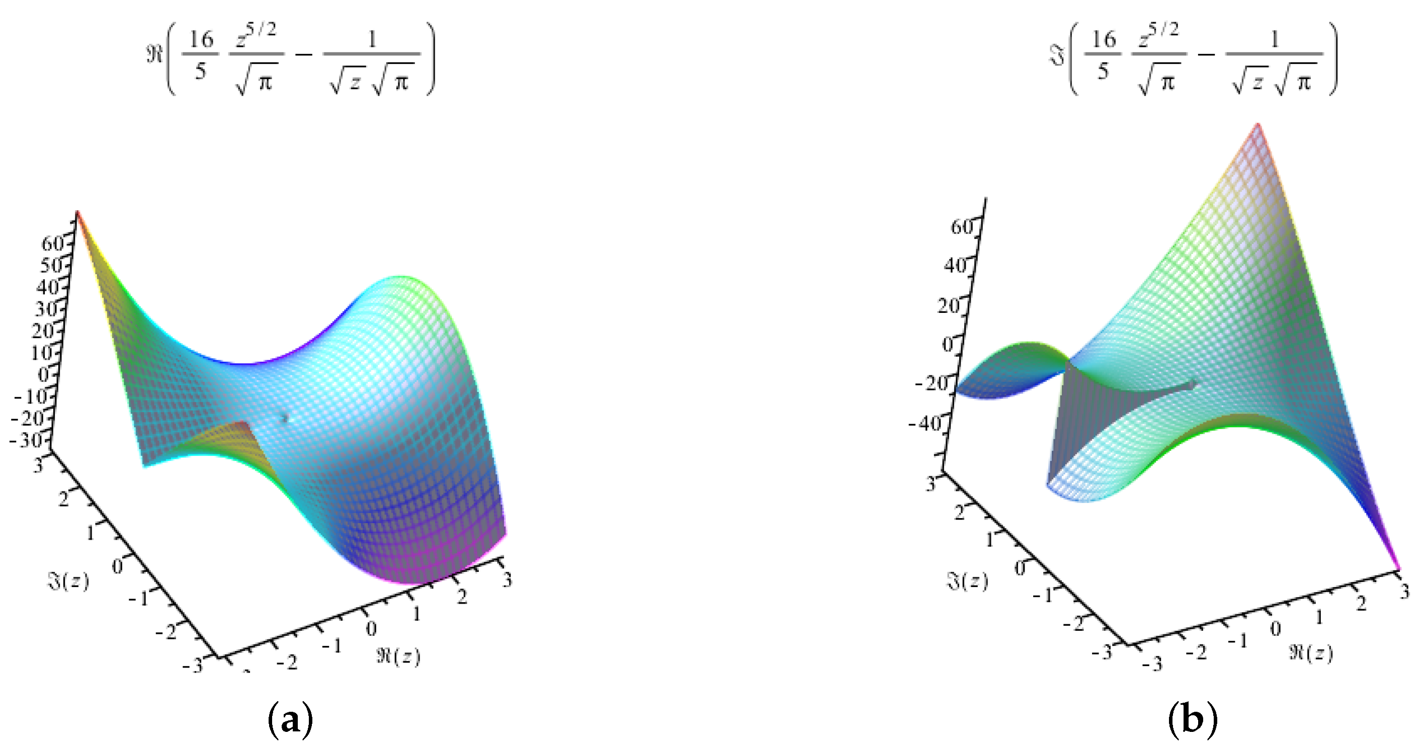
where $c=constant$. It is easy to see that $D_C^{\alpha }p\left(z\right)=D_{RL}^{\alpha }p\left(z\right)$ if and only if p has the constant term equal to zero. Equation (13) is well-defined because the branch cuts procedure remove the multi-valuedness in it. The branch cuts procedure has been implemented in many Computer Algebra Systems (CAS) (Maple and Matlab) and programming languages (Python and Java). For example, by using FunctionAdvisor tool in Maple [26], one can check the branch cut line and visualise real and imaginary parts of $D_{RL}^{1/2}(z^3-1)$. As one can see in Figure 1, the plots are continuous functions excluding the cut line, $\{z\in \mathbb{C}:Im(z)=0\wedge Re(z)<0\}$, along which the imaginary part of the plot has the jump.

Some general results with the detailed proofs concerning derivatives of analytic functions can be found in [18,27,28]. In [29,30], many new properties of fractional derivatives together with directional fractional derivatives are presented.

3. The Newton Method with Fractional Derivatives

Let us denote any complex polynomial by p. The well-known Newton’s method is defined as

$$z_{k+1}=z_k-\frac{p\left(z_k\right)}{p^{{}^{\prime }}\left(z_k\right)},k=0,1,2,\dots ,$$

(16)

with a starting point $z_0\in \mathbb{C}$. Equation (16) can be used to solve equation $p\left(z\right)=0$ in both real and complex domains.

By replacing the classical first-order derivative $p^{{}^{\prime }}\left(z\right)$ in Equation (16) by the Riemann–Liouville or the Caputo derivative of fractional order $\alpha$, both denoted as $D^{\alpha }p\left(z\right)$, we get

$$z_{k+1}=z_k-\frac{p\left(z_k\right)}{D^{\alpha }p\left(z_k\right)},k=0,1,2,\dots ,$$

(17)

with a starting point $z_0\in \mathbb{C}$. Equation (17) can be used to solve equation $p\left(z\right)=0$ in both the real and the complex domains. Further, Equation (17) for the RL derivative is called the fractional RL-Newton method and for the C derivative as the fractional C-Newton method.

At the beginning, we assumed that p is a complex polynomial. Because polynomials in the complex plane are very regular functions, as in the real case, thus the convergence properties of the fractional Newton’s method follow directly from the calculations presented by Brambila-Paz et al. in [12]. All these calculations are valid in our case for both $RL$ and C derivatives. The problem that appears is multivaluedness, which can be fixed by the branch cut method. Observe that the right hand-side of Equation (17) can be treated as an iteration function $\Phi$:

$$\Phi (z,\alpha )=z-\frac{p\left(z\right)}{D^{\alpha }p\left(z\right)}$$

(18)

with $\alpha$ as a parameter. When $\Phi$ is regular enough, the first and the second derivatives can be calculated and Taylor’s series expansion of the function $\Phi$ around a zero $\xi$ of p can be performed. If $\Phi$ is not regular enough, then some regularisation with the use of integral operator is required and Taylor’s series expansion is obtained for regularised $\Phi$. Then, similar to in [12], the following conclusion can be formulated: the fractional Newton method in Equation (17) converges at least linearly when $\alpha \ne 1$ and at least quadratically when $\alpha =1$ for polynomials with zeros of multiplicity one.

4. Numerical Experiments

In this section, the results of graphical and numerical experiments are presented. The experiments were conduced for several polynomials by using the RL-Newton and the C-Newton methods with various values of parameter $\alpha \in (0,2)$.

The graphical examples are obtained through the methods of polynomiography. We selected polynomiographs obtained with two colouring methods, namely basins of attraction and colouring with respect to the number of iterations (the so-called iteration colouring). The general algorithm for the generation of polynomiograph is presented in Algorithm 1. In the algorithm, the $convergenceTest(z_{k+1},z_k,\epsilon )$ returns $TRUE$ if the method has converged to the root, and $FALSE$ otherwise. The two most widely used convergence tests are the following:

$$\begin{array}{c}\left|p\right(z_{k+1}\left)\right|<\epsilon ,\end{array}$$

(19)

$$\begin{array}{c}|z_{k+1}-z_k|<\epsilon .\end{array}$$

(20)

Algorithm 1: Polynomiograph generation.

The last step of the algorithm colours the point according to the selected colouring method. In the basins of attraction colouring, each root gets a distinct colour (other than black). Next, if the number of performed iterations is less than M, then for the obtained approximation $z_{k+1}$ the algorithm searches for the closest root—by using the modulus metric—and colours the starting point with the colour of the root. If the number of performed iterations is equal to M, then the starting point gets the black colour. In iteration colouring, the starting point is coloured by mapping the number of performed iterations on the colour in the colour map.

In the numerical experiments, we used three different measures to compare the use of Riemann–Liouville and Caputo fractional derivatives: average number of iterations [9], convergence area index [6], and generation time [10]. All measures were calculated from the polynomiographs.

To compute the first measure, namely the average number of iterations (ANI), we used polynomiograph P coloured with the iteration colouring. In this type of polynomiograph, each point is coloured according to the number of iterations needed to find a root. We used a linear mapping for this aim, i.e., each iteration was linearly mapped onto a colour in a given colour map. The value of ANI was computed as the mean number of iterations in P.

Similar to ANI, the convergence area index (CAI) was computed from polynomiograph P coloured by using the iteration colouring. First, we counted the number of converging points $N_c$, i.e., points in P whose number of iterations is less than the maximum number of iterations. Then, the value of CAI was computed in the following way

$$CAI=\frac{N_c}{N},$$

(21)

where N is the total number of points in P. CAI gives us information about the percentage of the polynomiograph’s area that has converged to roots. It takes values in $[0,1]$, where 0 means that no point has converged, and 1 means that all points have converged.

The last measure is the time of generation of the polynomiograph. This measure is very similar to ANI, but it gives us information about the actual time of computations. ANI does not take into account the cost of computations in a single iteration. Thus, two methods with the same value of ANI can have different generation times due to different computational complexities in a single iteration.

Following the authors of [7,8], we used the same polynomials in the experiments, namely

$$\begin{array}{c}{p}_n\left(z\right)=z^n-1\mathrm{for}n=2,3,4,\\ p_6\left(z\right)=z^6-\frac{1}{2}{z}^5+\frac{11}{4}(1+i)z^4-\frac{1}{4}(19+3i)z^3+\frac{1}{4}(11+5i)z^2-\frac{1}{4}(11+i)z+\frac{3}{2}-3i.\end{array}$$

The sets of roots for these polynomials are the following:

• $\{-1,1\}$ for $p_2$,
• $\{-\frac{1}{2}-\frac{\sqrt{3}}{2}i,-\frac{1}{2}+\frac{\sqrt{3}}{2}i,1\}$ for $p_3$,
• $\{-1,1,-i,i\}$ for $p_4$,
• $\{1,1-i,-1+2i,-\frac{1}{2}(1+i),-\frac{3}{2}i,i\}$ for $p_6$.

For polynomials $p_2$, $p_3$ and $p_4$, we used the area $[-2,2]\times [-2,2]$ for the polynomiographs, whereas for, $p_6$, we changed the area to $[-3,3]\times [-3,3]$ to cover all polynomial roots. The other parameters used for the generation of polynomiographs were the following: resolution $600\times 600$ pixels, $M=40$, $\epsilon =0.001$, and the convergence test in Equation (). The colour map used for the colouring of iterations is presented in Figure 2. The values of $\alpha$ were changed with the step $0.01$.

All experiments were performed on a computer with the following specifications: Intel Core i5-4570 processor, 16 GB RAM, Windows 10 (64-bit). The software for polynomiograph’s generation was implemented in Processing, a programming language based on Java.

4.1. The Results of Experiments

For clear exposition of the obtained results, the polynomials are presented in the following sequence (depending on $\alpha$-order in $(0,2)$): basins of attraction for $RL$-Newton and C-Newton methods, iteration coloured polynomiographs for $RL$-Newton and C-Newton methods and plots of ANI, CAI and the generation time for the $RL$-Newton and C-Newton methods. Moreover, for each polynomial, we show polynomiographs and values of ANI, CAI and the generation time for the classical Newton’s method (Equation (16)). These results are used as the reference for the results obtained by using the methods with fractional derivatives.

4.1.1. Polynomial $p_2$

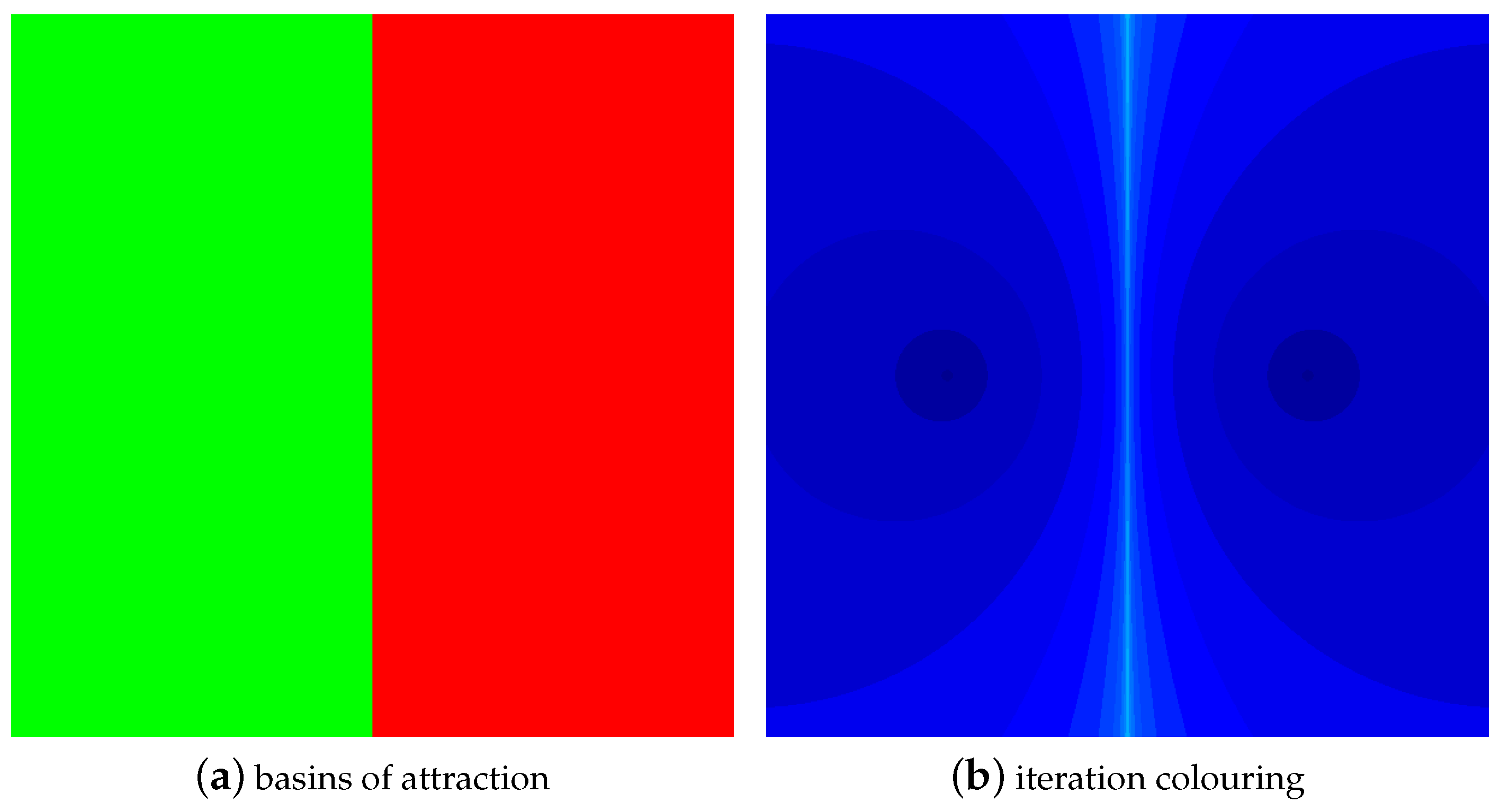
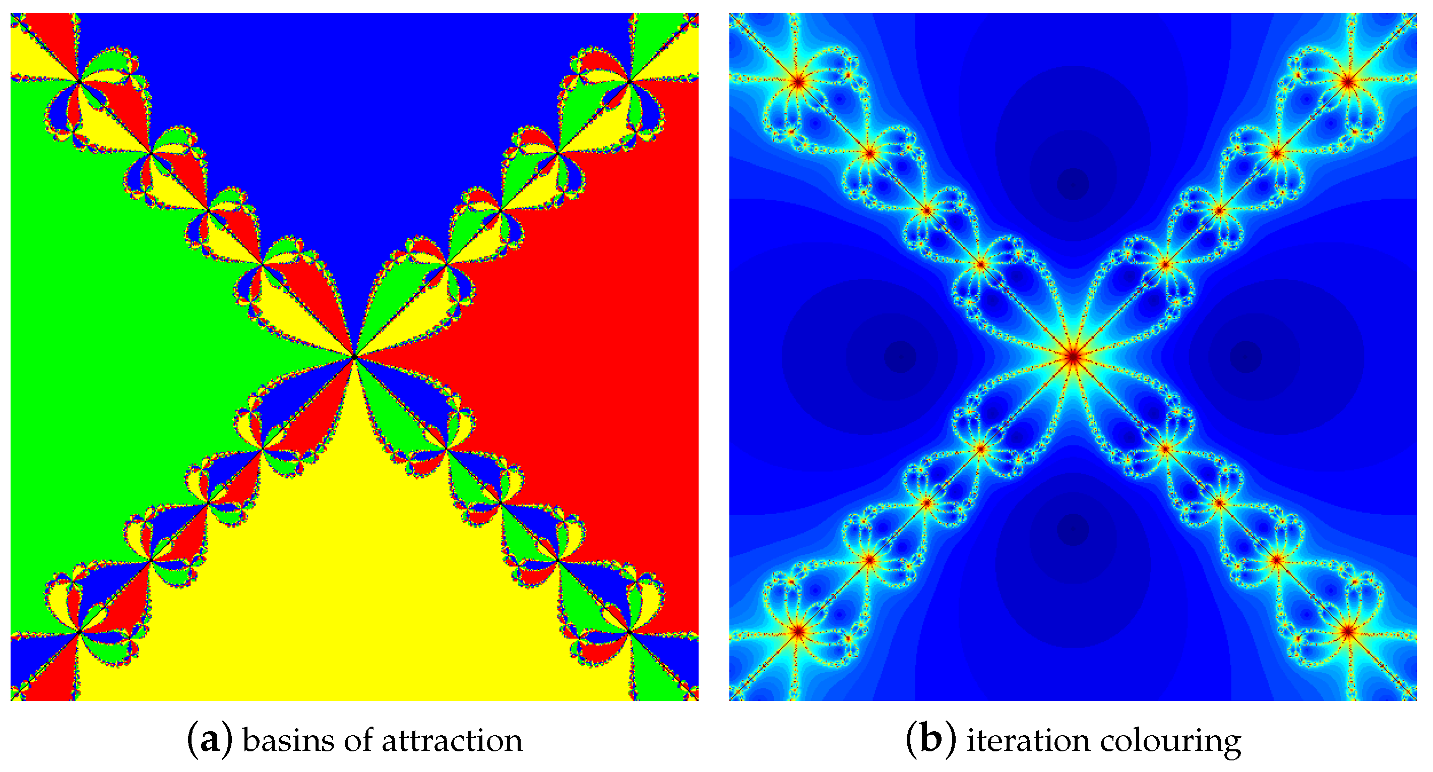
Polynomiographs obtained by the classical Newton’s method are presented in Figure 3. The values of ANI, CAI and the generation time are equal to $3.406$, $1.0$ and $0.366$ s, respectively.

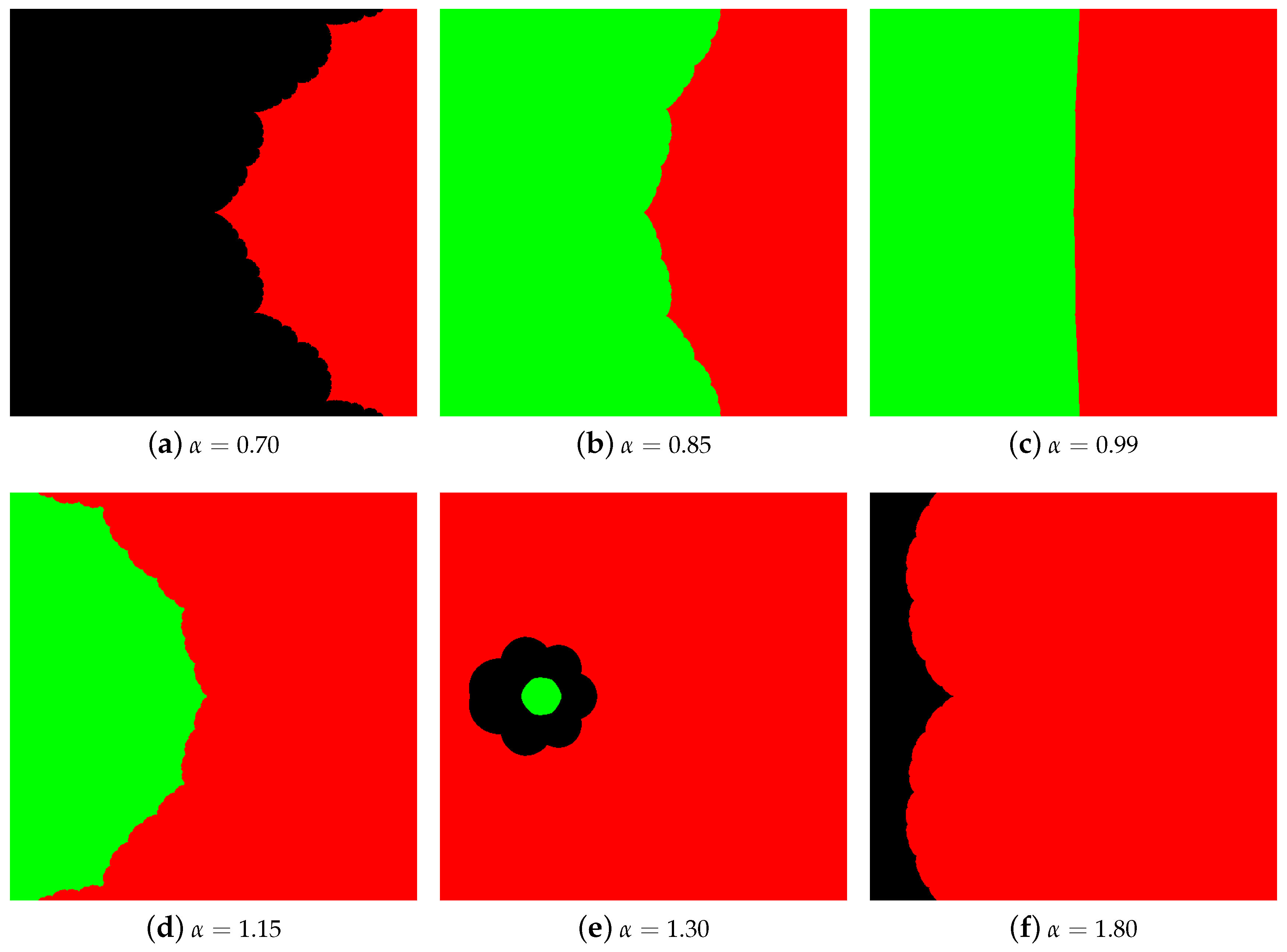
The basins of attraction for the RL-Newton and C-Newton methods are presented in Figure 4 and Figure 5, respectively. The presented basins were generated for various values of $\alpha$: (a) $0.70$; (b) $0.85$; (c) $0.99$; (d) $1.15$; (e) $1.30$; and (f) $1.80$. By looking at the basins of attraction for $\alpha$ close to 1, i.e. $\alpha =0.99$ (Figure 4c and Figure 5c), we see that, compared to the classical Newton’s method (Figure 3a), the boundaries between the basins are changing. In the case of the classical Newton’s method, this boundary is a straight line. For the RL-Newton method, the boundary bends lightly and some smaller areas are isolating along it, and, for the C-Newton method, the boundary undergo only the bending process. When the value of $\alpha$ is decreasing we see that the boundary for both methods is bending further (Figure 4b and Figure 5b), and, in the case of the RL-Newton method, the isolated areas are enlarging. With a further decreasing of $\alpha$, the methods stop converging to one of the roots and even stop converging at all (black areas in the polynomiographs). In the case of increasing $\alpha$ above 1, we also see boundary bending, but it is directed in the opposite direction relatively to the direction for $\alpha <1$ (see Figure 4d and Figure 5d). When one increases the value of $\alpha$, the basin of one of the roots is shrinking and points for which the methods do not converge to any root are appearing (Figure 4e and Figure 5e). With the further increase of $\alpha$, we see a continued shrinking of one of the basins and worsening of the convergence for the RL-Newton method (Figure 4f), and, in the case of the C-Newton method, the method converges to only one of the roots or it does not converge at all (Figure 5f).

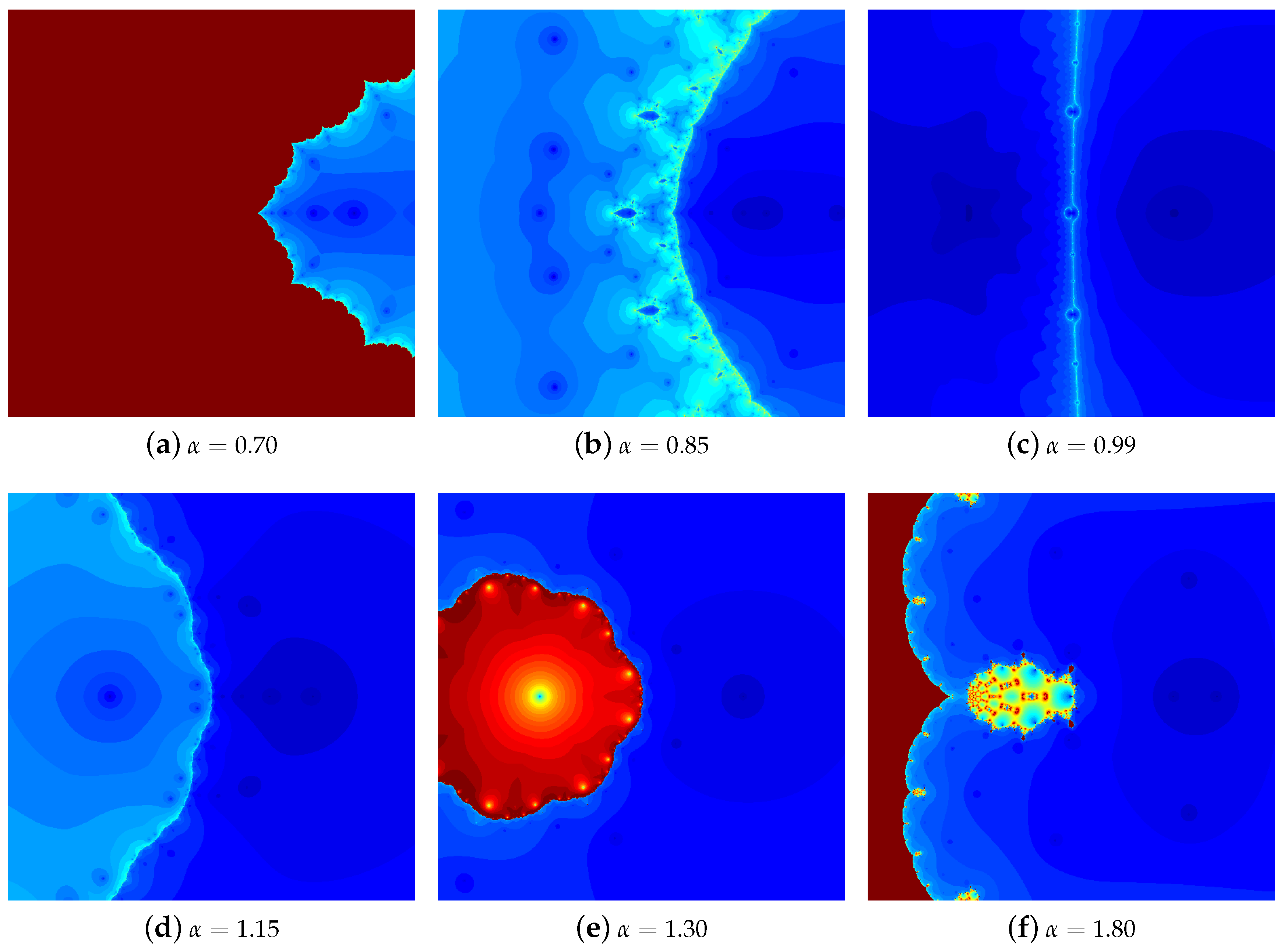
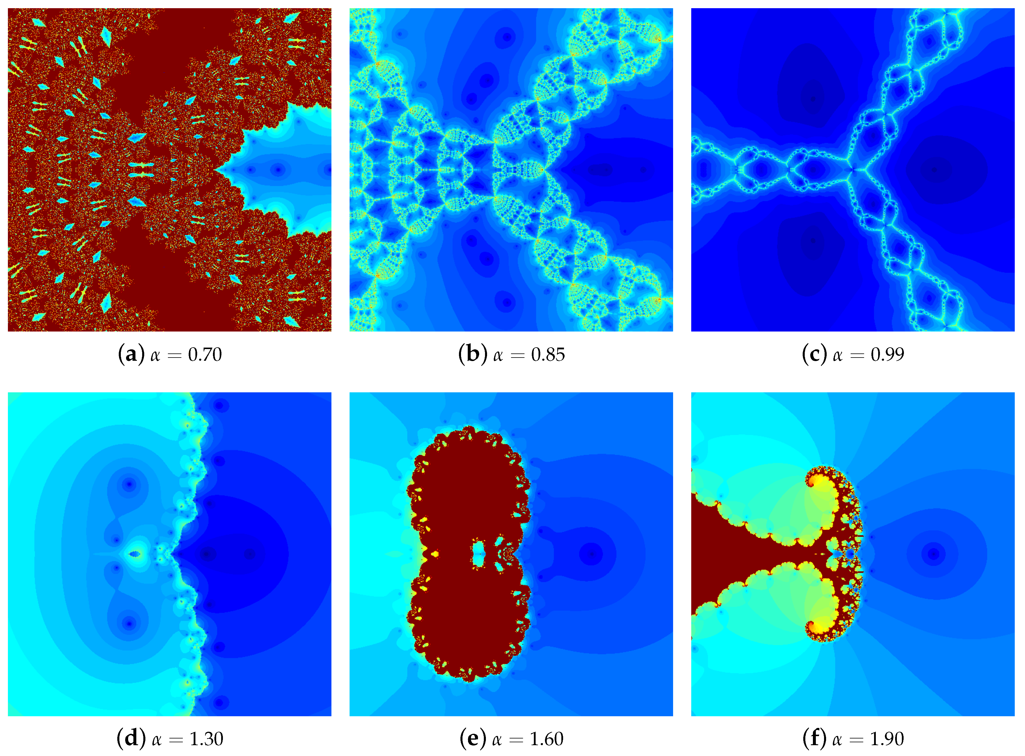
The polynomiographs obtained with the iteration colouring for the same values of $\alpha$ as for the basins of attraction are presented in Figure 6 and Figure 7. For $\alpha$ close to 1 (Figure 6c and Figure 7c), the area with a light blue colour in the central part bends in comparison to the classical Newton’s method (Figure 3b). The bending is similar to the one visible for the basins of attraction. In the other parts of the polynomiograph, the shape of the areas corresponding to the same number of iterations is changing. With the shape change, the dynamics of the methods also changes. When one decreases the value of $\alpha$, one can observe a similar behaviour as for the basins of attractions, i.e., further bending of the central part (Figure 6b and Figure 7b). Moreover, the dynamics of both methods is increasing, creating very interesting patterns. We can also observe that, to the left of the bent boundary, the number of iterations needed for finding the root is increasing in a significant way in comparison to the right area. After further decreasing of $\alpha$, the areas where methods stop to converge to the roots are appearing (red colour in Figure 6a and Figure 7a). In the other areas, we see further change of the regions corresponding to the same number of iterations and the increase of the number of iterations performed by the methods. Increasing the value of $\alpha$ above 1 causes the bending of the central part of the polynomiograph (Figure 6d and Figure 7d), which is similar to the bending that we have seen for the basins of attraction. We also see that the number of iterations is increasing, which is especially visible to the left from the bent part. With the further increase of $\alpha$ (Figure 6e and Figure 7e), we see that points for which the methods need large number of iterations or they do not converge to any root appear. Simultaneously, the dynamics of the methods is decreasing. For $\alpha$ close to 2 (Figure 6f and Figure 7f), we can observe further increase of the number of points for which the methods do not converge. In the case of the RL-Newton method, an area with an increased dynamics appears, and, for the C-Newton method, the dynamics is decreasing.

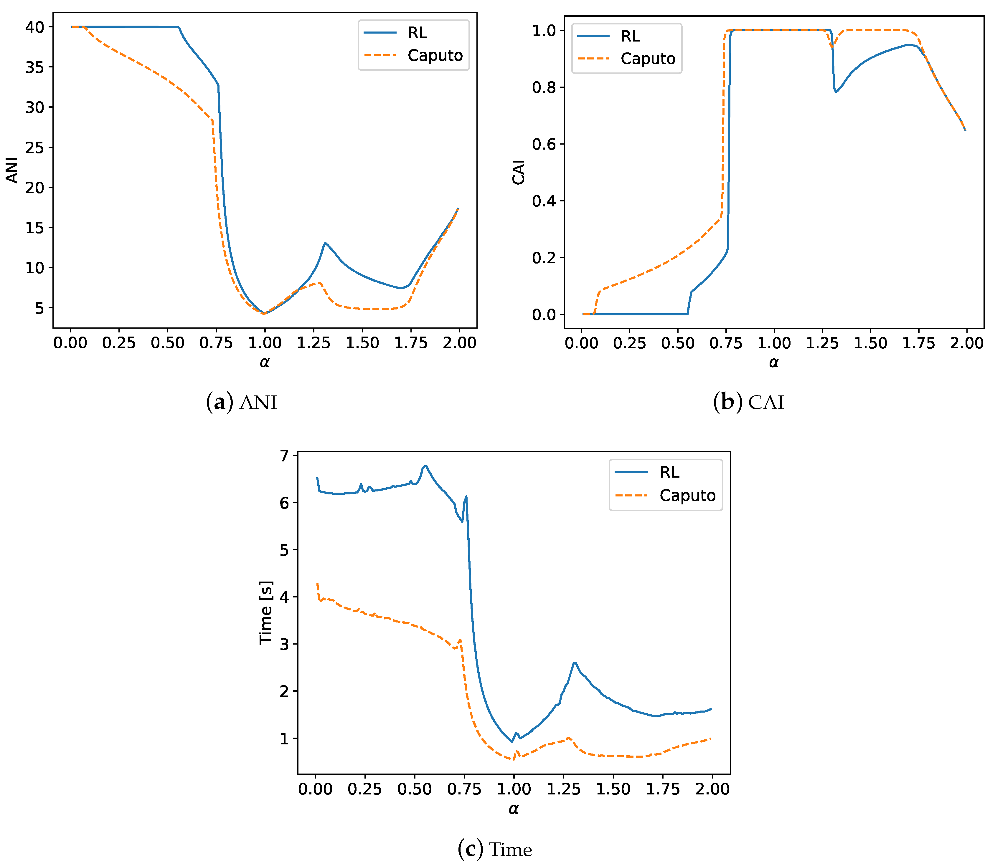
The numerical results obtained for $p_2$ are presented in Figure 8. In Figure 8a, we see the results for ANI. In the case of both methods, the lowest values of ANI are obtained close to $\alpha =1$. The minimal value of ANI equals to $4.310$ for the RL-Newton method and $4.241$ for the C-Newton method. Both are attained at $\alpha =0.99$. Comparing these results to the classical Newton’s method ($3.406$), we see that the average number of iterations in the methods with the fractional derivatives is larger. Looking at the plots for the both methods, we can observe that the decreasing of $\alpha$ below 1 causes that the ANI is increasing very fast (we can also observe this in Figure 6 and Figure 7 by the change of shades of blue, to lighter shades, and by the appearance of the red colour). For the RL-Newton method for $\alpha <0.55$, we see that the method needs 40 iterations on average, thus it is not convergent at all. In the case of the C-Newton method, we can observe a similar effect, but for a much lower value of $\alpha$, namely for $\alpha <0.04$. When we increase the value of $\alpha$ above 1, we also see the growth of the value of ANI, but not as significant as for $\alpha <1$. Irrespective of the $\alpha$ value, the C-Newton method obtains lower values of ANI. The results obtained for CAI are presented in Figure 8b. Both methods obtained the maximal value of CAI, equal to $1.0$, in the intervals $(0.79,1.29)$ and $(0.77,1.25)\cup (1.38,1.68)$ for the RL-Newton and C-Newton methods, respectively. Therefore, both methods have obtained in a wide range the identical result as the classical Newton’s method. Outside of these intervals we can observe decrease of CAI value, wherein for $\alpha <0.77$ for the RL-Newton method and for $\alpha <0.74$ for the C-Newton method the decrease is rapid and the methods are reaching value equal to $0.0$ for $\alpha <0.55$ for the RL-Newton method and for $\alpha <0.06$ for the C-Newton method. Again, irrespective of the $\alpha$ value, the C-Newton method obtains values of CAI larger than the RL-Newton method. In Figure 8c, we see plots with the times of generation of the polynomiographs. For both methods, we can observe a very similar behaviour to the one obtained for ANI. Both methods obtained the shortest times close to $\alpha =1$, namely $0.924$ s at $\alpha =0.99$ for the RL-Newton method and $0.522$ s at $\alpha =1.0$ for the C-Newton method. The minimal values for both methods are higher than for the classical Newton’s method ($0.366$ s). By changing the values of $\alpha$ we see that the generation times are increasing. For $\alpha <1$, the growth is significant, obtaining the maximal value of time equal to $6.773$ s (at $\alpha =0.56$) for the RL-Newton method and $4.284$ s (at $\alpha =0.01$) for the C-Newton method. Unlike in the case of ANI, the differences between the RL-Newton and C-Newton methods are more visible, in favour of the C-Newton method. In the case of $\alpha >1$, the increase is much lower and the methods obtain the maximal value of $2.598$ s (at $\alpha =1.31$) for the RL-Newton method and $1.011$ s (at $\alpha =1.27$) for the C-Newton method. In addition, in this case, the C-Newton method obtains shorter times.

4.1.2. Polynomial $p_3$

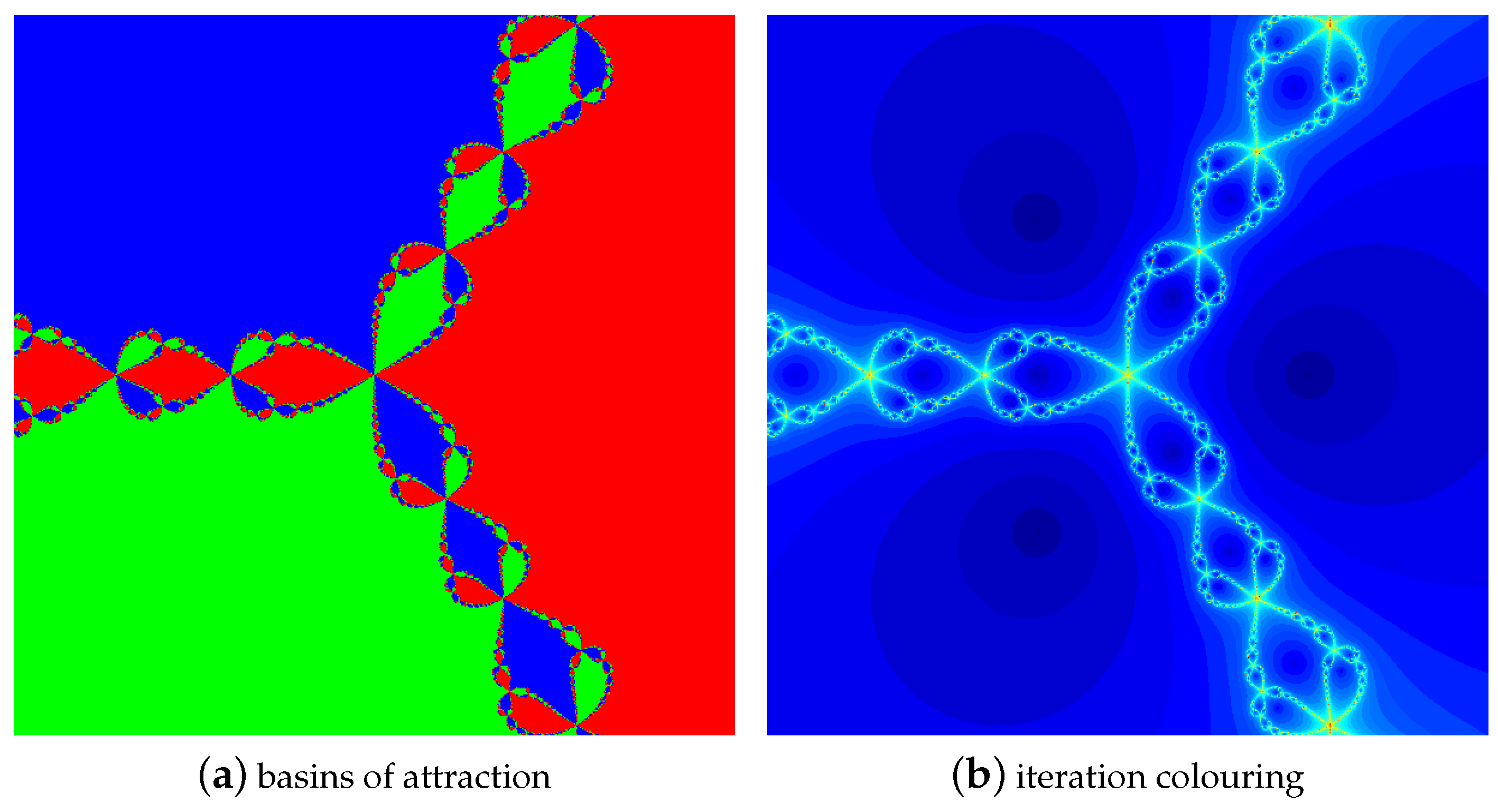
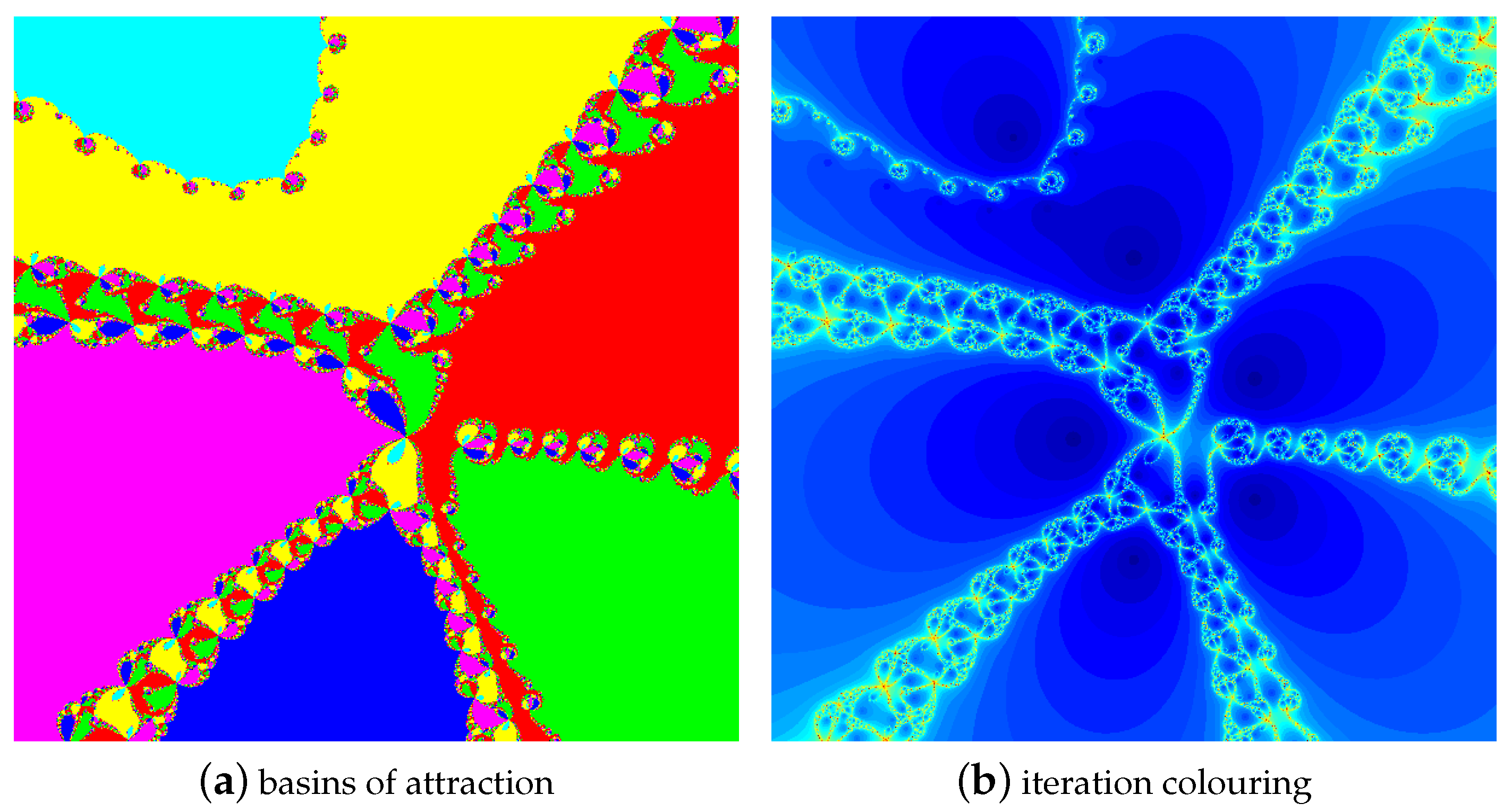
Polynomiographs of $p_3$ obtained by the classical Newton’s method are presented in Figure 9. The values of ANI, CAI and the generation time are equal to $5.056$, $1.0$ and $0.611$ s, respectively. Both polynomiographs are symmetric. They present three basins of attraction in Figure 9a and the three roots of unity are clearly visible as dark blue circles in Figure 9b. Boundaries among three areas of the polynomiographs have a complicated fractal structure resembling the shape of braids.

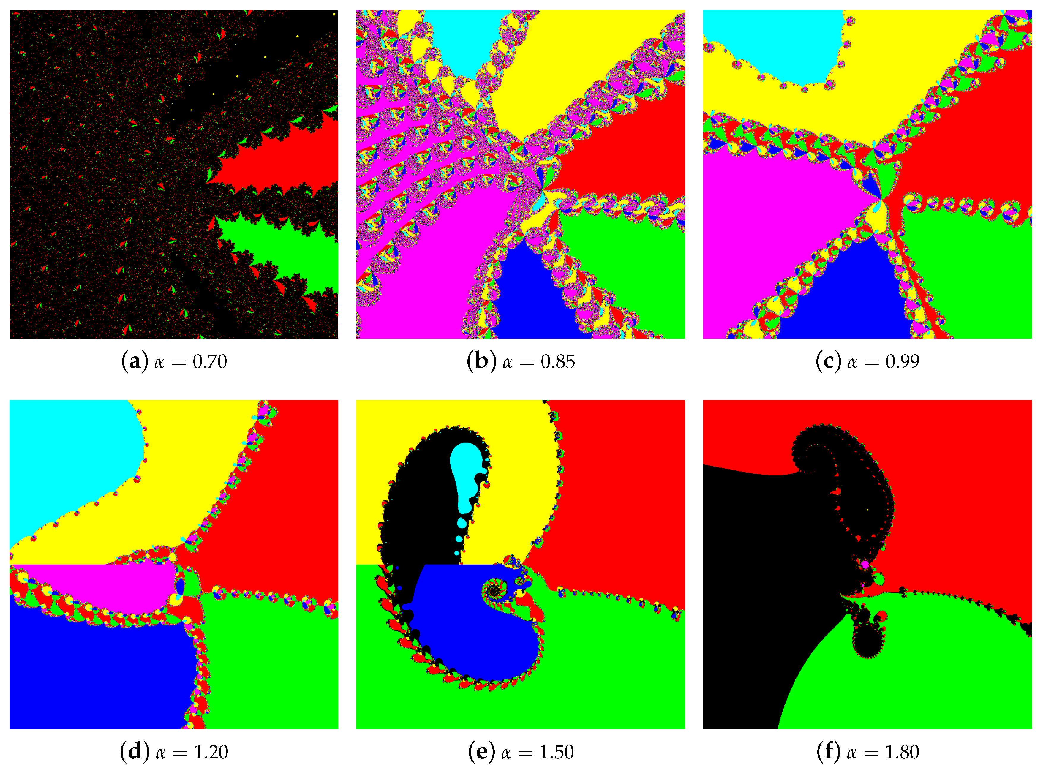
Figure 10 and Figure 11 show basins of attraction for the RL-Newton and C-Newton methods, respectively, for fixed $\alpha$ values: (a) $0.70$; (b) $0.85$; (c) $0.99$ (d) $1.30$; (e) $1,60$; and (f) $1.90$. For $\alpha$ of $0.70$, $1.60$, and $1.90$ (RL-Newton method) and for $\alpha$ of $1.60$ and $1.90$ (C-Newton method), only one red basin of real root 1 exists, covered by black visible areas of non-convergence (larger for RL-Newton method), as shown in Figure 10a,e,f and Figure 11e,f, respectively. Around $\alpha =0.85$ (RL-Newton method, Figure 10b) and for $\alpha =0.70$ (C-Newton method, Figure 11a), besides the basin of the real root 1, additionally two basins of conjugate $p_3$ roots appear. The boundary between them has the form of a wide bunch of braids covered, in the case of the C-Newton method, by small black regularly distributed areas of non-convergence gradually disappearing for $\alpha$ slightly greater than $0.70$. For values of $\alpha$ close to 1, basins for both fractional methods are very similar as for the classical Newton method (Figure 9a). In Figure 10d and Figure 11d, one can see that, for $\alpha$ around $1.30$, for the both fractional methods, the boundary between conjugate $p_3$ roots is a straight segment, whereas, on the other boundaries, small artefacts are visible, larger in the case of the C-Newton method.

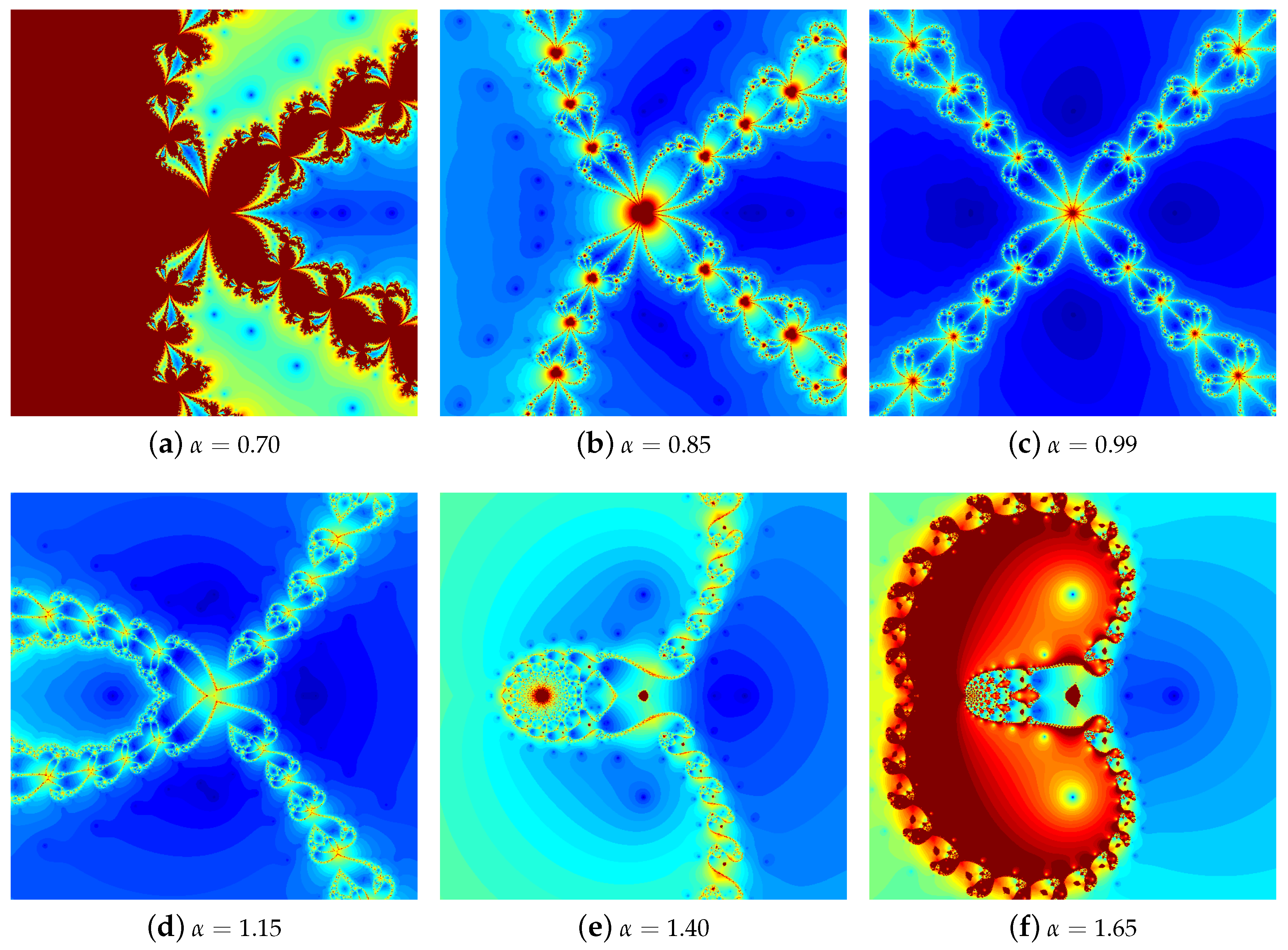
Iteration colouring polynomiographs for $p_3$ presented in Figure 12 and Figure 13 reveal strong dependence of their images on the $\alpha$ order. Generally speaking, polynomiographs generated by both fractional methods are asymmetric apart from the case of $\alpha$ close to 1 corresponding to the classical Newton’s method. More blue in the images means higher speed of convergence, whereas yellowish-brownish means slow convergence. Dark blue areas show roots of $p_3$, well visible if $\alpha$ is close to 1. Colouring stresses the dynamics of the methods. With $\alpha$ increasing in the range $(0.70,1.90)$ for RL-Newton method, one can observe in Figure 12 the following sequence of images: (a) very small area of convergence; (b,c) three distinct areas with shrinking braids among them; (d) vanishing boundary among conjugate roots of $p_3$; and (e–f) enlarging areas of non-convergence with visible real root. The sequence of images for C-Newton method (Figure 13) starts from highly dynamical in Figure 13a and continues in Figure 13b–f similarly to those for RL-Newton method, but looking more subtle.

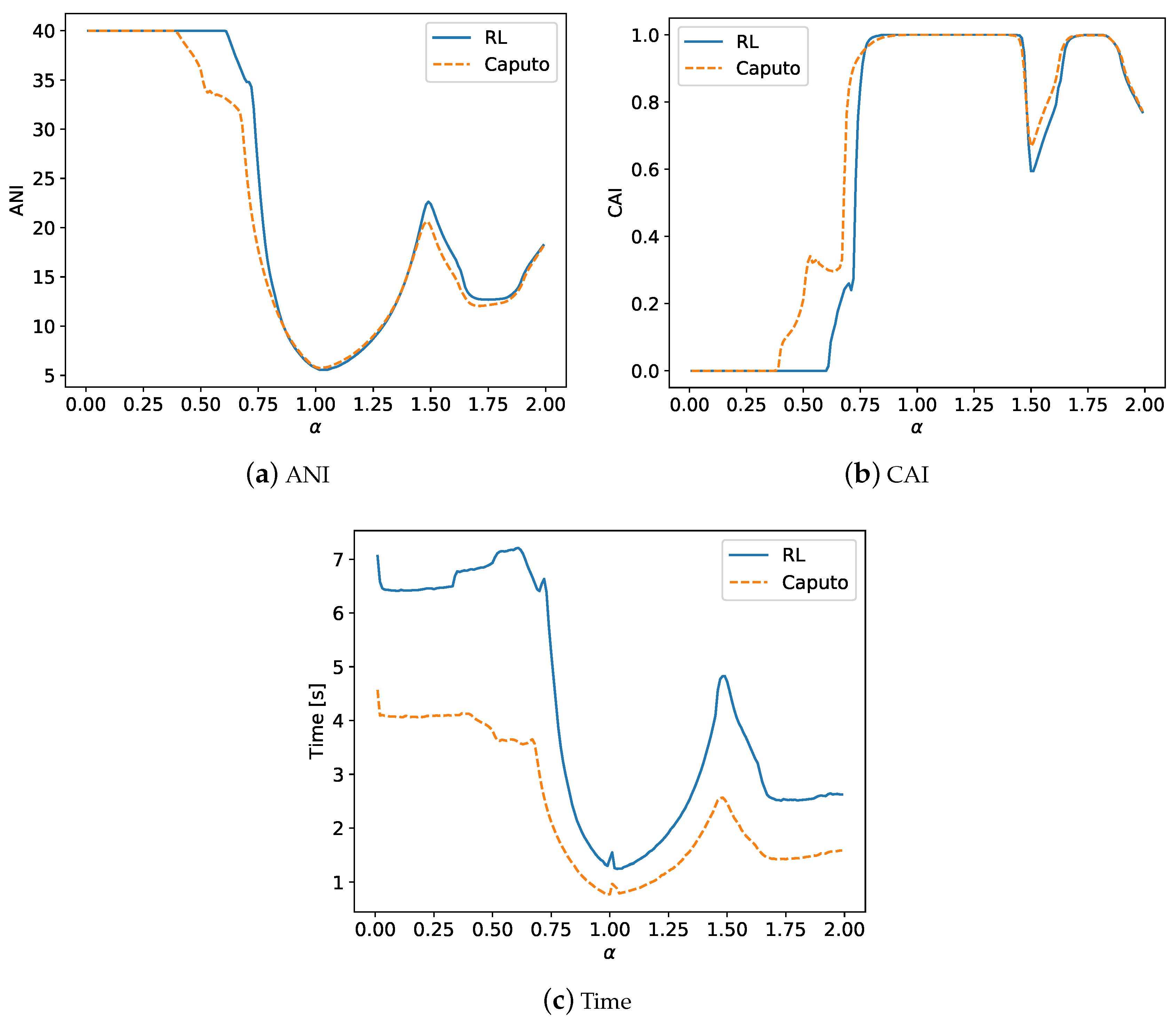
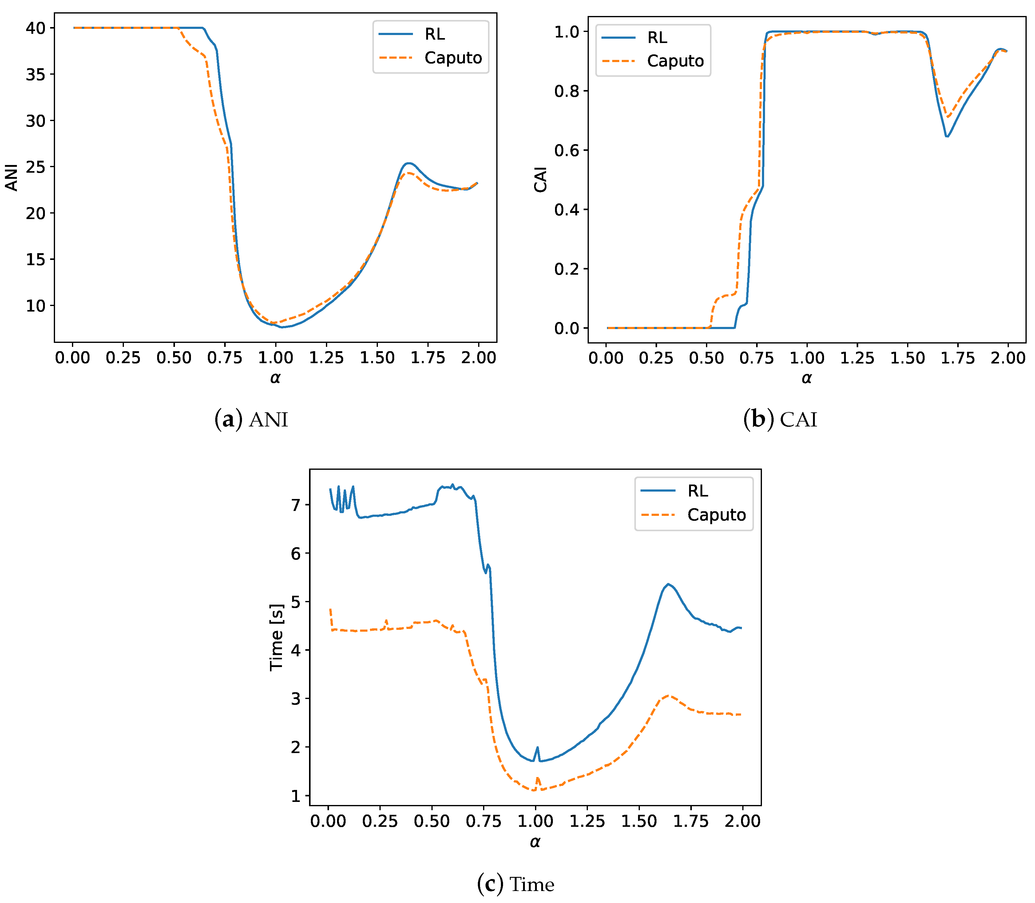
From ANI and CAI plots presented in Figure 14a,b, respectively, one can see that, for $\alpha$ in the range $(0.75,2)$, in both plots, the runs for both methods are almost identical. That means that both fractional methods behave similarly. In Figure 14c, it is seen that the time of generation is shorter for the C-Newton method. The minimal time of generation of polynomiographs is for $\alpha$ close to 1. More detailed analysis of numerical data shows that, for $\alpha \in (0,0.6)$ (RL-Newton method) and $\alpha \in (0,0.36)$ (C-Newton method), the average number of iterations is maximal (40). That means that neither method is convergent. Starting from $\alpha =0.36$ for the RL-Newton method and $\alpha =0.36$ for the C-Newton method, the ANI measure quickly decreases and attains its minimal value $5.551$ for $\alpha =1.04$ and $5.745$ for $\alpha =1.02$ for the RL-Newton and the C-Newton method, respectively. If $\alpha$ increases further for both fractional methods, the increase of ANI measure is observed until achieving local maximum equal to 20 iterations at $\alpha =1.51$ (RL-Newton method) and $\alpha =1.48$ (C-Newton method). From CAI plots (Figure 14b), one can see that, for $\alpha <0.36$ (RL-Newton method) and $\alpha <0.6$ (C-Newton method), neither fractional method is convergent (CAI is zero). Further one can observe that for $\alpha$ in $(0.85,1.42)\cup (1.72,1.81)$ almost all points are convergent in both fractional methods. In Figure 14c, presenting the generation times of polynomiographs, it is visible that, for $\alpha \in (0.75,1.75)$, the generation time plots, in general, are similar to ANI plots. For $\alpha =0.99$, the times of generation attain their minima equal to $1.302$ s (RL-Newton method) and $0.769$ s (C-Newton method). It is interesting that ANI and the generation time attain local maximum for $\alpha$ equal approximately $1.5$, whereas CAI attains its local minimum for both fractional methods.

4.1.3. Polynomial $p_4$

The polynomiographs obtained by the classical Newton’s method are presented in Figure 15. The values of ANI, CAI and the generation time are equal to $7.440$, $0.994$ and $0.919$ s, respectively.

The basins of attraction for polynomial $p_4$ are presented in Figure 16 and Figure 17 for RL-Newton and C-Newton methods, respectively, for $\alpha \in \{0.70,0.85,0.99,1.15,$$1.40,1.65\}$. As one can see for $\alpha =0.99$, the general shapes of the basins are quite predictable in comparison to $p_3$ for both methods. The differences lie only in details. For $p_4$, there are four braids and the polynomiographs are also symmetric. For the other values of $\alpha$, the symmetry is broken bending the braids from the left or the right side depending on whether $\alpha$ is decreased or increased.

In Figure 18 and Figure 19, there are shown polynomiographs for RL-Newton and C-Newton methods, respectively. As one can see, their general shapes are similar as in the case of basins of attraction. Similarly, as in the case of the above presented polynomials $p_2$ and $p_3$, dark blue colour represents the roots of $p_4$. They are well visible for $\alpha =0.99$ (Figure 18c and Figure 19c). Next, the smaller or larger is the value of $\alpha$, the lesser is the dynamic of convergence (visible as more brown colour).

Figure 20 presents plots of ANI, CAI and the generation time for $p_4$. As one can see, for both methods, RL-Newton and C-Newton, for the small value of $\alpha$, the average number of iterations is maximal (Figure 20a). This means that, for $\alpha <0.64$ for the RL-Newton method and for $\alpha <0.5$ for the C-Newton method, these methods have not converged. Starting from $\alpha =0.65$, ANI intensively decreases for both methods and achieves its minimum for $\alpha =1.03$ for the RL-Newton method and $\alpha =0.99$ for the C-Newton method. These minima are equal to $7.638$ for the RL-Newton method and $8.106$ for the C-Newton method. For $\alpha >1.03$, ANI increases slowly, achieving the maximum at about 24–25 iterations. As one can expect, by analysing the plot of CAI (Figure 20b), for $\alpha <0.5$ and for $\alpha <0.65$, the number of converging points for the RL-Newton and the C-Newton methods, respectively, equal zero. For $\alpha$ from $(0.83,0.97)\cup (1.01,1.28)$, all points converge in RL-Newton method and nearly all points (but not all) converge in C-Newton method. By analysing the last plot (Figure 20c), one can observe that the generation time for RL-Newton method has fluctuations for small values of $\alpha$. Both methods achieve their minimal times for $\alpha =1.03$ and $\alpha =0.99$ for RL-Newton and C-Newton methods, respectively. As in the case of the other polynomials, one can see that the C-Newton method is faster than the RL-Newton one. From all these plots, it is easily seen that at $\alpha =1.65$ in all plots there is maximum or minimum.

4.1.4. Polynomial $p_6$

The polynomiographs obtained by the classical Newton’s method are presented in Figure 21. The values of ANI, CAI and the generation time are equal to $7.984$, $1.0$ and $1.368$ s, respectively.

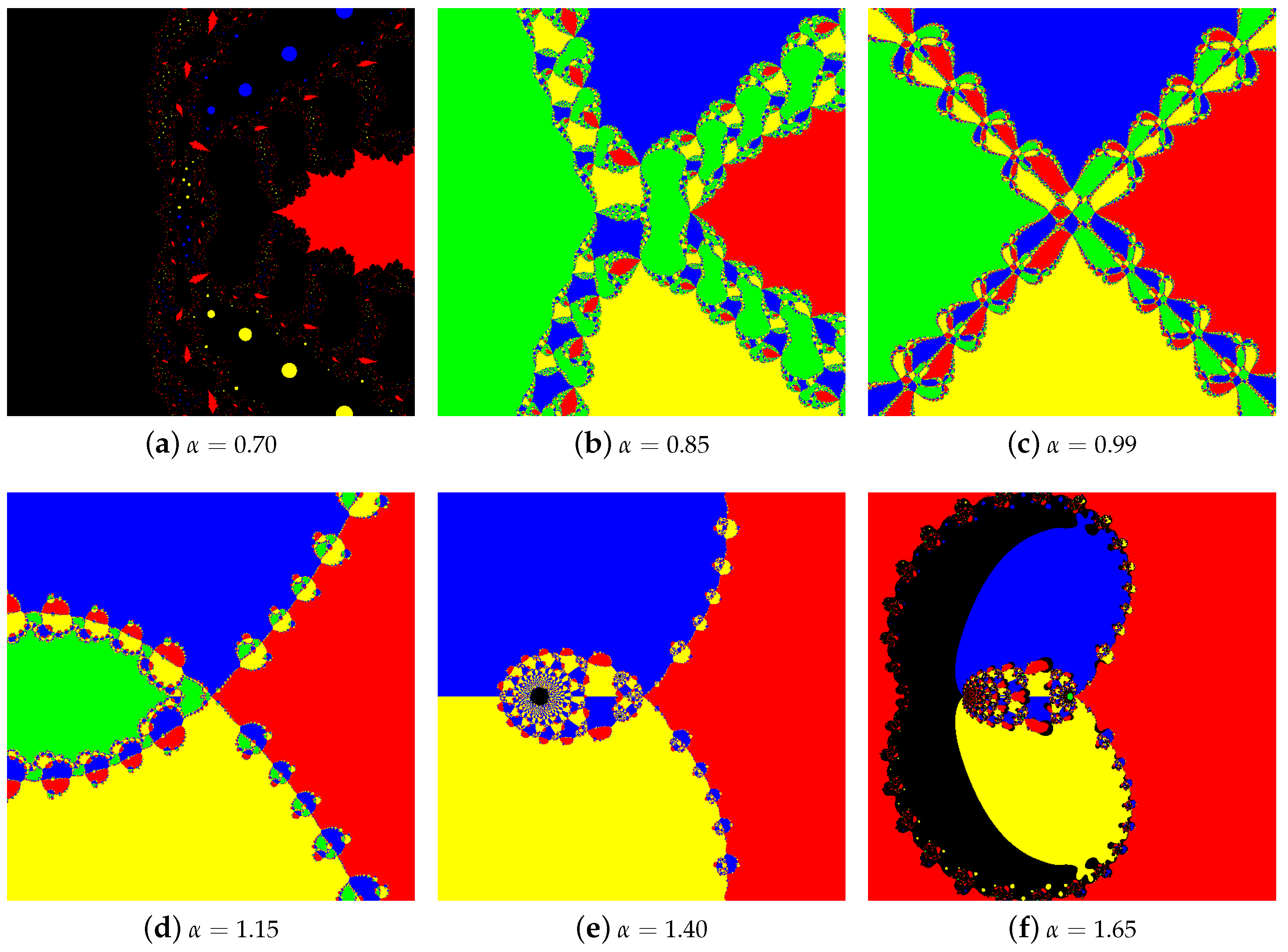
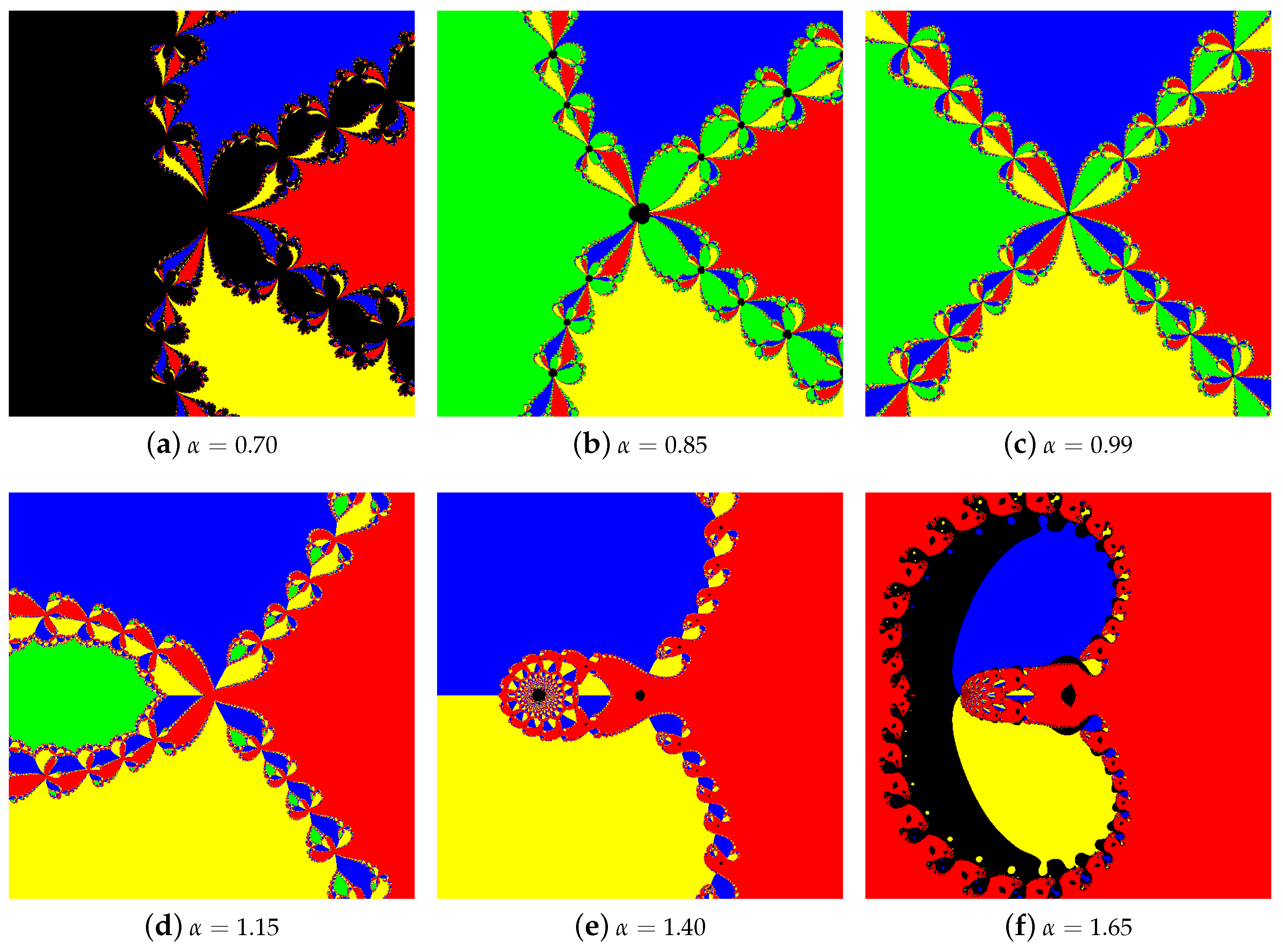
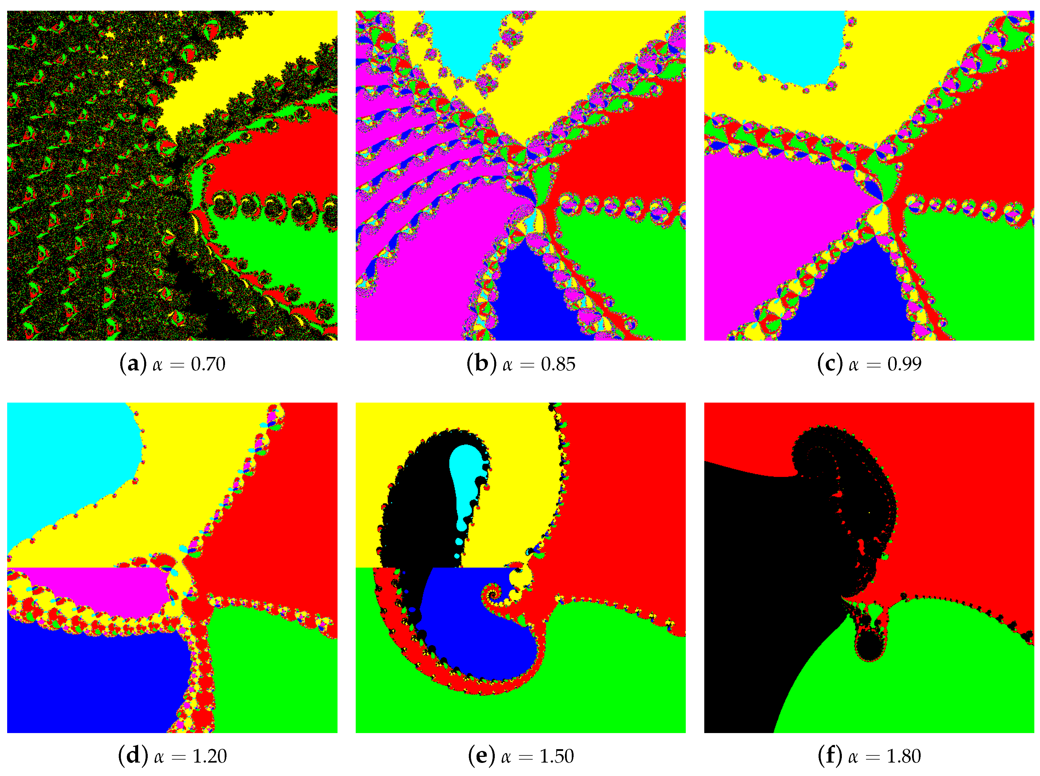
The basins of attraction for the RL-Newton and C-Newton methods are presented in Figure 22 and Figure 23, respectively. The presented basins were generated for various values of $\alpha$: (a) $0.70$; (b) $0.85$; (c) $0.99$; (d) $1.20$; (e) $1.50$; and (f) $1.80$. For $\alpha =0.99$ (Figure 22c and Figure 23c), by comparing the basins with the basins obtained with the classical Newton’s method, we see that the change of their shape is very small. The most noticeable change is visible in the braids on the left, i.e., they move a little bit away from the real axis. When the value of $\alpha$ is decreasing (Figure 22b and Figure 23b), we see that the lower-left braid is moving further away from the real axis, whereas the upper-left is splitting into many smaller braids. For the RL-Newton method, the splitting is more chaotic than for the C-Newton method. With a further decrease of the $\alpha$ order, the methods stop converging to some of the roots; we see only basins for three roots (red, green and yellow) out of six. In the case of the RL-Newton method, the yellow basins are very small compared to the C-Newton method. Moreover, many of the points in the considered area do not converge for either method (black colour in the polynomiographs). In the case of increasing $\alpha$ above 1, we see more interesting changes in the shape of the basins. The braids are getting smaller and, at the same time they, are bent (see Figure 22d and Figure 23d). For $\alpha =1.50$ (Figure 22e and Figure 23e), we can observe that the braids from the upper-left part of Figure 22c and Figure 23c are joining together and that some of the basins are shrinking. Moreover, we see that a spiral pattern appears near the centre. For high values of $\alpha$, i.e., $\alpha =1.80$ (Figure 22f and Figure 23f), we see that both fractional methods converge mostly to only two roots. For the other roots, the basins are very small or they disappear: the cyan basin is not present in either polynomiograph, whereas the blue and magenta basins disappear for the C-Newton method. Furthermore, the area in which the methods do not converge to any root increases, but not so much as in the case of $\alpha <1$.

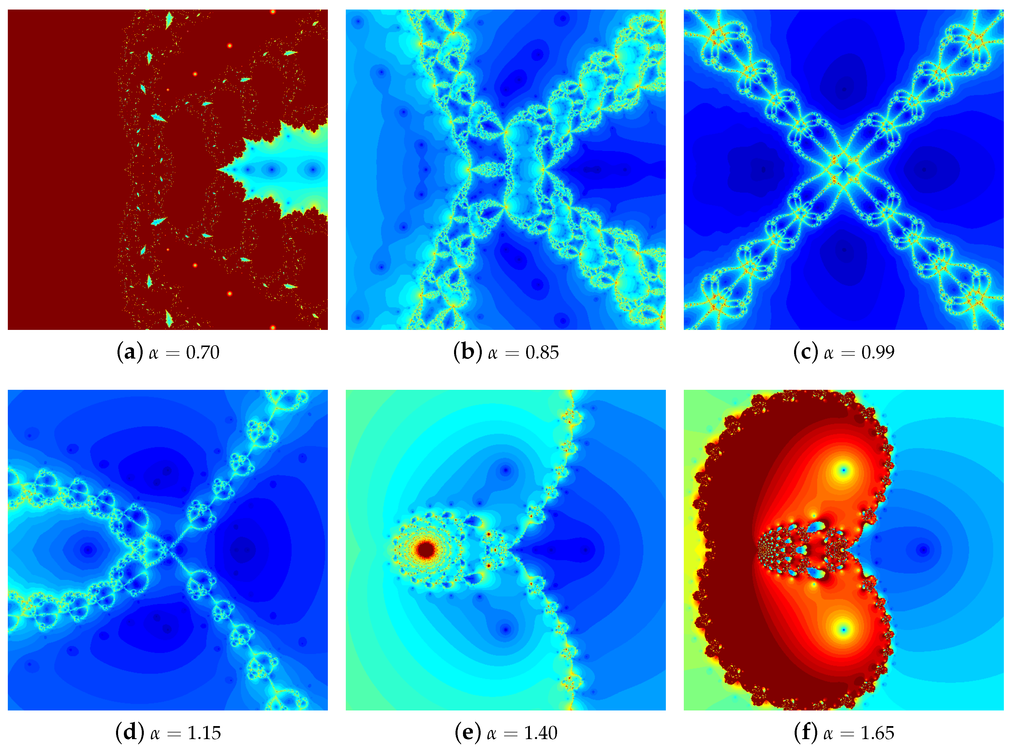
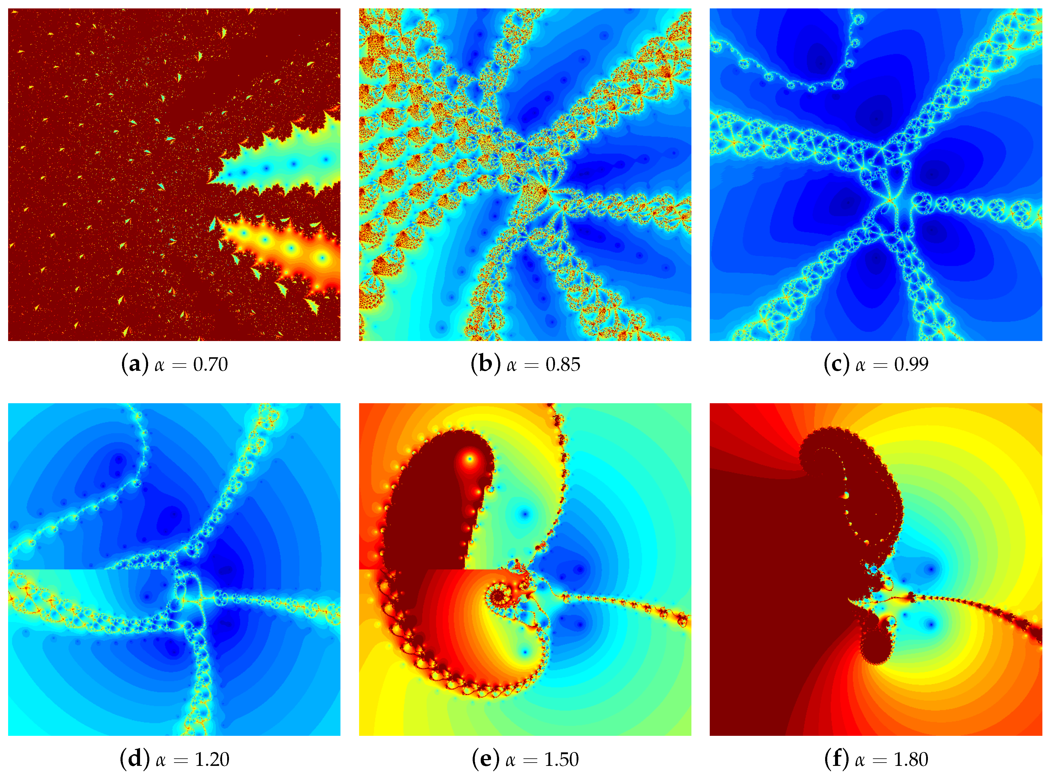
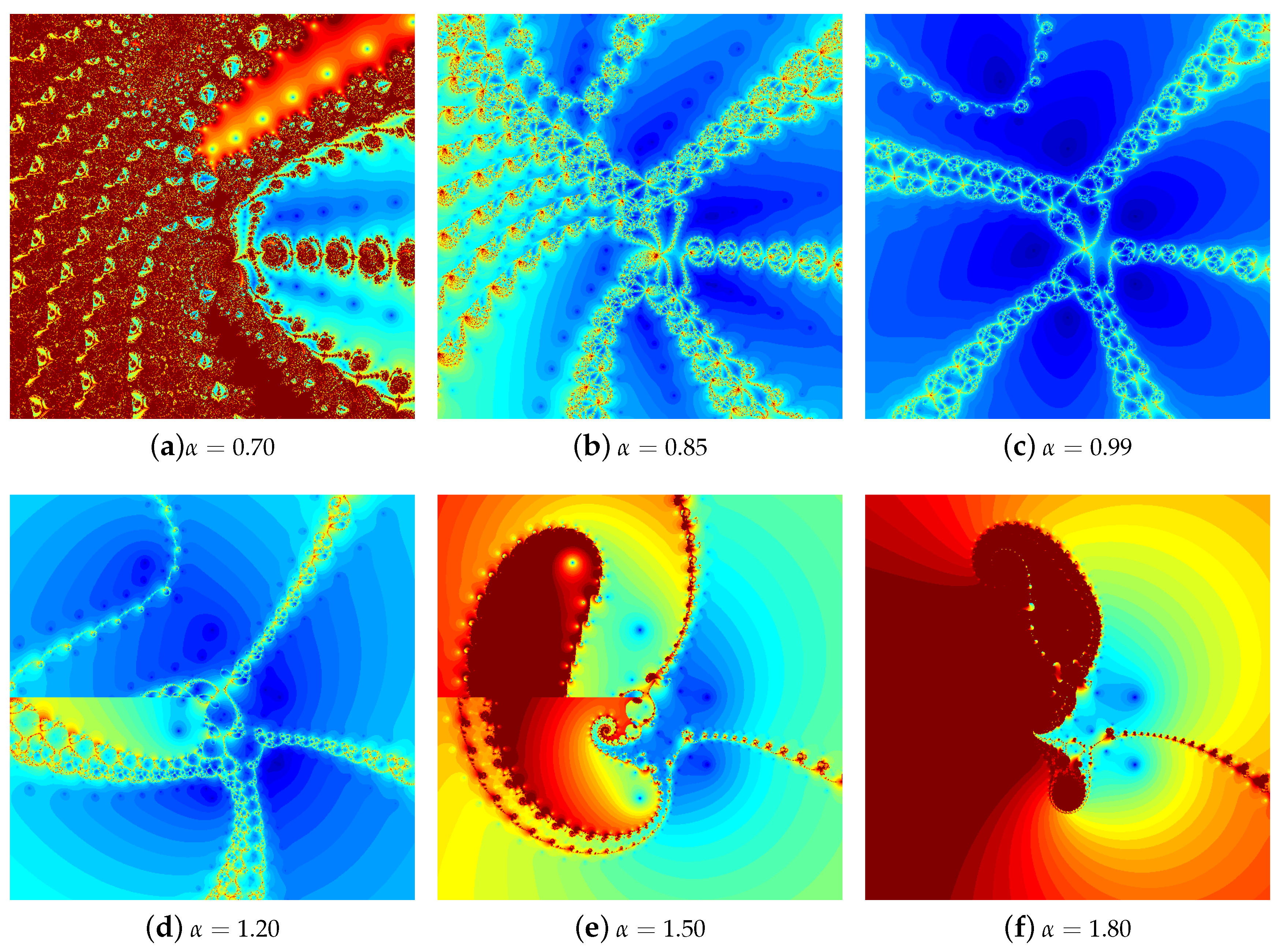
The polynomiographs obtained with the iteration colouring for the same values of $\alpha$ as for the basins of attraction are presented in Figure 24 and Figure 25. From these polynomiographs we can observe that the braids behave in a similar fashion as in the case of basins of attraction. For $\alpha <1$, the left braids are moving away from the real axis and they are splitting, whereas, for $\alpha >1$, the braids are getting smaller and, moreover, they are bending and joining together, forming interesting patterns, especially in Figure 24e and Figure 25e. Furthermore, with the change of the $\alpha$-order the dynamics of the methods also changes. The change is different for miscellaneous values of this parameter. For the value near 1 (Figure 24c and Figure 25c), we can observe only a small change in dynamics in comparison to the classical Newton’s method (Figure 21b). When we decrease the value to $0.85$, we see increase in dynamics in all areas of the polynomiographs (see Figure 24b and Figure 25b). Then, for $\alpha =0.70$, we see a low dynamic for both methods (Figure 24a and Figure 25a) because most of the points in the considered area do not converge, i.e., the points with red colour. In this case, the RL-Newton method has much lower dynamics than the C-Newton one. Increasing the value of $\alpha$ above 1 changes the dynamics in the areas outside the braids. For both methods, the dynamics is increasing in the areas laying on the right side. In the left part of the polynomiographs, the dynamics is decreasing due to the presence of points that do not converge to any root.

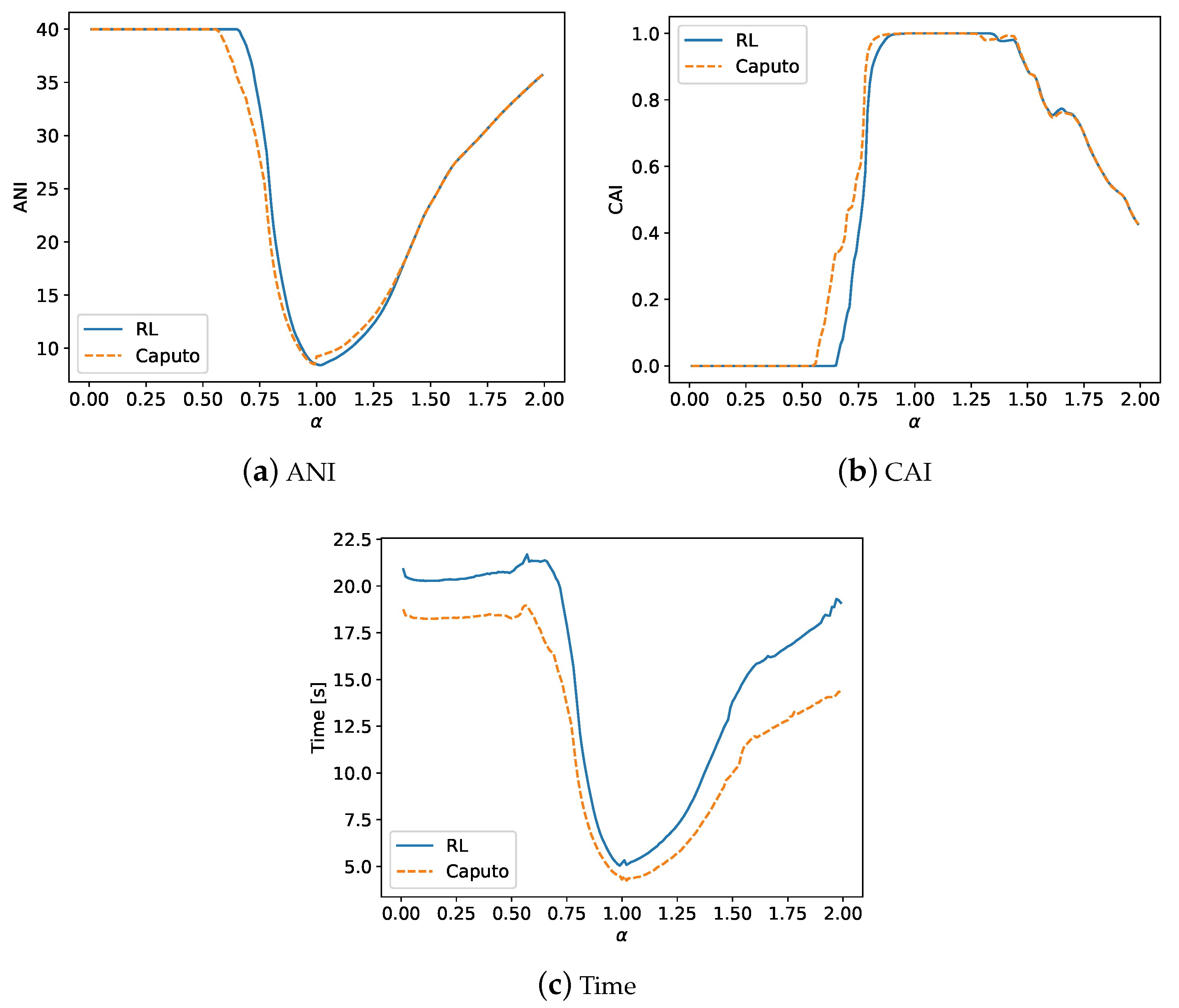
The numerical results obtained for $p_6$ are presented in Figure 26. In Figure 26a, we see the results for ANI. The lowest value of ANI is obtained for values of $\alpha$ near 1. The minimal value of ANI, equal to $8.406$ for the RL-Newton method, is attained at $\alpha =1.02$, whereas the minimal value $8.480$ for the C-Newton method is attained at $\alpha =0.99$. By comparing these results to the classical Newton’s method ($7.984$), we see that the ANI value for the methods with fractional derivatives is larger. When we look at the plots, we see that both methods have almost identical behaviour. For $\alpha <1$, the C-Newton method obtained slightly lower values of ANI, whereas, for $\alpha >1$, the situation is inverted, i.e., the RL-Newton method obtained lower value, but only for $\alpha \in (1.0,1.39)$. Both methods lose their convergence properties, i.e., obtain the maximal number of iterations for all points in polynomiographs equal to 40, for different values. The threshold for the RL-Newton method is equal to $0.57$ and for the C-Newton method is equal to $0.53$. The results obtained for CAI are presented in Figure 26b. Similar to the previous polynomials, both methods obtained the highest values of CAI equal to $1.0$ in the neighbourhood of $\alpha =1.0$, i.e., for $\alpha \in (0.96,0.99)\cup (1.01,1.33)$ and $\alpha \in (0.94,1.22)$ for the RL-Newton and C-Newton methods, respectively. For $\alpha >1.0$, both methods behave almost identically, whereas, for $\alpha <1$, we see that the C-Newton method obtains greater values of CAI. The decrease of the value of CAI outside the intervals in which the methods obtained the values equal to $1.0$ is very rapid. Moreover, for $\alpha <0.65$ in the case of the RL-Newton method and $\alpha <0.55$ in the case of the C-Newton method, the value of CAI is equal to $0.0$, thus, for these values of $\alpha$, the methods do not converge to any root. In Figure 26c, we see the plots with the times of generation of the polynomiographs. The best times for both methods, as in the previous examples, are near $\alpha =1.0$, i.e., at $\alpha =1.02$ they are equal to $5.081$ s and $4.244$ s for the RL-Newton and C-Newton method, respectively. These times are higher than for the classical Newton’s method ($1.368$ s). By increasing or decreasing the value of $\alpha$ above or below $1.02$, we can observe a rapid increase of the generation time. Both methods behave very similarly, but the growth in the case of the C-Newton method is smaller than for the RL-Newton method. Both methods obtained the longest times for $\alpha <1.02$, i.e., the RL-Newton obtained time equal to $21.684$ s at $\alpha =0.57$, whereas the C-Newton method obtained the time equal to $18.961$ s at $\alpha =0.56$. Irrespective of the $\alpha$ value, the C-Newton method obtains shorter times than the RL-Newton method.

4.2. Summary of the Experiments

The polynomiographs (the basins of attraction and the polynomiographs with the iteration colouring) generated with the fractional methods for $\alpha$ approaching to 1 from the above or from the below are approaching the set of polynomiographs obtained for the classical Newton’s method. When we move away from $\alpha =1.0$ in either direction, we can observe that the shapes of the polynomiographs change in a significant way in the left part of the images. Together with the shape change, the dynamics of the methods also changes. The dynamics is high for $\alpha \in (0.8,1.4)$, and then the dynamics is lower due to the presence of many points for which the methods do not converge to any root. For the basins of attraction, when we move away from $\alpha =1.0$, some of the roots are not found by the methods, i.e., the basins of attraction of these roots just vanish. The polynomiographs for $p_2,p_3,p_4$ are not symmetric as in the classical Newton method and contain more areas with turbulences and chaos. They look more “fractally”. Moreover, in many of the polynomiographs, we can observe a straight line along negative real axis, e.g., in Figure 10d, Figure 11d, Figure 16e and Figure 17e, among others. These straight lines might be related with the choice of the negative real half-axis as the branch cut line. From the numerical experiments, we can observe that the C-Newton method behaves better than the RL-Newton method. The former method obtains shorter times, needs fewer iterations on average (lower values of ANI), and, at the same time, more points are converging (greater value of CAI) to the roots. The best values of each of the three measures are attained for $\alpha$ in the neighbourhood of $1.0$.

5. Conclusions and Future Work

In this paper, some modifications of the root-finding process based on fractional Riemann–Liouville and Caputo derivatives are investigated via polynomiographs. For several polynomials, the basins of attractions and the images coloured with respect to the number of iterations together with the plots showing the dependence of the $\alpha$-order on the three different measures (ANI, CAI and the generation time) are presented.

In general, fractional derivatives in the complex plane can be well-defined not only by choosing the principal branch of multivalued expressions that are in their definitions, as usually is implemented in programming languages and CAS systems. Therefore, the question concerning the behaviour of the considered methods with fractional derivatives for the choice of the other branches different from the principal one is an interesting.

As in [5], the results of this paper can be further modified by the use of multi-parameter iterations, various convergence tests or different colour maps. In addition, the application of the higher order methods based on the Basic or Euler–Schröder families of iterations [2] with non-standard iteration processes lead to further possible modifications. Next, it is worth checking experimentally the use of complex parameters instead of real ones in multi-parameter iterations. Such a change probably does not destabilise convergence of the investigated processes. At the end, the artistic aspects of polynomiographs should be mentioned. They are images looking nicely and their appearance is greatly influenced by the different colour palettes used to generate them.

References

- Mandelbrot, B. The Fractal Geometry of Nature; W.H. Freeman and Company: New York, NY, USA, 1983. [Google Scholar]
- Kalantari, B. Polynomial Root-Finding and Polynomiography; World Scientific: Singapore, 2009. [Google Scholar] [CrossRef]
- Kalantari, B. Polynomiography: From the Fundamental Theorem of Algebra to Art. Leonardo 2005, 38, 233–238. [Google Scholar] [CrossRef]
- Gdawiec, K.; Kotarski, W. Polynomiography for the Polynomial Infinity Norm via Kalantari’s Formula and Nonstandard Iterations. Appl. Math. Comput. 2017, 307, 17–30. [Google Scholar] [CrossRef]
- Gdawiec, K.; Kotarski, W.; Lisowska, A. Polynomiography Based on the Non-standard Newton-like Root Finding Methods. Abstr. Appl. Anal. 2015, 2015, 797594. [Google Scholar] [CrossRef]
- Ardelean, G.; Cosma, O.; Balog, L. A Comparison of Some Fixed Point Iteration Procedures by using the Basins of Attraction. Carpath. J. Math. 2016, 32, 277–284. [Google Scholar]
- Chun, C.; Neta, B. Comparison of Several Families of Optimal Eighth Order Methods. Appl. Math. Comput. 2016, 274, 762–773. [Google Scholar] [CrossRef]
- Chun, C.; Neta, B. On the New Family of Optimal Eighth Order Methods Developed by Lotfi et al. Numer. Algorithms 2016, 72, 636–637. [Google Scholar] [CrossRef]
- Ardelean, G.; Balog, L. A Qualitative Study of Agarwal et al. Iteration Procedure for Fixed Points Approximation. Creat. Math. Inform. 2016, 25, 135–139. [Google Scholar]
- Gdawiec, K. Fractal Patterns from the Dynamics of Combined Polynomial Root Finding Methods. Nonlinear Dyn. 2017, 90, 2457–2479. [Google Scholar] [CrossRef]
- Brambila-Paz, F.; Torres-Hernandez, A. Fractional Newton–Raphson Method. 2017. Available online: https://arxiv.org/abs/1710.07634 (accessed on 28 July 2019).
- Brambila-Paz, F.; Torres-Hernandez, A.; Iturrarán-Viveros, U.; Caballero-Cruz, R. Fractional Newton-Raphson Method Accelerated with Aitken’s Method. 2018. Available online: https://arxiv.org/abs/1804.08445 (accessed on 28 July 2019).
- Abel, N. Opløsning af et Par Opgaver ved Hjælp af bestemte Integraler. Mag. Naturvidensk. 1823, 2, 205–215. [Google Scholar]
- Sun, H.; Zhang, Y.; Baleanu, D.; Chen, W.; Chen, Y. A New Collection of Real World Applications of Fractional Calculus in Science and Engineering. Commun. Nonlinear Sci. Numer. Simul. 2018, 64, 213–231. [Google Scholar] [CrossRef]
- Herrmann, R. Fractional Calculus: An Introduction for Physicists, 2nd ed.; World Scientific: Singapore, 2014. [Google Scholar] [CrossRef]
- Hilfer, R. Applications of Fractional Calculus in Physics; World Scientific: Singapore, 2000. [Google Scholar] [CrossRef]
- Oldham, K.; Spanier, J. The Fractional Calculus: Theory and Applications of Differentiation and Integration to Arbitrary Order. In Mathematics in Science and Engineering; Academic Press: San Diego, CA, USA, 1974; Volume 111. [Google Scholar]
- Samko, S.; Kilbas, A.; Marichev, O. Fractional Integrals and Derivatives: Theory and Applications; Gordon and Breach Science Publishers: Amsterdam, The Netherlands, 1993. [Google Scholar]
- Wheeler, N. Construction and Physical Application of the Fractional Calculus. 1997. Available online: https://www.reed.edu/physics/faculty/wheeler/documents/Miscellaneous%20Math/Fractional%20Calculus/A.%20Fractional%20Calculus.pdf (accessed on 28 July 2019).
- Ishteva, M. Properties and Applications of the Fractional Caputo Operator. Master’s Thesis, Department of Mathematics, Universität Karlsruhe, Karlsruhe, Germany, 2005. [Google Scholar]
- Diethelm, K. The Analysis of Fractional Differential Equations; Springer: Heidelberg, Germany, 2010. [Google Scholar]
- Vance, D. Fractional Derivatives and Fractional Mechanics. 2014. Available online: https://sites.math.washington.edu/~morrow/336_14/papers/danny.pdf (accessed on 28 July 2019).
- Chong, Y. Branch Points and Branch Cuts. 2016. Available online: http://www1.spms.ntu.edu.sg/~ydchong/teaching/07_branch_cuts.pdf (accessed on 28 July 2019).
- Le Bourdais, F. Understanding Branch Cuts in the Complex Plane. 2016. Available online: http://flothesof.github.io/branch-cuts-with-square-roots.html (accessed on 28 July 2019).
- Kahan, W. Branch Cuts for Complex Elementary Functions or Much Ado About Nothing’s Sign Bit. In Proceedings of the Joint IMA/SIAM Conference on the State of the Art in Numerical Analysis; Iserles, A., Powell, M., Eds.; Clarendon Press: New York, NY, USA, 1987; pp. 165–211. [Google Scholar]
- England, M.; Cheb-Terrab, E.; Bradford, R.; Davenport, J.; Wilson, D. Branch Cuts in Maple 17. ACM Commun. Comput. Algebra 2014, 48, 24–27. [Google Scholar] [CrossRef]
- Munkhammar, J. Fractional Calculus and the Taylor-Riemann Series. Rose Hulman Undergrad. Math. J. 2005, 6, 6. [Google Scholar]
- Ortigueira, M.; Rodríguez-Germá, L.; Trujillo, J. Complex Grünwald-Letnikov, Liouville, Riemann-Liouville, and Caputo Derivatives for Analytic Functions. Commun. Nonlinear Sci. Numer. Simul. 2011, 16, 4174–4182. [Google Scholar] [CrossRef]
- Li, C.; Daoa, X.; Guoa, P. Fractional Derivatives in Complex Planes. Nonlinear Anal. 2009, 71, 1857–1869. [Google Scholar] [CrossRef]
- Ortigueira, M.D. A Coherent Approach to Non-integer Order Derivatives. Signal Process. 2006, 86, 2505–2515. [Google Scholar] [CrossRef]
Figure 1.
The plots of the (a) real and (b) imaginary parts of -order RL derivative of .
Figure 2.
The colour map used in the experiments.
Figure 3.
The polynomiographs of the classical Newton’s method for .
Figure 4.
The basins of attraction for the RL-Newton method for and various values of .
Figure 5.
The basins of attraction for the C-Newton method for and various values of .
Figure 6.
The iteration colouring for the RL-Newton method for and various values of .
Figure 7.
The iteration colouring for the C-Newton method for and various values of .
Figure 8.
The numerical results for and the different measures.
Figure 9.
Figure 10.
Figure 11.
Figure 12.
Figure 13.
Figure 14.
Figure 15.
Figure 16.
Figure 17.
Figure 18.
Figure 19.
Figure 20.
Figure 21.
Figure 22.
Figure 23.
Figure 24.
Figure 25.
Figure 26.
© 2019 by the authors. Licensee MDPI, Basel, Switzerland. This article is an open access article distributed under the terms and conditions of the Creative Commons Attribution (CC BY) license (http://creativecommons.org/licenses/by/4.0/).
Share and Cite
MDPI and ACS Style
Gdawiec, K.; Kotarski, W.; Lisowska, A. Visual Analysis of the Newton’s Method with Fractional Order Derivatives. Symmetry 2019, 11, 1143. https://doi.org/10.3390/sym11091143
AMA Style
Gdawiec K, Kotarski W, Lisowska A. Visual Analysis of the Newton’s Method with Fractional Order Derivatives. Symmetry. 2019; 11(9):1143. https://doi.org/10.3390/sym11091143
Chicago/Turabian StyleGdawiec, Krzysztof, Wiesław Kotarski, and Agnieszka Lisowska. 2019. "Visual Analysis of the Newton’s Method with Fractional Order Derivatives" Symmetry 11, no. 9: 1143. https://doi.org/10.3390/sym11091143
Note that from the first issue of 2016, this journal uses article numbers instead of page numbers. See further details here.