A Novel Two-Stage Heuristic for Solving Storage Space Allocation Problems in Rail–Water Intermodal Container Terminals

Abstract

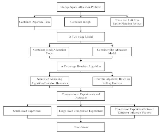
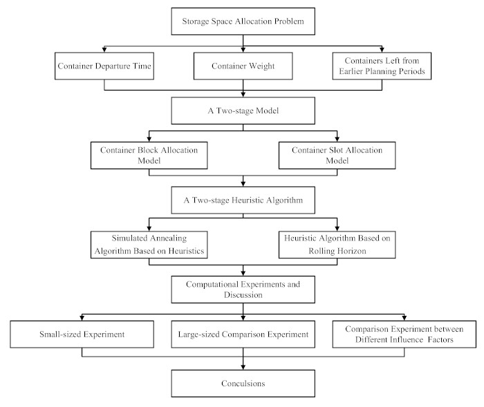
In the past, most researchers have paid attention to the storage space allocation problem in maritime container terminals, while few have studied this problem in rail–water intermodal container terminals. Therefore, this paper proposes a storage space allocation problem to look for a symmetry point between the efficiency and effectivity of rail–water intermodal container terminals and the unbalanced allocations and reallocation operations of inbound containers in the railway operation area, which are two interactive aspects. In this paper, a two-stage model on the storage space allocation problem is formulated, whose objective is to balance inbound container distribution and minimize overlapping amounts, considering both stacking principles, such as container departure time, weight and stacking height, and containers left in railway container yards from earlier planning periods. In Stage 1, a novel simulated annealing algorithm based on heuristics is introduced and a new heuristic algorithm based on a rolling horizon approach is developed in Stage 2. Computational experiments are implemented to verify that the model and algorithm we introduce can enhance the storage effect feasibly and effectively. Additionally, two comparison experiments are carried out: the results show that the approach in the paper performs better than the regular allocation approach and weight constraint is the most important influence on container storage.

1. Introduction

With the trend of world economy and trade globalization, container transportation, regarded as one of the most significant modern freight means of transportation, has become widespread all around the world. Intermodal transportation, as one of the most important container transportation modes, has become an increasing concern, especially rail–water intermodal transportation.

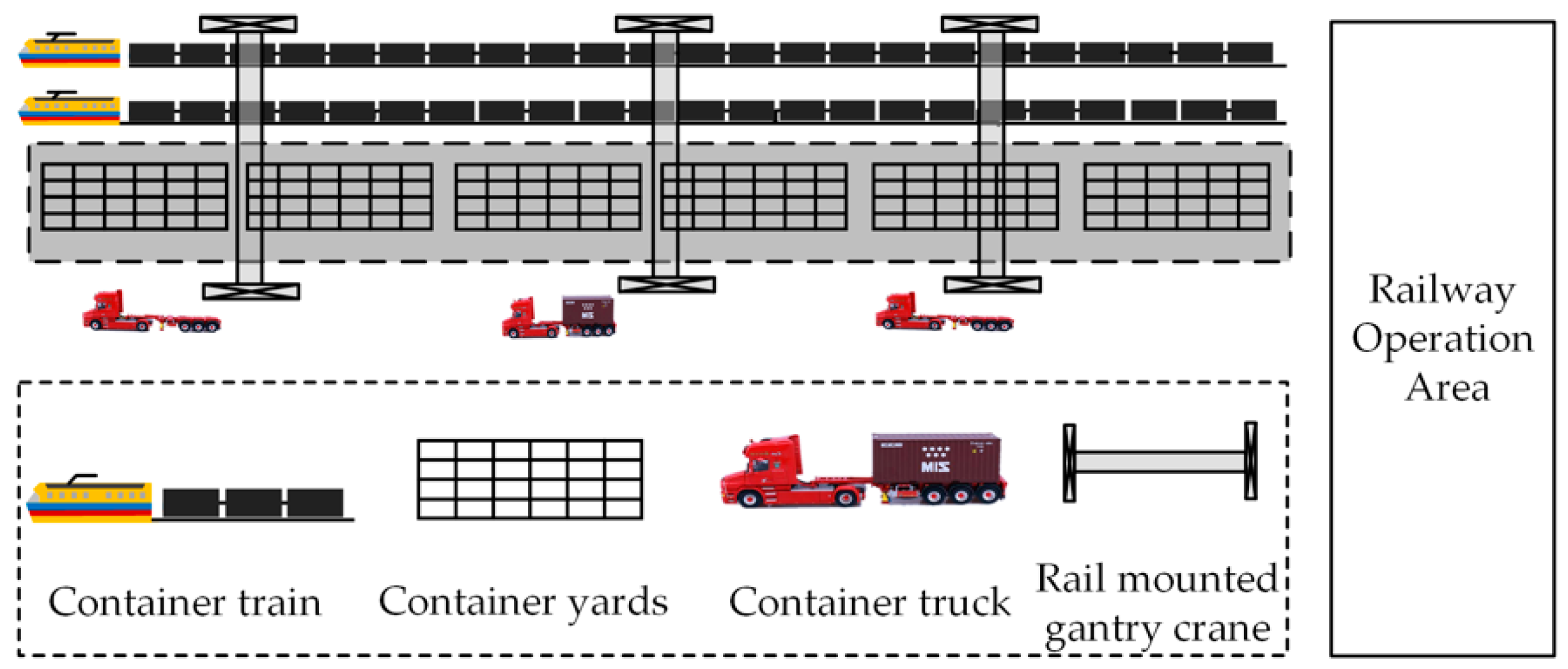
Rail–water intermodal container terminals (RWICTs), as an interface between the seaside area and landside area, are composed of five parts. These five parts are the quayside area, container yards, travelling paths, gates and railway operation area. The railway operation area is the place to store and handle containers transported by rail. Meanwhile this area has its own container yards, called railway container yards, which are usually adjacent to railway tracks. Thus, rail mounted gantry cranes (RMGCs) not only handle containers, but also stack containers.

Additionally, rational utilization and allocation of handling equipment and storage space in the railway operation area are two main dispatcher’s issues. Meanwhile, because the arrival and departure time of a train can hardly coordinate with the arrival and departure time of ships, both outbound and inbound containers generally need storing in railway container yards. Consequently, our paper concentrated on the storage space allocation problem (SSAP), which is an essential basis and constraint for other resources utilization in the railway operation area.

SSAP usually can be decomposed into two sub-problems: one is the container block allocation problem (CBAP) and the other is the container slot allocation problem (CSAP). The former aims at balancing the number of containers in different blocks by selecting the optimal block for containers from container yards. The objective of the latter is to reduce reallocation operations of containers by assigning containers into the optimal slot in the assigned bays of container blocks. Generally, dispatchers should assign containers into various blocks first and then allocate them into slots of the blocks, so CBAP should be solved before CSAP. Therefore, we formulated the model of CBAP first to determine optimal blocks for containers and then developed the CSAP model to obtain specific positions for containers.

Hence, the contribution of this paper is described as follows. Firstly, the whole storage space allocation problem for inbound containers was studied together, which considered both the container block allocation problem and container slot allocation problem. Secondly, not only storage principles were considered in the paper, but containers left from earlier planning horizons were taken into account. Thirdly, a novel two-stage solution was introduced to solve SSAP. Finally, some experiments were proposed to verify that the model and algorithm in the paper were feasible and effective in improving the storage effect, and meanwhile verified that the proposed approach was better than the regular allocation approach and weight constraint should be considered firstly in storing containers.

The rest of this paper is organized as follows: the related literature is presented in Section 2. Section 3 describes SSAP and a two-stage model is formulated in the fourth section. Section 5 develops a simulated annealing algorithm based on heuristics (SAAH) and a heuristic algorithm based on a rolling horizon (HARH), based on Reference [1], is used to solve the proposed model. Computational experiments are analyzed in the sixth section and eventually Section 7 concludes the paper.

2. Literature Review

According to [2], there are four main decision problems that are paid attention to for storage yard operations:

• yard design, including material handling equipment selection and storage yard layout (e.g., [3,4]);
• storage space assignment to containers (e.g., [5,6]);
• material handling equipment dispatching and routing to serve the storage and/or retrieval requests (e.g., [7,8]);
• optimizing the reshuffling of containers (e.g., [9,10]).

In our paper, we mainly concentrated on storage space assignment to containers.

Most of the literatures study SSAP in marine container terminals. A dynamic programming model has been introduced to assign arriving export containers to storage yards, considering its weight [11]. Kim et al. [12] discusses SSAP of outbound containers (OCs) in maritime container terminals and introduces two heuristic algorithms to solve the proposed problem. Yan et al. also studies SSAP in maritime container terminals. Based on an advanced handling strategy, the allocation process of inbound containers (ICs) is investigated and analyzed, and a multi-objective integer programming model is developed, considering the real-time strategic planning and intense loading and unloading synchronously [13]. A yard storage allocation problem has been developed in a transshipment hub with the aim of reducing re-handling and a consignment strategy and two heuristic algorithms are proposed to solve the problem [14]. Mckendall [15] presents construction algorithms and a tabu search heuristic algorithm to optimize the space/resource assignments during the implementation of project activities. Then they study the dynamic space allocation problem on allocating containers to locations of the storage yard to minimize the reallocation cost and introduce a three tabu search heuristic algorithm [16].

A genetic algorithm has been introduced to solve an extended SSAP efficiently in a maritime container terminal, considering the types of containers affecting container allocation in blocks [17]. Choe et al. [18] propose an approach to efficiently search an intra-block remarshaling plan so that the interference between stacking cranes is minimized, which is free from reallocation during both loading and remarshaling operation. Yu et al. [19] study CBAP considering several optimization models under storing strategies and used simulation to verify their models and solution approaches. A novel method has been introduced to balance the workload among different blocks and reduce traveling distance of inner trucks between blocks and berths. They develop an ant-based control algorithm to solve the problem [20]. A systematic approach called “space allocation given long-term plan” has been proposed to balance current and future effects of short-term planning and two storage strategies are introduced to evaluate their approach [21].

All the literatures above study SSAP in maritime container terminals and focus more on CBAPs, while they neglect CSAPs, which also affect the efficiency of RWICTs. Meanwhile, they only consider allocation operation constraints and workload constraints; however, besides these constraints, other constraints, such as specific allocation position constraints and allocation preference constraints, were also taken into consideration in our paper. In addition, most solution algorithms are heuristic algorithms, while in our paper we introduced a novel SAAH to solve CBAP.

What is more, only a few pieces of literature concentrate on CSAPs or RWICTs. Zheng et al. [22] focus on CSAPs under the inbound and outbound container mixed storage mode, considering containers’ processing priority based on rolling plans to decrease the container relocation rate and enhance loading efficiency. They adopt a heuristic algorithm to solve their problem. However, they only consider weight priority when stacking containers. Wang et al. [23] study SSAP under the inbound and outbound container mixed storage mode in railway container terminals and develop a two-stage optimization model and a heuristic algorithm to solve this problem. Then in 2014 they consider SSAP of ICs in a railway container terminal and formulate a novel model and algorithm for this problem. However, they only consider departure time and the algorithm used in their paper has a heuristic approach [24].

Liu et al. [25] develop a multi-objective optimization model of CSAP to balance the number of each stack and lessen the re-handling and storage cost, considering uncertain arrival time of OCs. Heuristic optimization algorithms are introduced to solve the proposed problem. However, they neglect the departure time of containers and stacking height constraint. Ji et al. [26] concentrate on the container allocation problem during loading and unloading processes on railway center terminals and establish a dynamic container allocation optimization model. However, they ignore some other stacking principles except departure time. Li et al. [27] study CSAP considering the storage plan in RWICTs but they do not consider height difference between two adjacent stacks and assume that bays are all empty before stacking containers. However, it is irrational to assume all the bays in RWICTs are empty; there must be some containers left from early planning periods.

According to all the literatures above, specific literatures on rail–water intermodal container terminals are scarce. Some researchers do consider some principles to store containers in SSAP; however, they only focus on one of them, seldom considering all of them. Moreover, most researchers neglect containers left from earlier planning periods in container yards, which can also affect the stacking state.

Consequently, in this paper, we studied SSAP of ICs in RWICTs, including not only CBAP to balance the allocation of inbound containers, but also CSAP to reduce the reshuffling operations. Meanwhile, not only the stacking principles, for example container weight, departure time and stacking height difference between two neighboring stacks, were considered in our paper, but containers left from earlier planning periods were also considered.

3. Problem Description

3.1. Related Descriptions

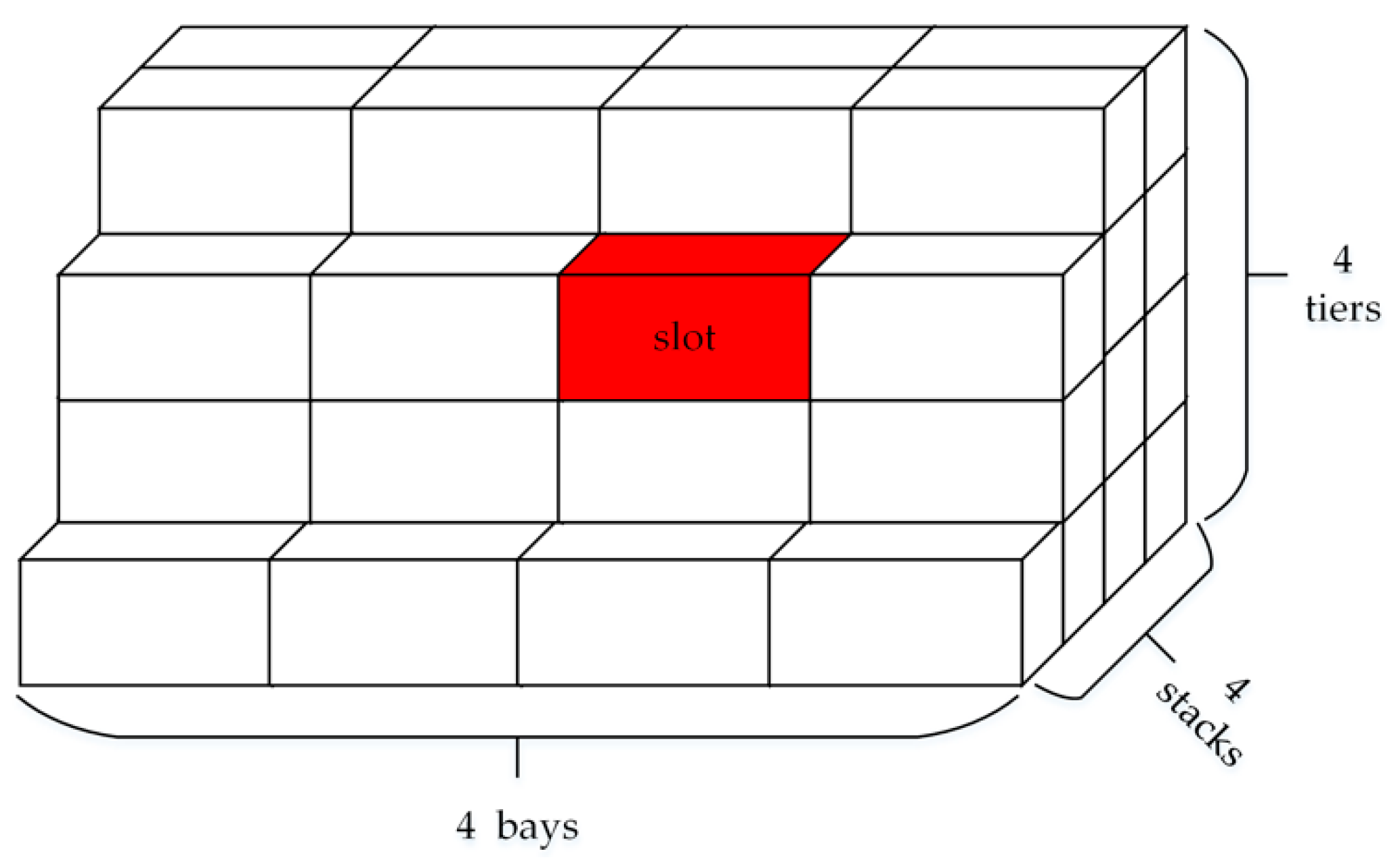
Before formulating a mathematical model, some descriptions used in the mathematical model are to be introduced firstly. As you can see, railway container yards in a RWICT are adjacent to railway tracks in Figure 1 and Figure 2, which consist of some blocks. Each block is made up of several parallel bays. Each bay has several stacks and each stack has several tiers.

There are two storage modes in RWICTs: one is the inbound and outbound containers mixed storage mode and the other one is the inbound and outbound containers separated storage mode. The former mode can save space for container yards; however, it may raise the workload of handling equipment and cause the efficiency of RWICTs to be too low. What is more, this mode also requires high quality stacking rules, which increases the difficulty for dispatchers. Meanwhile, in most Chinese container terminals, ICs and OCs are stored separately for ease of handling and stacking operations, such as Chongqing RWICT and Dalian RWICT, which were the RWICTs we investigated. Therefore, we adopted the second storage mode in the paper, and we set ICs as our research object.

In our paper, there were two statuses of ICs in different handling operations:

• ICs on vessels or inner trucks waiting for discharging and assigning to the railway container yard, called VDs;
• ICs have been already stored in the railway container yard, waiting for loading onto trains, called TPs;

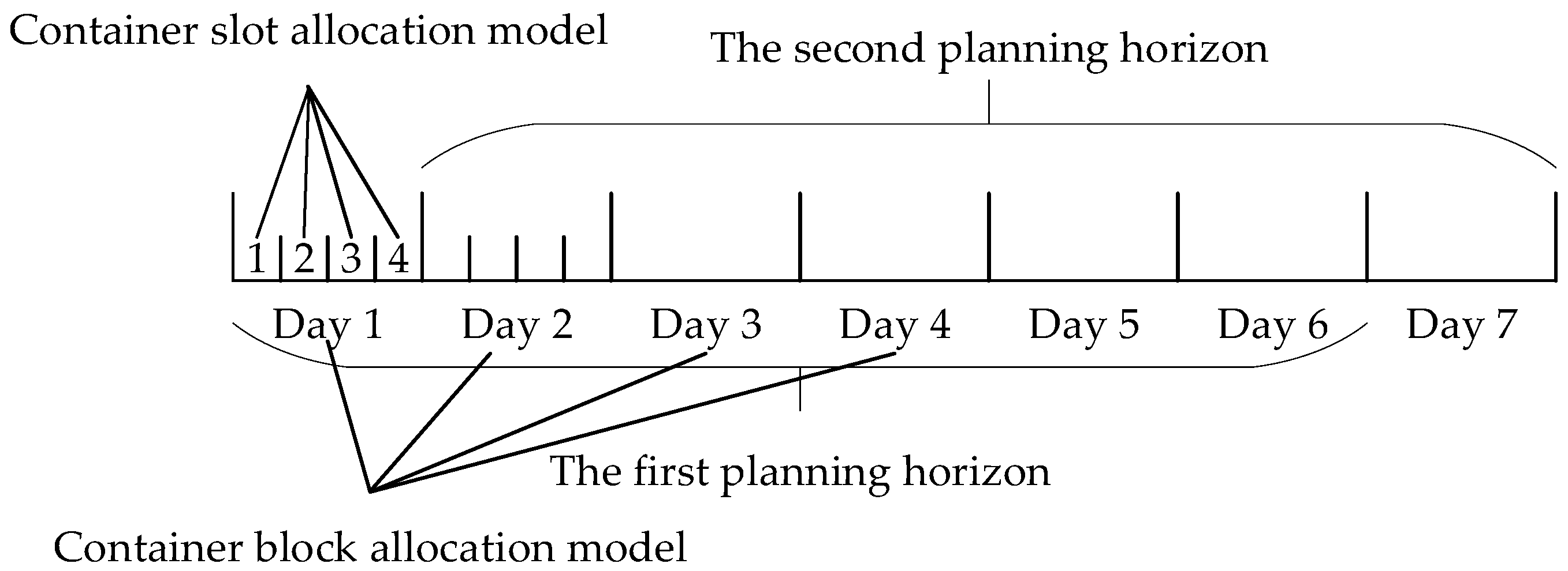
Since RWICTs operate continuously for a whole year, it is essential to select a fixed period as a planning horizon so that the number of containers can be counted easily. Therefore, according to Reference [5], a fixed horizon in the immediate future was introduced at each planning epoch and the plan was executed accordingly up to the next planning epoch; then a new plan was formulated based on the latest information and this mode continued. An example of the rolling planning horizon is shown in Figure 3. CBAP is performed in each planning epoch of the planning horizon, while CSAP is performed in each period of the planning epoch.

3.2. Overlapping Amount

Since CSAP is to choose specific positions for containers, some storage principles should be considered, which may influence the stacking state and increase reallocation operations:

• Since heavier containers are stored below lighter containers in the containership, the lighter containers are loaded before the heavier containers. Therefore, in the railway container yards the lighter containers should be stored below the heavier containers to ensure the safety and stability of the storage.
• In order to ensure containers with an early departure time can be put onto trains early, containers with an earlier departure time need to be stacked on containers with later departure times.
• Height difference between two neighboring stacks in the same bay should not exceed three.

If containers do not meet the first or the second storage principle, then the overlapping amount increases, which stands for the number of reallocation operations during the stacking process to some degree. To simplify the description of container information, the actual weight and departure time of containers were converted into weight and departure time priority, separately. The lighter the container was, the smaller the weight priority was; the earlier the container departure time was, the smaller the departure time priority was.

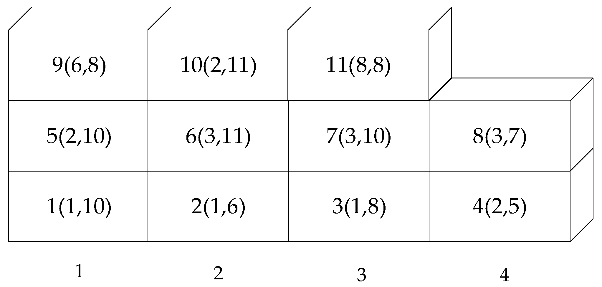
To calculate the overlapping amount, a couple of containers were introduced, which referred to two containers in upper and lower relationships in the same stack. Therefore, the calculation rule of overlapping amount was that if a couple of containers violated one of the first two storage principles, the total overlapping amount increased.

Figure 4 shows an example of the overlapping amount calculation. The number out of the brackets in Figure 4 stands for the number of a container while the numbers in brackets in Figure 4 mean the weight priority and departure time priority. According to the first storage principle and the calculation rule of the overlapping amount, the overlapping amount is 0, 2, 1 and 1 in Stack 1, 2, 3 and 4, respectively. For example, in Stack 2, the weight priority of Container 10 exceeds the weight priority of Container 6, and Container 6 departs later than Container 2; although Container 10 departs later than Container 2, they do not satisfy the definition of a couple of containers. Thus, the overlapping amount in Stack 2 is 2.

What is more, to ensure that there were some slots available to re-handle containers, it was regulated that not all the stacks in the railway container yard could reach the maximum height and there must be enough empty slots, which were usually set aside in the nearest side of each bay, to allocate the re-handled containers. Thus, the relationship between tiers and empty slots is shown in

Table 1. The relationship between tiers and empty slots.

Tiers	Empty Slots
3	2
4	3
5	4
$t$	$t-1$

. As shown in Table 1, if one stack had four-tier containers, and the container in the bottom needed picking up, then the containers on it should have been reallocated to some empty slots. Therefore, there must have been three empty slots left.

4. Problem Formulation

According to problem description above, we studied SSAP and formulated a two-stage model for SSAP, considering some storage principles and containers left from early periods. The first stage was container block allocation, which aimed at balancing the workload among different blocks and evenly assigned ICs into the block. Stage 2 was container slot allocation, the objective of which was to reduce overlapping amounts of ICs.

4.1. Assumptions

There were four assumptions for the formulation of the problem in the paper:

• All the containers were assumed to have the same size and meanwhile special containers, such as refrigerated containers and hazardous containers, were not considered in our paper;
• The positions and information of the containers left from earlier planning horizons were known before;
• The information of the new arrival containers, such as weight and departure time, were known before;
• There was enough handling equipment to handle and store containers in the railway operation area.

4.2. Container Block Allocation Model

4.2.1. Notations and Variables

Notations and variables used in the container block allocation model are shown as follows.

$IB$: the total number of IC blocks;

$M$: the total number of planning periods in a planning epoch;

$C_n$: the theoretical storage capacity of the block $n$, $1\le n\le IB$;

$w_n$: the storage coefficient of the block $n$, $1\le n\le IB$;

$V_{nm}$: the number of ICs in the block $n$ at the beginning of the period $m$, $1\le n\le IB,1\le m\le M$;

$V{D}_{nm}$: the number of VDs allocated to the block $n$ during the period $m$, $1\le n\le IB,1\le m\le M$;

$V{D}_{nmk}$: the number of VDs assigned to the block $n$ during the period $m$ and to be loaded onto trains during the period $m+k$, $1\le n\le IB,1\le m\le M,0\le k\le M-m$;

$V{D}_{nm}{}^{\prime }$: the number of VDs assigned to the block $n$ during the period $m$ and to be loaded onto trains after this planning epoch, $1\le n\le IB,1\le m\le M$;

$T{P}_{nm}$: the number of TPs in the block $n$ that are loaded onto trains during the period $m$, $1\le n\le IB,1\le m\le M$;

$T{P}_{nm}^0$: the number of TPs in the block $n$ at the beginning of the period $m$, $1\le n\le IB,1\le m\le M$;

$OF{V}_1$: the objective value of CBAP.

4.2.2. Objective

Based on the description of the problem above, the objective function is shown below.

$$OF{V}_1=Min {\displaystyle \sum _{m=1}^M{\displaystyle \sum _{n=1}^{IB}\left|(V{D}_{nm}+T{P}_{nm})-\frac{{\displaystyle \sum _{n=1}^{IB}(V{D}_{nm}+T{P}_{nm})}}{IB}\right|}}.$$

(1)

Equation (1) shows the objective function of the paper, which indicates that the mean difference of the workload in all the blocks is minimized to balance each block’s workload.

4.2.3. Constraints

To guarantee the feasibility and operability of all solutions, the constraints in the problem are as follows.

1. Constraints on VDs

$$V{D}_{nm}={\displaystyle \sum _{k=0}^{M-m}V{D}_{nmk}+V{D}_{nm}{}^{\prime }},n=1,2,\dots ,IB,m=1,2,\dots ,M.$$

(2)

Constraint (2) implies that the total number of VDs allocated to the block $n$ during the period $m$ is the sum of containers allocated to the block $n$ during the period $m$ and to be loaded onto trains during the period $m+k$ and after this planning epoch.

2. Constraints on TPs

$$T{P}_{nm}=T{P}_{nm}^0+{\displaystyle \sum _{k=0}^{m-1}V{D}_{n(m-k)k}},n=1,2,\dots ,IB,m=1,2,\dots ,M.$$

(3)

Constraint (3) indicates that the total number of TPs in the block $n$ during the period $m$ is calculated by the initial number of TPs in the block $n$ and the number of containers transferred from VDs during the planning epoch.

3. Constraints on the storage capacity

$$V_{nm}=V_{n(m-1)}+(V{D}_{nm}-T{P}_{nm}),n=1,2,\dots ,IB,m=1,2,\dots ,M,$$

(4)

$$V_{nm}\le {\omega }_n\ast C_n,n=1,2,\dots ,IB,m=1,2,\dots ,M.$$

(5)

Constraint (4) shows the calculation of the inventory of the block $n$ during the period $m$. Constraint (5) guarantees the storage capacity constraint of the block $n$.

4. Integer constraints

$$V_{nm},V{D}_{nm},V{D}_{nmk},V{D}_{nm}{}^{\prime },T{P}_{nm},T{P}_{nm}^0\in Z^{+},n=1,2,\dots ,IB,m=1,2,\dots ,M,k=0,1,\dots ,M-m.$$

(6)

Constraint (6) makes sure that notations and variables are all integers.

4.3. Container Slot Allocation Model

4.3.1. Notations and Variables

Notations and variables used in the container slot allocation model are shown below.

$I$: the set of containers, $i,j\in I$;

$M$: the set of planning periods in a planning horizon, $m\in M$;

$B$: the set of bays in the railway container yard, $b\in B$;

$S_b$: the set of stacks in each bay, $s\in S_b$;

$T_{b,s}$: the set of tiers in each stack in each bay, $t\in T_{b,s}$;

$N_c^m$: the total number of containers from the arrival vessels and trucks that need storing during the period $m$, $m\in M$;

$N_r^m$: the total overlapping amounts during the period $m$, $m\in M$;

$N_w^m$: the overlapping amounts that violate the weight constraint during the period $m$, $m\in M$;

$N_e^m$: the overlapping amounts that violate the departure time constraint during the period $m$, $m\in M$;

$N_{w,e}^m$: the overlapping amounts that violate both the weight and departure time constraint during the period $m$, $m\in M$;

$H_{b,s}$: the limited height of the stack $s$ in the bay $b$, $b\in B,s\in S_b$;

$h_{b,s}^m$: the actual height of the stack $s$ in the bay $b$ during the period $m$, $b\in B,s\in S_b,m\in M$;

$O_{b,s,t}^m$: if there is some container in the tier $t$ of the stack $s$ in the bay $b$ during the period $m$, $O_{b,s,t}^m=1$, otherwise, $O_{b,s,t}^m=0$, $b\in B,s\in S_b,t\in T_{b,s},m\in M$;

$W_{i,j}^m$: if the container $i$ and $j$ in the same stack meet the container weight constraint during the period $m$, $W_{i,j}^m=1$, otherwise, $W_{i,j}^m=0$, $i,j\in I,m\in M$;

$E_{i,j}^m$: if the container $i$ and $j$ in the same stack meet the container departure time constraint during the period $m$, $E_{i,j}^m=1$, otherwise, $E_{i,j}^m=0$, $i,j\in I,m\in M$;

${\varsigma }_{b,s_1,s_2}^m$: if the stack $s_1$ and $s_2$ are two adjacent stacks of the bay $b$ during the period $m$, ${\varsigma }_{b,s_1,s_2}^m=1$, otherwise, ${\varsigma }_{b,s_1,s_2}^m=0$, $b\in B,s_1\ne s_2\in S_b,m\in M$;

${\varphi }_{i,b,s,t}^m$: decision variable, if the container $i$ is in the tier $t$ of the stack $s$ in the bay $b$ during the period $m$, ${\varphi }_{i,b,s,t}^m=1$, otherwise ${\varphi }_{i,b,s,t}^m=0$, $i\in I,b\in B,s\in S_b,t\in T_{b,s},m\in M$;

${\phi }_{i,j,b,s,t_1,t_2}^m$: decision variable, if the container $i$ and $j$ are stored in the tier $t_1$ and $t_2$ of the stack $s$ in the bay $b$ during the period $m$ respectively, ${\phi }_{i,j,b,s,t_1,t_2}^m=1$, otherwise ${\phi }_{i,j,b,s,t_1,t_2}^m=0$, $i,j\in I,b\in B,s\in S_b,t_1\ne t_2\in T_{b,s},m\in M$;

${\eta }_{i,j,b,s,t_1,t_2}^{m,w}$: decision variable, if the container $i$ and $j$ are a couple of containers and satisfy the container weight constraint in the same stack $s$ of the bay $b$ during the period $m$, ${\eta }_{i,j,b,s,t_1,t_2}^{m,w}=1$, otherwise ${\eta }_{i,j,b,s,t_1,t_2}^{m,w}=0$, $i,j\in I,b\in B,s\in S_b,t_1\ne t_2\in T_{b,s},m\in M$;

${\eta }_{i,j,b,s,t_1,t_2}^{m,e}$: decision variable, if the container $i$ and $j$ are a couple of containers and satisfy the container departure time constraint in the same stack $s$ of the bay $b$ during the period $m$, ${\eta }_{i,j,b,s,t_1,t_2}^{m,e}=1$, otherwise ${\eta }_{i,j,b,s,t_1,t_2}^{m,e}=0$, $i,j\in I,b\in B,s\in S_b,t_1\ne t_2\in T_{b,s},m\in M$;

$OF{V}_2$: objective value of CSAP.

4.3.2. Objective

Based on the description of the problem, the objective function is shown below.

$$OF{V}_2=Min N_r^m.$$

(7)

Equation (7) is the objective function of CSAP, which is to reduce the overlapping amounts during the period $m$.

$$N_r^m=N_w^m+N_e^m-N_{w,e}^m,\forall m\in M.$$

(8)

$$\begin{array}{c}{N}_w^m={\displaystyle \sum _{i,j,b,s,t_1<t_2}{\phi }_{i,j,b,s,t_1,t_2}^m\ast (1-{\eta }_{i,j,b,s,t_1,t_2}^{m,w})},\\ \forall i\in I,\forall b\in B,\forall s\in S_b,\forall t_1\ne t_2\in T_{b,s},\forall m\in M\end{array}$$

(9)

$$\begin{array}{c}{N}_e^m={\displaystyle \sum _{i,j,b,s,t_1<t_2}{\phi }_{i,j,b,s,t_1,t_2}^m\ast (1-{\eta }_{i,j,b,s,t_1,t_2}^{m,e})},\\ \forall i\in I,\forall b\in B,\forall s\in S_b,\forall t_1\ne t_2\in T_{b,s},\forall m\in M\end{array}$$

(10)

$$\begin{array}{c}{N}_{w,e}^m={\displaystyle \sum _{i,j,s,b,t_1<t_2}{\phi }_{i,j,s,b,t_1,t_2}^m\ast (1-{\eta }_{i,j,b,s,t_1,t_2}^{m,w})\ast (}1-{\eta }_{i,j,b,s,t_1,t_2}^{m,e})\\ \forall i,j\in I,\forall b\in B,\forall s\in S_b,\forall t_1\ne t_2\in T_{b,s},\forall m\in M\end{array}$$

(11)

Equation (8) calculates the total overlapping amounts, which include overlapping amounts of stacking constraints violation. Equation (9) calculates overlapping amounts of the weight constraint violation during the period $m$. Similarly, Equation (10) describes overlapping amounts of the departure time constraint violation during the period $m$. Equation (11) calculates overlapping amounts that violate both the weight and departure time constraint during the period $m$.

4.3.3. Constraints

To ensure the feasibility and operability of the solutions, the constraints are as follows.

1. Constraints on storage operations

$${\displaystyle \sum _i{\varphi }_{i,b,s,t}^m}\le 1-O_{b,s,t}^m,\forall b\in B,\forall s\in S_b,\forall t\in T_{b,s},\forall m\in M,$$

(12)

$${\displaystyle \sum _{b,s,t}{\varphi }_{i,b,s,t}^m}\le 1,\forall i\in I,\forall m\in M.$$

(13)

Constraint (12) ensures that a slot can be put by at most one container. Constraint (13) makes sure that one container can be allocated to only one slot.

2. Constraint on the number of containers

$${\displaystyle \sum _{i,b,s,t}{\varphi }_{i,b,s,t}^m}=N_c^m,\forall m\in M.$$

(14)

Constraint (14) indicates that during the period $m$ all the containers from the arrival vessels and trucks that need storing in the railway container yard.

3. Constraints on storage positions

$${\displaystyle \sum _i{\varphi }_{i,b,s,t}^m+O_{b,s,t}^m\ge {\displaystyle \sum _i{\varphi }_{i,b,s,(t+1)}^m}},\forall b\in B,\forall s\in S_b,\forall t\in T_{b,s},\forall m\in M,$$

(15)

$${\varphi }_{i,b,s,t}^m+O_{b,s,t}^m=1,\exists i\in I,\forall b\in B,\forall s\in S_b,\forall t\in T_{b,s},\forall m\in M,$$

(16)

$${\displaystyle \sum _{i,t}{\varphi }_{i,b,s,t}^m}+{\displaystyle \sum _t{O}_{b,s,t}^m}\le H_{b,s},\forall b\in B,\forall s\in S_b,\forall m\in M,$$

(17)

$$\left|h_{b,s_1}^m-h_{b,s_2}^m\right|-M(1-{\varsigma }_{b,s_1,s_2}^m)\le 3,\forall b\in B,\forall s_1,s_2\in S_b,\forall m\in M,$$

(18)

$$\begin{array}{c}{\phi }_{i,j,b,s,t_1,t_2}^m\ge {\varphi }_{i,b,s,t_1}^m+{\varphi }_{i,b,s,t_2}^m-1,\\ \forall i,j\in I,\forall b\in B,\forall s\in S_b,\forall t_1\ne t_2\in T_{b,s},\forall m\in M\end{array}$$

(19)

Constraint (15) shows that containers cannot be loaded on the empty slot. Constraint (16) implies that before the container $i$ is assigned into the slot, it must be empty. The stacking height limitation constraint is shown in Constraint (17). Constraint (18) guarantees the height difference between two neighboring stacks in the same bay is less than or equal to three. Constraint (19) implies the relationship between two decision variables ${\varphi }_{i,b,s,t}^m$ and ${\phi }_{i,j,b,s,t_1,t_2}^m$.

4. Constraints on stacking preference

$$\begin{array}{c}{\eta }_{i,j,b,s,t_1,t_2}^{m,w}\ge W_{i,j}^m+{\phi }_{i,j,b,s,t_1,t_2}^m-1,\\ \forall i,j\in I,\forall b\in B,\forall s\in S_b,\forall t_1<t_2\in T_{b,s},\forall m\in M\end{array}$$

(20)

$$\begin{array}{c}{\eta }_{i,j,b,s,t_1,t_2}^{m,e}\ge E_{i,j}^m+{\phi }_{i,j,b,s,t_1,t_2}^m-1,\\ \forall i,j\in I,\forall b\in B,\forall s\in S_b,\forall t_1<t_2\in T_{b,s},\forall m\in M\end{array}$$

(21)

Constraints (20) shows that if the container $i$ is stacked below the container $j$ and the container $j$ is lighter than the container $i$, the value of ${\eta }_{i,j,b,s,t_1,t_2}^{m,w}$ is 1, otherwise its value is 0. Constraints (21) indicates the relationship among ${\phi }_{i,j,b,s,t_1,t_2}^m$, ${\eta }_{i,j,b,s,t_1,t_2}^{m,e}$ and $E_{i,j}^m$: if the container $j$ is stacked on the container $i$ and the departure time priority of the container $i$ is greater than that of the container $j$, the value of ${\eta }_{i,j,b,s,t_1,t_2}^{m,e}$ is 1, otherwise its value is 0.

5. Constraints on decision variables

$$\begin{array}{c}{\varphi }_{i,b,s,t}^m,{\phi }_{i,j,b,s,t_1,t_2}^m,{\eta }_{i,j,b,s,t_1,t_2}^{m,w},{\eta }_{i,j,b,s,t_1,t_2}^{m,e},{\eta }_{i,j,b,s,t_1,t_2}^{m,p}\in \{0,1\}\\ \forall i,j\in I,\forall b\in B,\forall s\in S_b,\forall t_1\ne t_2\in T_{b,s},\forall m\in M\end{array}$$

(22)

Constraint (22) ensures that decision variables are all 0–1 variables.

5. Solution Algorithms

To solve the proposed two-stage model, a novel simulated annealing algorithm based on heuristics (SAAH) was introduced to solve CBAP and a heuristic algorithm based on rolling horizon (HARH) was proposed to solve CSAP, which is also used in Reference [1].

5.1. Simulated Annealing Algorithm Based on Heuristics

In CBAP, the decision variables includes: ${\displaystyle \sum _{k=0}^{M-m}V{D}_{nmk}}$ and $V{D}_{nm}{}^{\prime }$, so the objective of CBAP was converted to determine the allocation of $V{D}_{nmk}$ and $V{D}_{nm}{}^{\prime }$. Hence, a SAAH was developed to solve the problem efficiently. The following shows some notations used in SAAH.

$T_0$: the initial temperature;

$T_f$: the final temperature;

$T$: the current temperature;

$\theta$: the temperature attenuation coefficient;

$L$: the length of Markov chain;

$R_n^0$: the total number of containers in the block $n$ before the planning period;

$OF{V}_{1best}$: the best objective value;

$OF{V}_{1current}$: the current objective value;

$OF{V}_{1new}$: the new objective value;

$k$: the current iteration generation;

$p$: the probability of the solutions.

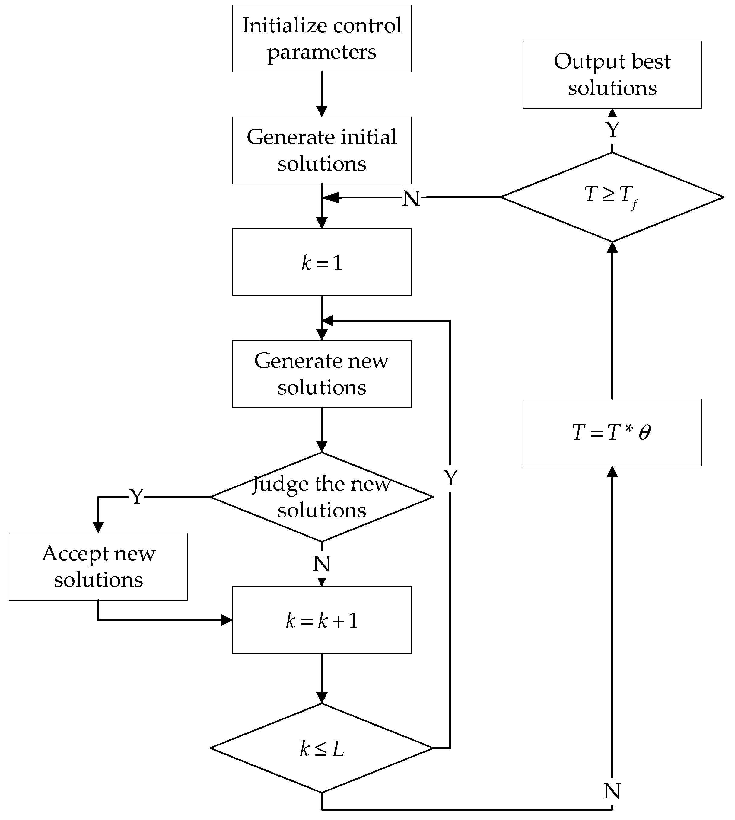
Thus, the detailed procedure of SAAH (see Figure 5) is shown as follows.

Step 1: Initialize control parameters: $T_0$, $T_f$, $\theta$, $L$ and $OF{V}_{1best}$.

Step 2: According to Constraints (4) and (5), calculate $R_n^0$.

Step 3: Randomly allocate ${\displaystyle \sum _{k=0}^{M-m}V{D}_{nmk}}$ and $V{D}_{nm}{}^{\prime }$ into blocks and satisfy Constraints (3–5), and generate the initial solutions; then calculate $OF{V}_{1current}$ and set $k=1$.

Step 4: Adjust the allocation of ${\displaystyle \sum _{k=0}^{M-m}V{D}_{nmk}}$ and $V{D}_{nm}{}^{\prime }$ according to Constraints (3–5); then generate new solutions and calculate $OF{V}_{1new}$.

Step 5: If $OF{V}_{1new}\le OF{V}_{1current}$, then set $OF{V}_{1current}=OF{V}_{1new}$ and $k=k+1$, and turn to Step 6; otherwise, calculate the probability of accepting new solutions ($p=\exp (-\frac{OF{V}_{1new}-OF{V}_{1current}}{T})$), and determine whether to accept $OF{V}_{1new}$, and set $k=k+1$ and turn to Step 7.

Step 6: If $OF{V}_{1new}\le OF{V}_{1best}$, then set $OF{V}_{1best}=OF{V}_{1new}$ and turn to Step 7.

Step 7: If $k\le L$, then turn to Step 4; otherwise, set $T=T\ast \theta$, if $T\ge T_f$, then turn to Step 3; otherwise, output $OF{V}_{1best}$.

5.2. Heuristic Algorithm Based on Rolling Horizon

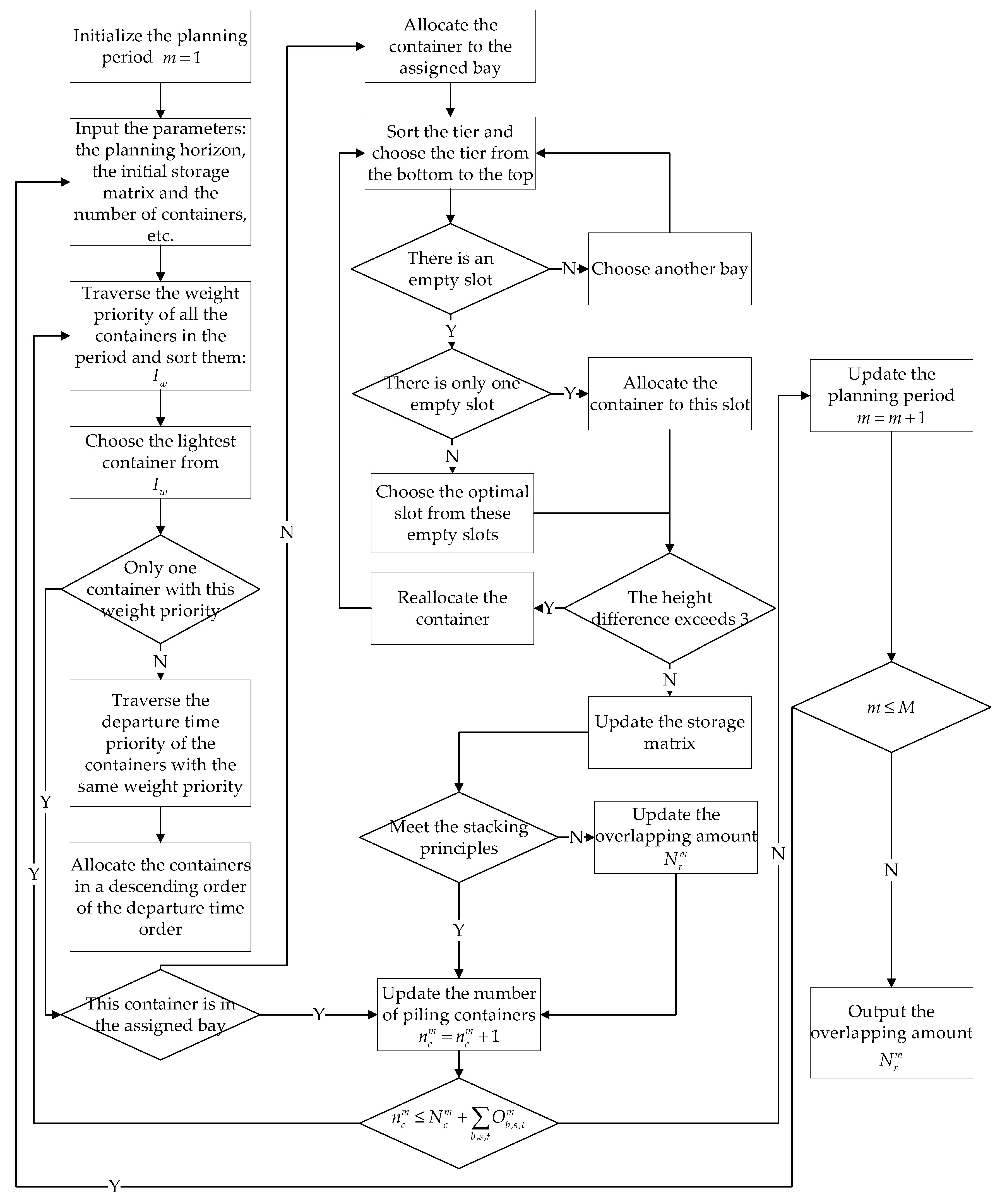
It is difficult to solve CSAP using traditional algorithms, and thus we used the HARH to solve the problem effectively and obtain an optimal solution, which is used in Reference [1].

The method used here was like Reference [1], while the difference was just that in this paper the arrival port order was not considered according to the characteristics of the proposed problem. Therefore, the detailed description of HARH is not present in the paper, and we only show the flow diagram of HARH (shown in Figure 6) and the notations used in the flow diagram.

$I_w$: the set of weight priority in an ascending order: $I_w=\{i_{w\min },\dots ,i_w,\dots ,i_{w\max }\}$; $i_w$ means the container with the specified weight priority;

$n_c^m$: the number of the container during the period $m$;

$N_r^m$: the overlapping amount.

6. Computational Experiments

In this section, some computational experiments were conducted to verify the feasibility and effectiveness of our algorithms. First, some initial settings about the experiments were proposed. Second, a small-sized experiment of one day was implemented to validate if the proposed algorithm was feasible and effective. Third, a large-sized comparison experiment of five days was carried out to validate the effectiveness of our algorithms. Fourth, a comparison experiment between different influence factors was conducted.

6.1. Initial Setting

In order to conduct the experiments, some initial settings were set up.

• All the experiments were based on the layout shown in Figure 1 and Figure 2.
• In all the experiments, we set a planning horizon to be three, a planning epoch to be one and a planning period to be six hours. Thus, one planning epoch had four planning periods, while one planning horizon had 12 planning periods.
• Following surveys made on some famous Chinese container terminals, railway container terminals and RWICTs, such as Dalian RWICT, Chengdu Railway Container Terminal, there were always three RMGCs traveling on the same railway track, which were responsible for the fixed container blocks.
• In our experiments, in order to guarantee safe and feasible stacking operations, we selected 12 blocks of ICs in the railway container yards based on the survey data and the IC blocks were equally divided by three RMGCs.
• There were five bays in each block, which had four tiers and five stacks. As a result of re-handling operations, when one bay had four tiers, it was essential to leave three empty slots in the bay. Therefore, one bay could store 17 containers at most. Therefore, the storage capacity of a block ($C_n$) was 100 and storage coefficient (${\omega }_n$) was 0.85.
• According to the pre-experiments, when the parameter of the algorithm was: T₀ = 99, T_f = 1, $\theta$ = 0.9, and L = 1200, SAAH had better effect in solving CBAP.
• All computational experiments were carried out based on a personal computer with Intel Core i7-8650U at 4.20 GHz processors and 16 GB RAM.

6.2. Small-Sized Experiments

A small-sized experiment of one day was conducted to verify the feasibility of our method. The information of inbound containers is shown in

Table 2. Number of inbound containers on vessels or inner trucks waiting for discharging and assigning to the railway container yard (VDs) in the planning period.

Container Type	m = 1	m = 2	m = 3	m = 4
${\displaystyle \sum _{n=1}^{12}V{D}_{nm}{}^{\prime }}$	240	225	236	221
${\displaystyle \sum _{n=1}^{12}{\displaystyle \sum _{k=0}^{M-m}V{D}_{nmk}}}$	440	458	436	448

and

Table 3. Number of inbound containers that have been already stored in the railway container yard, waiting for loading onto trains (TPs) in the planning period and the total number of containers in the block n before the planning period ($R_n^0$).

Container Type		n = 1	n = 2	n = 3	n = 4	n = 5	n = 6	n = 7	n = 8	n = 9	n = 10	n = 11	n = 12
$R_n^0$		50	54	45	56	55	48	57	43	46	51	42	49
$T{P}_{nm}^0$	m = 1	10	11	15	10	12	9	12	11	8	7	9	10
	m = 2	12	13	11	13	14	11	10	8	9	11	10	11
	m = 3	13	7	9	12	11	10	9	9	11	12	13	7
	m = 4	9	11	12	11	10	5	11	10	10	8	9	10

. The storage plan of each block in the planning period is shown in

Table 4. The storage plan of each block in the planning period.

Container Type		n = 1	n = 2	n = 3	n = 4	n = 5	n = 6	n = 7	n = 8	n = 9	n = 10	n = 11	n = 12
$V{D}_{nm}{}^{\prime }$	m = 1	20	20	20	20	20	20	20	20	20	20	20	20
	m = 2	19	19	19	19	19	19	19	19	19	19	19	16
	m = 3	20	20	20	20	20	20	20	20	20	20	20	16
	m = 4	18	18	18	18	18	18	18	18	18	18	18	23
${\displaystyle \sum _{k=0}^{M-m}V{D}_{nmk}}$	m = 1	37	37	37	37	37	37	37	37	37	37	37	33
	m = 2	38	38	38	38	38	38	38	38	38	38	38	40
	m = 3	36	36	36	36	36	36	36	36	36	36	36	40
	m = 4	37	37	37	37	37	37	37	37	37	37	37	41

.

In this experiment, the value of $OF{V}_1$ was 38, and the computational time in solving CBAP was 18.3 s.

Based on the computational experiment above, a comparison experiment between our method and a regular allocation algorithm (RAA) was performed to evaluate the performance of our method. RAA is a regular method for RWICTs. In RAA, container block allocation usually allocates containers to its near blocks, while container slot allocation usually allocates containers to empty slots in the storage block one after another.

The results are shown in

Table 5. The comparison experiment results between our method and regular allocation algorithm in one day.

Planning Period	$\mathbf{Our} \mathbf{Method} \mathit{O}\mathit{F}{\mathit{V}}_{1\mathit{O}\mathit{M}}$	$\mathbf{Our} \mathbf{Method} \mathit{O}\mathit{F}{\mathit{V}}_{2\mathit{O}\mathit{M}}$	$\mathbf{Regular} \mathbf{Allocation} \mathbf{Algorithm} \mathit{O}\mathit{F}{\mathit{V}}_{1\mathit{R}\mathit{A}\mathit{A}}$	$\mathbf{Regular} \mathbf{Allocation} \mathbf{Algorithm} \mathit{O}\mathit{F}{\mathit{V}}_{2\mathit{R}\mathit{A}\mathit{A}}$	$\mathit{G}\mathit{A}{\mathit{P}}_1$	$\mathit{G}\mathit{A}{\mathit{P}}_2$
m = 1	38	7	483	26	92.1%	73.0%
m = 2		11		28		60.7%
m = 3		10		27		63.0%
m = 4		16		34		52.9%

. Here we introduced $GA{P}_1$ and $GA{P}_2$ as the difference between $OF{V}_1$ and $OF{V}_2$ calculated by our method and RAA, respectively. The notations used in the calculation of $GA{P}_1$ as well as $GA{P}_2$ and the calculation of $GA{P}_1$ and $GA{P}_2$ was as follows.

$OF{V}_{1OM}$: $OF{V}_1$ calculated by our method;

$OF{V}_{1RAA}$: $OF{V}_1$ calculated by RAA;

$OF{V}_{2OM}$: $OF{V}_2$ calculated by our method;

$OF{V}_{2RAA}$: $OF{V}_2$ calculated by RAA;

$GA{P}_1$: the absolute relative difference between $OF{V}_{1OM}$ and $OF{V}_{1RAA}$;

$GA{P}_2$: the absolute relative difference between $OF{V}_{2OM}$ and $OF{V}_{2RAA}$.

The calculation of $GA{P}_1$ and $GA{P}_2$ is as follows:

$$GA{P}_1=\frac{\left|OF{V}_{1RAA}-OF{V}_{1OM}\right|}{OF{V}_{1RAA}}\ast 100\%,$$

(23)

$$GA{P}_2=\frac{\left|OF{V}_{2RAA}-OF{V}_{2OM}\right|}{OF{V}_{2RAA}}\ast 100\%.$$

(24)

It can be obviously observed that $OF{V}_{1OM}$ and $OF{V}_{2OM}$ were both fewer than $OF{V}_{1RAA}$ and $OF{V}_{2RAA}$; in the meanwhile $GA{P}_1$ and the average $GA{P}_2$ were 92.1% and 62.4%, separately. In addition, the computational time of our method and RAA in solving CBAP was 18.3 s and 25.4 s, respectively, while the average computational time of our method and RAA in solving CSAP was 20.3 s and 24.5 s, respectively.

Thus, our method was better than RAA not only in solving CBAP, but in solving CSAP. Consequently, the proposed algorithm was feasible in solving SSAP.

6.3. Large-Sized Comparison Experiments

Then a comparison experiment of five days between our method and RAA was carried out to verify the effectiveness of our method. The computational results are in

Table 6. The comparison experiment results between our method and the regular allocation algorithm (RAA) in five days.

Planning Period	$\mathbf{Our} \mathbf{Method} \mathit{O}\mathit{F}{\mathit{V}}_{1\mathit{O}\mathit{M}}$	$\mathbf{Our} \mathbf{Method} \mathit{O}\mathit{F}{\mathit{V}}_{2\mathit{O}\mathit{M}}$	$\mathbf{Regular} \mathbf{Allocation} \mathbf{Algorithm} \mathit{O}\mathit{F}{\mathit{V}}_{1\mathit{R}\mathit{A}\mathit{A}}$	$\mathbf{Regular} \mathbf{Allocation} \mathbf{Algorithm} \mathit{O}\mathit{F}{\mathit{V}}_{2\mathit{R}\mathit{A}\mathit{A}}$	$\mathit{G}\mathit{A}{\mathit{P}}_1$	$\mathit{G}\mathit{A}{\mathit{P}}_2$
m = 1	169	7	1,219	26	86.1%	73.0%
m = 2		11		28		60.7%
m = 3		10		27		63.0%
m = 4		16		34		52.9%
m = 5		12		27		55.6%
m = 6		15		37		59.4%
m = 7		12		34		64.7%
m = 8		11		33		66.7%
m = 9		20		50		60.0%
m = 10		16		46		65.2%
m = 11		15		38		60.5%
m = 12		23		58		60.3%
m = 13		19		53		64.2%
m = 14		9		33		72.7%
m = 15		8		25		68.0%
m = 16		10		33		69.7%
m = 17		13		34		61.8%
m = 18		10		30		66.7%
m = 19		9		28		67.8%
m = 20		8		26		69.2%

.

Meanwhile, as is observed from Table 5, both $OF{V}_{1RAA}$ and $OF{V}_{2RAA}$ were larger than $OF{V}_{1OM}$ and $OF{V}_{2OM}$; in the meanwhile, $GA{P}_1$ and the average $GA{P}_2$ were 86.1% and 64.1%, respectively. In addition, the computational time of our method and RAA in solving CBAP was 50.7 s and 120.8 s, separately, while the average computational time of our method and RAA in solving CSAP was 78.6 s and 130.5 s, respectively.

Therefore, our method has better performance than RAA in a large-sized problem. Therefore our method was an effective method in solving SSAP.

6.4. Comparison Experiments between Different Influence Factors

Finally, in order to compare the importance between different influence factors (the weight constraint and departure time constraint), we conducted a contrast experiment of five days. We also introduced the difference ($GA{P}_3$) between the $OF{V}_2$ with the weight constraint and departure time constraint as the important factor to evaluate the performance of HARH. The notations and calculation of $GA{P}_3$ are as follow. The results are shown in

Table 7. The results of comparison experiment between the weight and departure time constraint.

Planning Period	$\mathit{O}\mathit{F}{\mathit{V}}_{2\mathit{w}}$	$\mathit{O}\mathit{F}{\mathit{V}}_{2\mathit{e}}$	$\mathit{G}\mathit{A}{\mathit{P}}_3$
m = 1	7	9	22.2%
m = 2	11	14	21.4%
m = 3	10	12	16.7%
m = 4	16	23	30.4%
m = 5	12	17	29.4%
m = 6	15	20	25.0%
m = 7	12	19	36.8%
m = 8	11	15	26.7%
m = 9	20	26	23.0%
m = 10	16	21	23.8%
m = 11	15	20	25.0%
m = 12	23	32	28.1%
m = 13	19	28	32.1%
m = 14	9	13	30.8%
m = 15	8	13	38.5%
m = 16	10	14	28.6%
m = 17	13	19	31.6%
m = 18	10	14	28.6%
m = 19	9	12	25.0%
m = 20	8	13	38.5%

.

$OF{V}_{2w}$: $OF{V}_2$ with the weight constraint as the most important factor;

$OF{V}_{2e}$: $OF{V}_2$ with the departure time constraint as the most important factor;

$GA{P}_3$: the relative difference between $OF{V}_{2w}$ and $OF{V}_{2e}$.

$$GA{P}_3=\frac{\left|OF{V}_{2e}-OF{V}_{2w}\right|}{OF{V}_{2e}}\ast 100\%.$$

(25)

As is observed from Table 7, the values of $OF{V}_{2w}$ were all less than the values of $OF{V}_{2e}$. Therefore, when stacking containers, weight constraint was the most important impact factor of CSAP, which should be considered first.

7. Conclusion

In our paper, we introduced the storage space problem (SSAP) of inbound containers (ICs) in rail–water intermodal container terminals (RWICTs), which included the container block allocation problem (CBAP) and container slot allocation problem (CSAP). Meanwhile, not only allocation operation constraints and workload constraints but specific allocation position constraints and allocation preference constraints were considered in the proposed problem. Then a two-stage model of SSAP was formulated, whose objective was to balance the block workload and reduce the overlapping amounts. To solve the problem, we introduced a simulated annealing algorithm based on heuristic (SAAH) and improved heuristic algorithm based on rolling horizon (HARH).

Some computational experiments were conducted. The small-sized experiment verified that the proposed algorithm was feasible in solving SSAP. Then a contrast experiment of large-sized between our method and regular allocation algorithm (RAA) was conducted, and the results showed that our method was efficient to balance the distribution of ICs and reduce the overlapping amount. Finally, we also carried out a comparison experiment between different influence factors in CSAP and the result indicated that the overlapping amount in the weight constraint was less than that in the departure time constraint. Consequently, the weight constraint was the most important factor in stacking containers.

However, there were still some limitations in our paper. Firstly, we only considered inbound containers, so it is necessary to consider both inbound and outbound containers in this problem. Secondly, we did not consider the uncertain factors in our model, which will also affect SSAP. Thirdly, the scheduling of handling equipment could also have been added into our problems.

References

- Chang, Y.M.; Zhu, X.N.; Haghani, A. The outbound container slot allocation based on the stowage plan in rail–water intermodal container terminals. Meas. Control 2019. [Google Scholar] [CrossRef]
- Carlo, H.J.; Vis, I.F.A.; Roodbergen, K.J. Storage Yard Operations in Container Terminals: Literature Overview, Trends, and Research Directions. Flex. Serv. Manuf. J. 2015, 27, 224–262. [Google Scholar] [CrossRef]
- Wiese, J.; Kliewer, N.; Suhl, L. A Survey of Container Terminal Characteristics and Equipment Types. Working Paper. University of Paderborn. 2009. Available online: wiwi.unipaderborn.de/fileadmin/lehrstuehle/department-3/wiwi-dep-3-ls-5/Forschung/Publikationen/wiese_et_al_a_survey_of_container_terminal_characteristics_and_equipment_types_2009.pdf (accessed on 1 May 2012).
- Wiese, J.; Suhl, L.; Kliewer, N. Mathematical Models and Solution Methods for Optimal Container Terminal Yard Layouts. OR Spectr. 2010, 32, 427–452. [Google Scholar] [CrossRef]
- Zhang, C.; Liu, J.; Wan, Y.W.; Murty, K.G.; Linn, R.J. Storage Space Allocation in Container Terminals. Transp. Res. B-Meth. 2003, 37, 883–903. [Google Scholar] [CrossRef]
- Casey, B.; Kozan, E. Optimizing Container Storage Processes at Multimodal Terminals. J. Oper. Res. Soc. 2012, 63, 1126–1142. [Google Scholar] [CrossRef]
- Kim, K.Y.; Kim, K.H. A Routing Algorithm for A Single Transfer Crane to Load Export Containers onto A Containership. Comput. Ind. Eng. 1997, 33, 673–676. [Google Scholar] [CrossRef]
- Guo, X.; Huang, S.Y. Dynamic Space and Time Partitioning for Gantry Crane Workload Management in Container Terminals. Transp. Sci. 2012, 46, 134–148. [Google Scholar] [CrossRef]
- Lee, Y.; Lee, Y.J. A Heuristic for Retrieving Container from A Yard. Comput. Oper. Res. 2010, 37, 1139–1147. [Google Scholar] [CrossRef]
- Huang, S.H.; Lin, T.H. Heuristic Algorithms for Container Pre-marshalling Problems. Comput. Ind. Eng. 2012, 62, 13–20. [Google Scholar] [CrossRef]
- Kim, K.H.; Park, Y.M.; Ryu, K.R. Deriving Decision Rules to Locate Export Containers in Container Yards. Eur. J. Oper. Res. 2000, 124, 89–101. [Google Scholar] [CrossRef]
- Kim, K.H.; Kang, T.P. A Note on a Dynamic Space-allocation Method for Outbound Containers. Eur. J. Oper. Res. 2003, 148, 92–101. [Google Scholar] [CrossRef]
- Yan, X.; Zhao, N.; Bian, Z.; Mi, C. An Intelligent Storage Determining Method for Inbound Containers in Container Terminals. J. Coast. Res. 2005, 73, 197–204. [Google Scholar]
- Lee, L.H.; Chew, E.P.; Tan, K.C.; Han, Y. An Optimization Model for Storage Yard Management in Transshipment Hubs. OR Spectr. 2006, 28, 107–129. [Google Scholar] [CrossRef]
- Mckendall, A.R.; Jaramillo, J.R. A Tabu Search Heuristic for the Dynamic Space Allocation Problem. Comput. Oper. Res. 2006, 33, 768–789. [Google Scholar] [CrossRef]
- Mckendall, A.R. Improved Tabu Search Heuristics for the Dynamic Space Allocation Problem. Comput. Oper. Res. 2008, 35, 3347–3359. [Google Scholar] [CrossRef]
- Bazzazi, M.; Safaei, N.; Javadian, N. A Genetic Algorithm to Solve the Storage Space Allocation Problem in A Container Terminal. Comput. Ind. Eng. 2009, 56, 44–52. [Google Scholar] [CrossRef]
- Choe, R.; Park, T.; Oh, M.S.; Kang, J.; Ryu, K.R. Generating A Rehandling-free Intra-block Remarshaling Plan for An Automated Container Yard. J. Intell. Manuf. 2011, 22, 201–217. [Google Scholar] [CrossRef]
- Yu, M.; Qi, X. Storage Space Allocation Models for Inbound Containers in An Automatic Container Terminal. Eur. J. Oper. Res. 2013, 226, 32–45. [Google Scholar] [CrossRef]
- Sharif, O.; Huynh, N. Storage Space Allocation at Marine Container Terminals Using Ant-based Control. Expert Syst. Appl. 2013, 40, 2323–2330. [Google Scholar] [CrossRef]
- Jiang, X.; Chew, E.P.; Lee, L.H.; Tan, K.C. Short-term Space Allocation for Storage Yard Management in A Transshipment Hub Port. OR Spectr. 2014, 36, 879–901. [Google Scholar] [CrossRef]
- Zheng, H.X.; Du, L.; Dong, J. Optimization Model on Container Slot Allocation in Container Yard with Mixed Storage Mode. J. Transp. Syst. Eng. Inf. Technol. 2012, 12, 153–159. [Google Scholar]
- Wang, L.; Zhu, X.N.; Yan, W.; Xie, Z.Y.; Li, Q.B. Optimization Model of Mixed Storage in Railway Container Terminal Yard. J. Transp. Syst. Eng. Inf. Technol. 2013, 13, 172–178. [Google Scholar]
- Wang, L.; Zhu, X.N.; Xie, Z.Y. Storage Space Allocation of Inbound Container in Railway Container Terminal. Math. Probl. Eng. 2014, 2014. [Google Scholar] [CrossRef]
- Liu, C.J.; Hu, Z.H. Space Allocation Optimization Model and Algorithm for Outbound Containers in the Yard. J. Jiangsu Univ. Sci. Technol. (Nat. Sci. Ed.) 2016, 30, 490–497. [Google Scholar]
- Ji, M.J.; Huang, S.J.; Guo, W.W. Container Allocation Optimization of the Center Terminal Yard under Rail-sea Intermodal Transportation. Syst. Eng. Theory Pract. 2016, 36, 1555–1567. [Google Scholar]
- Li, Y.J.; Zhu, X.N.; Wang, L.; Chen, X. Stowage Plan Based Slot Optimal Allocation in Rail-Water Container Terminal. J. Control Sci. Eng. 2017, 2017. [Google Scholar] [CrossRef]
Figure 1.
The schematic diagram of the railway container yard in a rail–water intermodal container terminals (RWICTs).
Figure 2.
The schematic diagram of a block.
Figure 3.
An example of the rolling planning horizon.
Figure 4.
An example of overlapping amount calculation.
Figure 5.
The flow diagram of the simulated annealing algorithm based on heuristics (SAAH).
Figure 6.
The flow diagram of the heuristic algorithm based on a rolling horizon (HARH).