Group Decision-Making Based on the VIKOR Method with Trapezoidal Bipolar Fuzzy Information

Abstract

The VIKOR methodology stands out as an important multi-criteria decision-making technique. VIKOR stands for “VIekriterijumsko KOmpromisno Rangiranje”, a Serbian term for “multi-criteria optimization and compromise solution”. It has been adapted to sources of information with sundry formats. We contribute to that strand on literature with a design of a new multiple-attribute group decision-making method called the trapezoidal bipolar fuzzy VIKOR method. It consists of a suitable redesign of the VIKOR approach so that it can use information with bipolar configurations. Bipolar fuzzy sets (and numbers) establish a symmetrical trade-off between two judgmental constituents of human thinking. The agents acquire uncertain and vague information in the form of linguistic variables parameterized by trapezoidal bipolar fuzzy numbers. Trapezoidal bipolar fuzzy numbers are considered by decision-makers for assigning the preference information of alternatives with respect to different attributes. Our non-trivial adaptation necessitates several steps. The ranking function of bipolar fuzzy numbers is employed to make a simple decision matrix with real numbers as its entries. Shannon’s entropy concept is applied to evaluate the normalized weights for attributes that may be either partially or completely unknown to the decision-makers. The ordering of the alternatives is obtained by assorting the maximum group utility and the individual regret of the opponent in an ascending manner. For illustration, the proposed technique is applied to two group decision-making problems, namely, the selection of waste treatment methods and the site to plant a thermal power station. A comparison of this method with the trapezoidal bipolar fuzzy TOPSIS method is also presented.

1. Introduction

Decision-making is a procedure of selecting or classifying an alternative or an action from a set of feasible or possible actions with respect to different factors depending on the choice of decision-makers. The most important factors for any decision are the source of information, collection of alternatives, preference values, and the environment in which the decision is made. The decision-making process becomes quite complicated when it involves the multiplicity of criteria or constraints. Thus, a multi-attribute decision-making (MADM) method indicates the results on the basis of conflicting criteria, such as cost-type and benefit-type criteria. There are many real-life problems that are solved on the basis of multiple criteria. These multi-criteria decision-making (MCDM) problems may adopt a complex form when a group of different decision-makers is involved for making decisions, and this technique is known as multi-criteria group decision-making (MCGDM). There is a wide range of MADM methods to determine the solution of MCDM problems in many disciplines, including business management, information technology, economics, social sciences, diagnosis, and so forth. The advancement in MADM methods is closely associated to the development of computer technology, which has made it simpler and easier to deal with complex, complicated, and large amounts of information or data.

In the last few decades, a number of MADM methods and their different invariants or versions, such as simple additive weighting (SAW) [1], the analytic hierarchy process (AHP) [2], VIekriterijumsko KOmpromisno Rangiranje, or the multi-criteria optimization and compromise solution (VIKOR) [3], Technique for the Order of Preference by Similarity to an Ideal Solution (TOPSIS) [4], Preference Ranking Organization Method for Enrichment of Evaluations (PROMETHEE) [5], Elimination and Choice Translating Reality (ELECTRE) [6], and grey system theory [7] have been introduced to find the solution for a set of actions depending on conflicting criteria. However, there are many real-world problems with imprecise and uncertain information for which the classical MADM methods are not helpful. So, in 1970, Bellman and Zadeh [8] first initiated the idea of fuzzy MADM methods to deal with vague and ambiguous data. Since then, decision-making with the fuzzy set theory has become a most common and interesting research area for researchers and practitioners. In the VIKOR method, the solution is obtained by combining the maximum group utility and individual regret of the opponent in the form of a compromise solution which directs the decision-makers to the final result. For example, Opricovic [9] provided the compromise solution of water resources planning using the VIKOR method, and Chang and Hsu [10] used the modified version of the VIKOR method to find the classification of land subdivision according to watershed vulnerability. El-Santawy [11] solved a personnel training selection problem using the VIKOR method. Furthermore, Opricovic [12] gave the comparison of an extended VIKOR with other outranking methods. Sanayei et al. [13] presented the VIKOR model using fuzzy information for group decision-making problems of supplier selection. Shemshadi et al. [14] developed a fuzzy VIKOR technique for the selection of suppliers in which he used the concept of an entropy measure to determine the objective weights of attributes [15,16]. Kim and Chung [17] proposed a fuzzy VIKOR method for evaluating the vulnerability of water supply to climate change and variability in South Korea. Luo and Wang [18] also presented the intuitionistic version of an extender VIKOR method for multi-attribute decision-making using a new concept of distance measuring. YinYang bipolar fuzzy sets (bipolar fuzzy sets) were presented by Zhang [19,20] as an extension of fuzzy sets [21] in order to deal with the bipolar judgmental components of human reasoning. On the basis of bipolar fuzzy sets, the bipolar fuzzy linguistic variables and bipolar fuzzy numbers were proposed by Akram and Arshad [22]. Alghamdi et al. [23] developed the multi-criteria decision-making method under a bipolar fuzzy environment. In this context, TOPSIS and ELECTRE-I have been adapted and then applied to diagnosis by Akram et al. [24]. Recently, Samanta and Sarkar [25] presented a study on generalized fuzzy graphs as a useful representation for the analysis of things such as social networks or competition in ecosystems. Generalized fuzzy trees are another interesting contribution with related purposes [26].

The VIKOR method was proposed by Opricovic in 1998 for multi-attribute optimization of a complex system. The method focuses on the compromise ranking list, the compromise solution, and the interval of the strategy weight for the preference solution. It is based on the multi-criteria ranking index, which gives the measure of closeness to the ideal solution. The VIKOR method was developed on the basis of the following form of the $L_p$-metric:

$$L_{p,k}={\left\{\underset{j=1}{\sum ^n}{\left[w_j\left(f_j^{*}-f_{kj}\right)/\left(f_j^{*}-f_j^{-}\right)\right]}^p\right\}}^{1/p},1\le p\le \infty ;k=1,2,\cdots ,n.$$

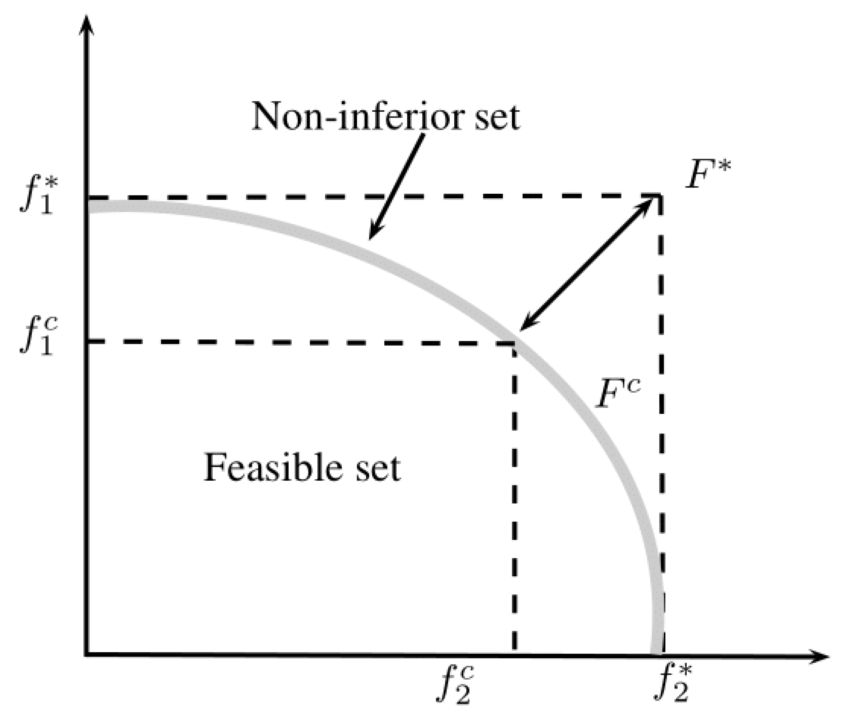
Within the VIKOR method, $L_{1,k}$ and $L_{\infty ,k}$ are used to formulate the ranking measure. The solution is obtained by maximum group utility (or majority rule) and minimum individual regret of the opponent by considering the minimum values of ranking lists. The compromise solution $F^c$ is a feasible solution which is closest to the ideal solution $F^{*}$, and “compromise” means an agreement which is established by mutual concession, as illustrated in Figure 1.

Different versions of the VIKOR method can be effectively used and applied to obtain the compromise solution when the information is given in the form of crisp or fuzzy values. There are many MCDM problems which have bipolar information (that captures the double-sided or bipolar information of human reasoning or knowledge), and at present they cannot be solved by using the VIKOR strategy that consists of achieving a compromise solution. To overcome this difficulty, in this paper we present a new version of the VIKOR method that accounts for the concept of YinYang bipolar fuzzy sets. A bipolar fuzzy set is an efficient tool which can be used to handle double-sided information or bipolar reasoning. To position our analysis, the contribution of different authors towards the study of VIKOR-type methods and bipolar data has been given in

Table 1. Contribution of different authors towards the VIKOR method and bipolar information.

Authors	Year	Contributions
Zhang [19]	1994	Initiated the concept of bipolar fuzzy sets.
Opricovic, Tzeng [3]	1998	Introduce the VIKOR method.
Opricovic, Tzeng [12]	2007	Extended VIKOR method in comparison with outranking method.
Sanayei et al. [13]	2010	Introduce the fuzzy VIKOR method for group decision-making.
Shemshadi et al. [14]	2011	Application of fuzzy VIKOR using entropy weight information.
Luo, Wang [18]	2017	Present an intuitionistic fuzzy VIKOR method.
Akram, Arshad [22]	2019	Introduce the bipolar fuzzy numbers.
Shumaiza et al.	This paper	Present the trapezoidal bipolar fuzzy VIKOR method.

. In this research study, we propose a VIKOR method by using bipolar fuzzy linguistic variables which are further parameterized by trapezoidal bipolar fuzzy numbers [22]. We compute the normalized weights of attributes by employing Shannon’s entropy concept of weight-measuring information [14]. We construct a simple decision matrix for further processing by applying the ranking function of bipolar fuzzy numbers given in [22]. We compute the majority rule and the individual regret of the opponent to find the ordering of alternatives. We explain the proposed method with the help of two numerical problems. We also provide a comparison of the VIKOR method with TOPSIS using trapezoidal bipolar fuzzy numbers.

The outline of this paper is as follows: Section 2 contains the preliminary concepts; Section 3 introduces the trapezoidal bipolar fuzzy VIKOR method; Section 4 provides numerical examples; Section 5 contains the comparison of the aforementioned method with TOPSIS for trapezoidal bipolar fuzzy numbers; and Section 6 concludes this paper.

2. Preliminaries

YinYang bipolar fuzzy sets are defined as follows:

Definition 1.

[19] Let U be a non-empty universe of discourse. A bipolar fuzzy set $\tilde{\mathcal{B}}$ on U is defined as

$$\tilde{\mathcal{B}}=\left\{(u,{\lambda }_{\tilde{\mathcal{B}}}^{+}\left(u\right),{\lambda }_{\tilde{\mathcal{B}}}^{-}\left(u\right))\mid u\in U\right\},$$

where ${\lambda }_{\tilde{\mathcal{B}}}^{+}\left(u\right):U\to [0,1]$ and ${\lambda }_{\tilde{\mathcal{B}}}^{-}\left(u\right):U\to [-1,0]$ represent the satisfaction and dissatisfaction degrees of the bipolar fuzzy set $\tilde{\mathcal{B}}$, respectively.

In particular, we can use bipolar fuzzy numbers in the following way:

Definition 2.

[22] A bipolar fuzzy number $\tilde{\mathcal{B}}$ is a bipolar fuzzy subset defined on the real line $\mathbb{R}$, having the form

$$\tilde{\mathcal{B}}=〈V,W〉=〈[{\nu }_1,{\nu }_2,{\nu }_3,{\nu }_4],[{\omega }_1,{\omega }_2,{\omega }_3,{\omega }_4]〉,$$

such that the satisfaction degree ${\lambda }_{\tilde{\mathcal{B}}}^{+}\left(u\right)$ of $\tilde{\mathcal{B}}$ is defined as

$${\lambda }_{\tilde{\mathcal{B}}}^{+}\left(u\right)=\left\{\begin{array}{cc}{\lambda }_{\tilde{\mathcal{B}}}^{l+}\left(u\right),\hfill & \mathit{if}u\in [{\nu }_1,{\nu }_2],\hfill \\ 1,\hfill & \mathit{if}u\in [{\nu }_2,{\nu }_3],\hfill \\ {\lambda }_{\tilde{\mathcal{B}}}^{r+}\left(u\right),\hfill & \mathit{if}u\in [{\nu }_3,{\nu }_4],\hfill \\ 0,\hfill & \mathit{otherwise},\hfill \end{array}\right.$$

and the dissatisfaction degree ${\lambda }_{\tilde{\mathcal{B}}}^{-}\left(u\right)$ of $\tilde{\mathcal{B}}$ is defined as

$${\lambda }_{\tilde{\mathcal{B}}}^{-}\left(u\right)=\left\{\begin{array}{cc}{\lambda }_{\tilde{\mathcal{B}}}^{l-}\left(u\right),\hfill & \mathit{if}u\in [{\omega }_1,{\omega }_2],\hfill \\ 1,\hfill & \mathit{if}u\in [{\omega }_2,{\omega }_3],\hfill \\ {\lambda }_{\tilde{\mathcal{B}}}^{r-}\left(u\right),\hfill & \mathit{if}u\in [{\omega }_3,{\omega }_4],\hfill \\ 0,\hfill & \mathit{otherwise},\hfill \end{array}\right.$$

where ${\lambda }_{\tilde{\mathcal{B}}}^{l+}\left(u\right):[{\nu }_1,{\nu }_2]\to [0,1]$ and ${\lambda }_{\tilde{\mathcal{B}}}^{r+}\left(u\right):[{\nu }_3,{\nu }_4]\to [0,1]$ represent the left and right membership degrees of ${\lambda }_{\tilde{\mathcal{B}}}^{+}\left(u\right)$, respectively. Similarly, ${\lambda }_{\tilde{\mathcal{B}}}^{l-}\left(u\right):[{\omega }_1,{\omega }_2]\to [-1,0]$ and ${\lambda }_{\tilde{\mathcal{B}}}^{r-}\left(u\right):[{\omega }_3,{\omega }_4]\to [-1,0]$ represent the left and right membership degrees of ${\lambda }_{\tilde{\mathcal{B}}}^{-}\left(u\right)$, respectively.

Just as trapezoidal fuzzy numbers are a remarkable and useful type of fuzzy number [27], bipolar fuzzy numbers are especially easy for manipulations when they have the following form:

Definition 3.

[22] A bipolar fuzzy number $\tilde{\mathcal{B}}=〈V,W〉=〈[{\nu }_1,{\nu }_2,{\nu }_3,{\nu }_4],[{\omega }_1,{\omega }_2,{\omega }_3,{\omega }_4]〉$ is known as the trapezoidal bipolar fuzzy number, denoted by $〈({\nu }_1,{\nu }_2,{\nu }_3,{\nu }_4),({\omega }_1,{\omega }_2,{\omega }_3,{\omega }_4)〉$, if its satisfaction and dissatisfaction degrees are as follows:

$${\lambda }_{\tilde{\mathcal{B}}}^{+}\left(u\right)=\left\{\begin{array}{cc}\frac{u-{\nu }_1}{{\nu }_2-{\nu }_1},\hfill & \mathit{if}u\in [{\nu }_1,{\nu }_2],\hfill \\ 1,\hfill & \mathit{if}u\in [{\nu }_2,{\nu }_3],\hfill \\ \frac{{\nu }_4-u}{{\nu }_4-{\nu }_3},\hfill & \mathit{if}u\in [{\nu }_3,{\nu }_4],\hfill \\ 0,\hfill & \mathit{otherwise},\hfill \end{array}\right.$$

and

$${\lambda }_{\tilde{\mathcal{B}}}^{-}\left(u\right)=\left\{\begin{array}{cc}\frac{-(u-{\omega }_1)}{{\omega }_2-{\omega }_1},\hfill & \mathit{if}u\in [{\omega }_1,{\omega }_2],\hfill \\ -1,\hfill & \mathit{if}u\in [{\omega }_2,{\omega }_3],\hfill \\ \frac{-({\omega }_4-u)}{{\omega }_4-{\omega }_3},\hfill & \mathit{if}u\in [{\omega }_3,{\omega }_4],\hfill \\ 0,\hfill & \mathit{otherwise}.\hfill \end{array}\right.$$

Definition 4.

[22] Consider a trapezoidal bipolar fuzzy number $\tilde{\mathcal{B}}=〈({\nu }_1,{\nu }_2,{\nu }_3,{\nu }_4),({\omega }_1,{\omega }_2,{\omega }_3,{\omega }_4)〉$. Then, it can be converted into a crisp real number by using the ranking function, as follows:

$$\left(m\left(V\right)+\left[\frac{-{\nu }_1-{\nu }_2+{\nu }_3+{\nu }_4}{2}\right]\right)-\left(m\left(W\right)+\left[\frac{-{\omega }_1-{\omega }_2+{\omega }_3+{\omega }_4}{2}\right]\right),$$

where $m\left(V\right)=\frac{{\nu }_1+{\nu }_2+{\nu }_3+{\nu }_4}{4}$ and $m\left(W\right)=\frac{{\omega }_1+{\omega }_2+{\omega }_3+{\omega }_4}{4}$ are the mean values of respective sets.

3. Trapezoidal Bipolar Fuzzy VIKOR Method

In this section, a multi-attribute decision-analysis (MADA) approach, based on the VIKOR method combined with trapezoidal bipolar fuzzy numbers is presented to solve multi-criteria decision-making problems, and named as the trapezoidal bipolar fuzzy VIKOR method. The procedure of this method inaugurates as follows: define the problem area and choose an appropriate or relevant decision-making group; identify the linguistic variables and define their corresponding values; consider a set of criteria to evaluate the alternatives; construct a decision matrix; determine the normalized weights by the entropy weight method [14]; find out the best and worst values which are used to compute the maximum group utility and the individual regret of the opponent; and order the alternatives and find a compromise solution.

Consider a multi-attribute decision-making problem consisting of a set of m feasible alternatives ${\mathcal{T}}_{\alpha },\alpha =1,2,\cdots ,m$, which are assessed by k decision-makers ${\mathbb{D}}_{\gamma },\gamma =1,2,\cdots ,k$, on the basis of n conflicting and non-commensurable criteria ${\mathcal{K}}_{\beta },\beta =1,2,\cdots ,n$. The performance ratings of each alternative ${\mathcal{T}}_{\alpha }$ with respect to each criterion ${\mathcal{K}}_{\beta }$ by decision-maker ${\mathbb{D}}_{\gamma }$ construct a decision matrix denoted by $T={\left[t_{\alpha \beta }^{\gamma }\right]}_{m\times n}$. The step-by-step procedure of the trapezoidal bipolar fuzzy VIKOR method is explained as follows:

3.1. Identification of Linguistic Variables

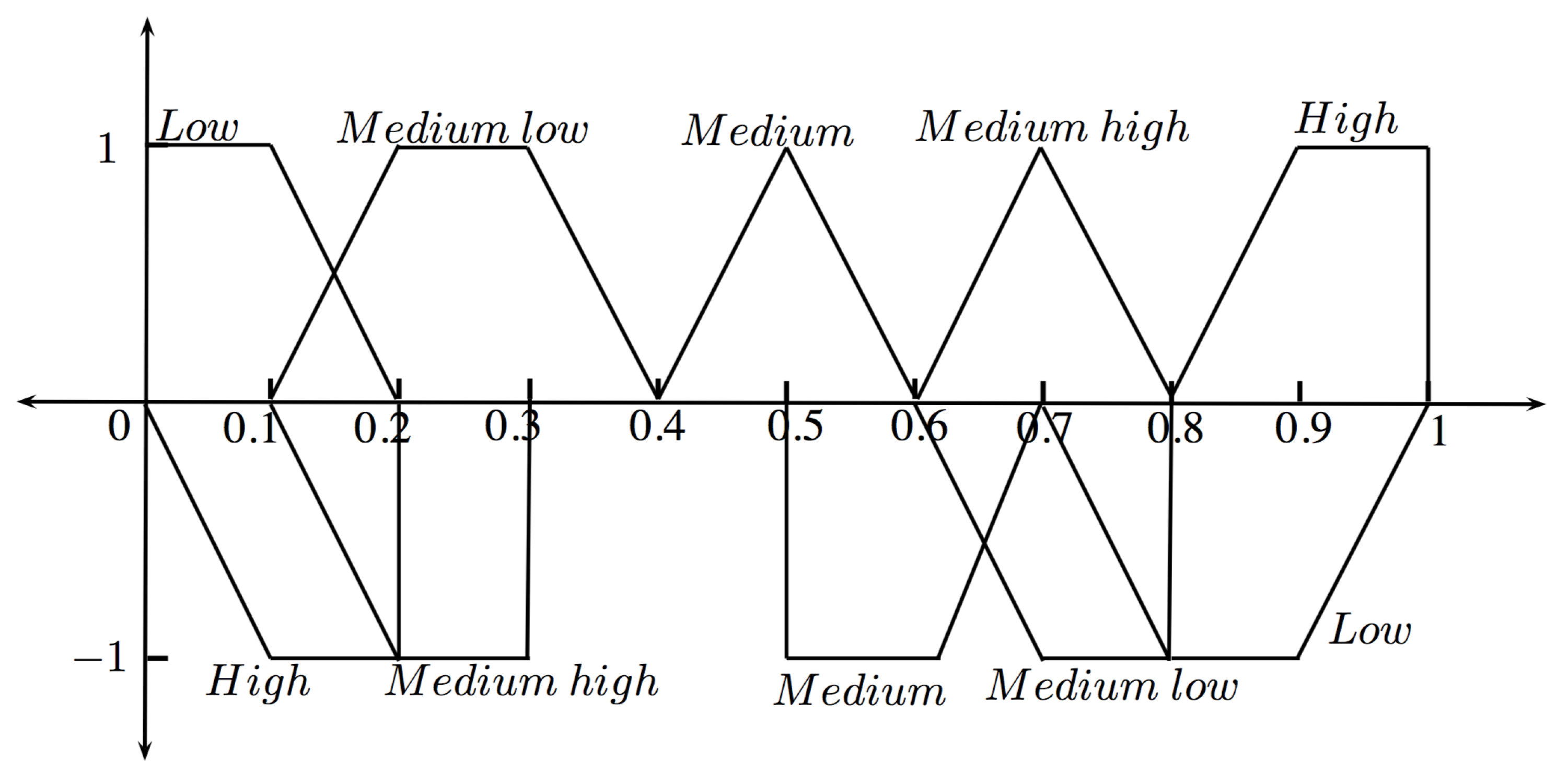
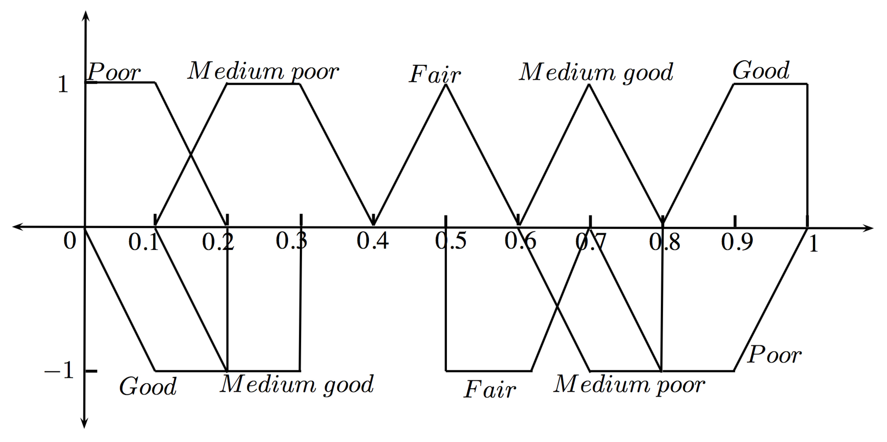
Identify and define the appropriate linguistic variables and their corresponding membership values to estimate the ratings of alternatives with respect to criteria. Two sets of suitable linguistic variables in the form of trapezoidal bipolar fuzzy numbers are used for the assessment of bipolar fuzzy ratings of cost and benefit criteria given by decision-makers, shown in Figure 2 and Figure 3, respectively. The values of trapezoidal bipolar fuzzy numbers are considered within the numerical domain $[0,1]$.

3.2. Construction of Decision Matrix

Suppose that there are m alternatives ${\mathcal{T}}_{\alpha }$ which are assessed on the basis of n criteria ${\mathcal{K}}_{\beta }$ evaluated by each decision-maker ${\mathbb{D}}_{\gamma }$ (for $\gamma =1,\dots ,k$), and the rating values corresponding to the linguistic variables are expressed in the form of k decision matrices, as follows:

$$T={\left[t_{\alpha \beta }^{\gamma }\right]}_{m\times n}=\left[\begin{array}{cccc}{t}_{11}^{\gamma }& t_{12}^{\gamma }& \cdots & t_{1n}^{\gamma }\\ t_{21}^{\gamma }& t_{22}^{\gamma }& \cdots & t_{2n}^{\gamma }\\ .& .& .& .\\ .& .& .& .\\ .& .& .& .\\ t_{m1}^{\gamma }& t_{m2}^{\gamma }& \dots & t_{mn}^{\gamma }\end{array}\right] \mathrm{for} \mathrm{each} \gamma =1,\dots ,k,$$

where $t_{\alpha \beta }^{\gamma }=〈[{\nu }_{\alpha \beta 1}^{\gamma },{\nu }_{\alpha \beta 2}^{\gamma },{\nu }_{\alpha \beta 3}^{\gamma },{\nu }_{\alpha \beta 4}^{\gamma }],[{\omega }_{\alpha \beta 1}^{\gamma },{\omega }_{\alpha \beta 2}^{\gamma },{\omega }_{\alpha \beta 3}^{\gamma },{\omega }_{\alpha \beta 4}^{\gamma }]〉,\alpha =1,2,\cdots ,m,\beta =1,2,\cdots ,n,$ $\gamma =1,2,\cdots ,k,$ is a trapezoidal bipolar fuzzy number. The aggregated bipolar fuzzy rating of each alternative evaluated by criteria ${\mathcal{K}}_{\beta }$ and denoted by $t_{\alpha \beta }$ = $\langle [{\nu }_{\alpha \beta 1},{\nu }_{\alpha \beta 2},{\nu }_{\alpha \beta 3},{\nu }_{\alpha \beta 4}]$, $[{\omega }_{\alpha \beta 1},{\omega }_{\alpha \beta 2},{\omega }_{\alpha \beta 3},{\omega }_{\alpha \beta 4}]\rangle$, is computed in the following manner:

$$\begin{array}{c}\hfill \left\{\begin{array}{c}{\nu }_{\alpha \beta 1}={\displaystyle \underset{\gamma }{min}}\left\{{\nu }_{\alpha \beta 1}^{\gamma }\right\},\hfill \\ {\nu }_{\alpha \beta 2}=\frac{1}{\gamma }{\displaystyle \underset{\gamma =1}{\sum ^k}}{\nu }_{\alpha \beta 2}^{\gamma },\hfill \\ {\nu }_{\alpha \beta 3}=\frac{1}{\gamma }{\displaystyle \underset{\gamma =1}{\sum ^k}}{\nu }_{\alpha \beta 3}^{\gamma },\hfill \\ {\nu }_{\alpha \beta 4}={\displaystyle \underset{\gamma }{max}}\left\{{\nu }_{\alpha \beta 4}^{\gamma }\right\},\hfill \end{array}\right.\hspace{1em}\mathrm{and}\hspace{1em}\left\{\begin{array}{c}{\omega }_{\alpha \beta 1}={\displaystyle \underset{\gamma }{min}}\left\{{\omega }_{\alpha \beta 1}^{\gamma }\right\},\hfill \\ {\omega }_{\alpha \beta 2}=\frac{1}{\gamma }{\displaystyle \underset{\gamma =1}{\sum ^k}}{\omega }_{\alpha \beta 2}^{\gamma },\hfill \\ {\omega }_{\alpha \beta 3}=\frac{1}{\gamma }{\displaystyle \underset{\gamma =1}{\sum ^k}}{\omega }_{\alpha \beta 3}^{\gamma },\hfill \\ {\omega }_{\alpha \beta 4}={\displaystyle \underset{\gamma }{max}}\left\{{\omega }_{\alpha \beta 4}^{\gamma }\right\}.\hfill \end{array}\right.\end{array}$$

(1)

Thus, the aggregated bipolar fuzzy decision matrix is constructed as,

$$T={\left[t_{\alpha \beta }\right]}_{m\times n}=\left[\begin{array}{cccc}{t}_{11}& t_{12}& \cdots & t_{1n}\\ t_{21}& t_{22}& \cdots & t_{2n}\\ .& .& .& .\\ .& .& .& .\\ .& .& .& .\\ t_{m1}& t_{m2}& \dots & t_{mn}\end{array}\right].$$

3.3. Ranking of Bipolar Fuzzy Numbers

Then, the bipolar fuzzy numbers are converted into crisp values of real numbers by using the ranking function, as follows:

$$\begin{array}{c}\hfill \begin{array}{cc}\hfill f_{\alpha \beta }=& \left(\left[\frac{{\nu }_{\alpha \beta 1}+{\nu }_{\alpha \beta 2}+{\nu }_{\alpha \beta 3}+{\nu }_{\alpha \beta 4}}{4}\right]+\left[\frac{-{\nu }_{\alpha \beta 1}-{\nu }_{\alpha \beta 2}+{\nu }_{\alpha \beta 3}+{\nu }_{\alpha \beta 4}}{2}\right]\right)-\hfill \\ \hfill & \left(\left[\frac{{\omega }_{\alpha \beta 1}+{\omega }_{\alpha \beta 2}+{\omega }_{\alpha \beta 3}+{\omega }_{\alpha \beta 4}}{4}\right]+\left[\frac{-{\omega }_{\alpha \beta 1}-{\omega }_{\alpha \beta 2}+{\omega }_{\alpha \beta 3}+{\omega }_{\alpha \beta 4}}{2}\right]\right),\hfill \end{array}\end{array}$$

(2)

and construct a simple decision matrix $F=\left\{f_{\alpha \beta }\right\}$ for further calculations.

3.4. Calculating the Normalized Weights

To calculate the important weights of the conflicting criteria ${\mathcal{K}}_{\beta }$ by the entropy weight information method, we firstly need to find out the projection value of each criteria, denoted by ${\mathbb{P}}_{\alpha \beta }$, using the following formula:

$${\mathbb{P}}_{\alpha \beta }=\frac{f_{\alpha \beta }}{{\displaystyle \underset{\alpha =1}{\sum ^m}}{f}_{\alpha \beta }}.$$

(3)

After the projection values, entropy values are computed by using the following expression,

$${\mathbb{E}}_{\beta }=-c\underset{\alpha =1}{\sum ^m}{\mathbb{P}}_{\alpha \beta }log\left({\mathbb{P}}_{\alpha \beta }\right),$$

(4)

where $c={(log\left(m\right))}^{-1}$ is a constant. By using these entropy values, the degree of divergence ${\mathrm{d}}_{\beta }$ for each criteria is calculated as

$${\mathrm{d}}_{\beta }=1-{\mathbb{E}}_{\beta },\beta =1,2,\cdots ,n.$$

(5)

The divergence value ${\mathrm{d}}_{\beta }$ represents the inherent contrast intensity of criteria ${\mathcal{K}}_{\beta }$. As in the case of entropy, it is an absolute (not relative) magnitude. The higher the value of ${\mathrm{d}}_{\beta }$, the more important the criterion ${\mathcal{K}}_{\beta }$ is for the problem. Then, the weights for each criteria are obtained as

$${\mathrm{W}}_{\beta }=\frac{{\mathrm{d}}_{\beta }}{{\displaystyle \underset{\beta =1}{\sum ^n}}{\mathrm{d}}_{\beta }}.$$

(6)

3.5. Finding the Best and Worst Value

In this subsection, the best value $f_{\beta }^{*}$ and the worst value $f_{\beta }^{-}$ are determined for all criteria ${\mathcal{K}}_{\beta }$ according to whether they are benefit or cost criteria. A set of benefit-type criteria is denoted by $J^b$, and the set of cost-type criteria is denoted by $J^c$, which are calculated as

$$\begin{array}{cc}\hfill f_{\beta }^{*}=\underset{\alpha }{max}\left\{f_{\alpha \beta }\right\},& f_{\beta }^{-}=\underset{\alpha }{min}\left\{f_{\alpha \beta }\right\},\mathrm{for}\beta \in J^b,\end{array}$$

(7)

$$\begin{array}{cc}\hfill f_{\beta }^{*}=\underset{\alpha }{min}\left\{f_{\alpha \beta }\right\},& f_{\beta }^{-}=\underset{\alpha }{max}\left\{f_{\alpha \beta }\right\},\mathrm{for}\beta \in J^c.\end{array}$$

(8)

3.6. Computing the Values ${\mathcal{S}}_{\alpha }$, ${\mathcal{R}}_{\alpha }$ and ${\mathcal{Q}}_{\alpha }$

The values of maximum group utility or the majority rule ${\mathcal{S}}_{\alpha }$ and the minimum individual regret of the opponent ${\mathcal{R}}_{\alpha }$ are obtained as follows:

$$\begin{array}{ccc}\hfill {\mathcal{S}}_{\alpha }& =& \underset{\beta =1}{\sum ^n}{\mathrm{W}}_{\beta }\frac{f_{\beta }^{*}-f_{\alpha \beta }}{f_{\beta }^{*}-f_{\beta }^{-}},\hfill \end{array}$$

(9)

$$\begin{array}{ccc}\hfill {\mathcal{R}}_{\alpha }& =& \underset{\beta }{max}\left({\mathrm{W}}_{\beta }\frac{f_{\beta }^{*}-f_{\alpha \beta }}{f_{\beta }^{*}-f_{\beta }^{-}}\right).\hfill \end{array}$$

(10)

Afterward, the value of ${\mathcal{Q}}_{\alpha }$ can be calculated by using the formula

$${\mathcal{Q}}_{\alpha }=\upsilon \frac{{\mathcal{S}}_{\alpha }-{\mathcal{S}}^{*}}{{\mathcal{S}}^{-}-{\mathcal{S}}^{*}}+(1-\upsilon )\frac{{\mathcal{R}}_{\alpha }-{\mathcal{R}}^{*}}{{\mathcal{R}}^{-}-{\mathcal{R}}^{*}},$$

(11)

where ${\mathcal{S}}^{*}={\displaystyle \underset{\alpha }{min}}\left\{{\mathcal{S}}_{\alpha }\right\}$, ${\mathcal{S}}^{-}={\displaystyle \underset{\alpha }{max}}\left\{{\mathcal{S}}_{\alpha }\right\}$, ${\mathcal{R}}^{*}={\displaystyle \underset{\alpha }{min}}\left\{{\mathcal{R}}_{\alpha }\right\}$ and ${\mathcal{R}}^{-}={\displaystyle \underset{\alpha }{max}}\left\{{\mathcal{R}}_{\alpha }\right\}$. $\upsilon$ is known as the weight of the strategy of the majority of the criteria, and its value lies in interval $[0,1].$

3.7. Ordering the Alternatives

The alternatives are ordered by sorting the values of ${\mathcal{S}}_{\alpha }$, ${\mathcal{R}}_{\alpha }$, and ${\mathcal{Q}}_{\alpha }$ in an ascending order. As a result, we have three ranking lists according to the crisp values of $\mathcal{S}$, $\mathcal{R}$, and $\mathcal{Q}$, which are further utilized to propose the compromise solution of alternatives. The term ${\mathcal{Q}}_{\alpha }$ is the separation measure of ${\mathcal{T}}_{\alpha }$ from the best alternative, which implies that the smaller value of $\mathcal{Q}$ indicates the better alternative.

3.8. Compromising the Solution

In this step, a compromise solution of the alternative ${\mathcal{T}}^{\left(1\right)}$ is determined, which is the best-ranked solution by the measure $\mathcal{Q}$ (minimum) if it satisfies the following two conditions:

$\mathbb{C}1.$ “Acceptable advantage”

$$\mathcal{Q}\left({\mathcal{T}}^{\left(2\right)}\right)-\mathcal{Q}\left({\mathcal{T}}^{\left(1\right)}\right)\ge \mathcal{DQ},$$

where ${\mathcal{T}}^{\left(2\right)}$ is the second-positioned alternative in the ordering list of $\mathcal{Q}$ and $\mathcal{DQ}=\frac{1}{m-1}$, and m is the number of favorable or considered alternatives.

$\mathbb{C}2.$ “Acceptable stability in decision-making”

According to this condition, the alternative ${\mathcal{T}}^{\left(1\right)}$, which is best-ranked by $\mathcal{Q},$ must also be the best-ranked by $\mathcal{S}$ or/and $\mathcal{R}$.

If any one of the above-mentioned conditions is not satisfied, then a set of compromise solutions is obtained as follows:

$\mathbb{CS}1.$ If only the condition $\mathbb{C}2$ is not satisfied, then the set of compromise solutions consists of the alternatives ${\mathcal{T}}^{\left(1\right)}$ and ${\mathcal{T}}^{\left(m\right)}$.

$\mathbb{CS}2.$ If the condition $\mathbb{C}1$ is not satisfied, then this compromise solution contains the alternatives ${\mathcal{T}}^{\left(1\right)},{\mathcal{T}}^{\left(2\right)},\cdots ,{\mathcal{T}}^{\left(M\right)};{\mathcal{T}}^{\left(M\right)}$ is obtained by the relation $\mathcal{Q}\left({\mathcal{T}}^{\left(M\right)}\right)-\mathcal{Q}\left({\mathcal{T}}^{\left(1\right)}\right)\ge \mathcal{DQ}$ for maximum M.

4. Numerical Example

In this section, we are going to explain two real-world problems as applications of the proposed method, which has been described in the previous section, to show the reliability of this method.

4.1. Selection of Health-Care Waste Treatment Strategy

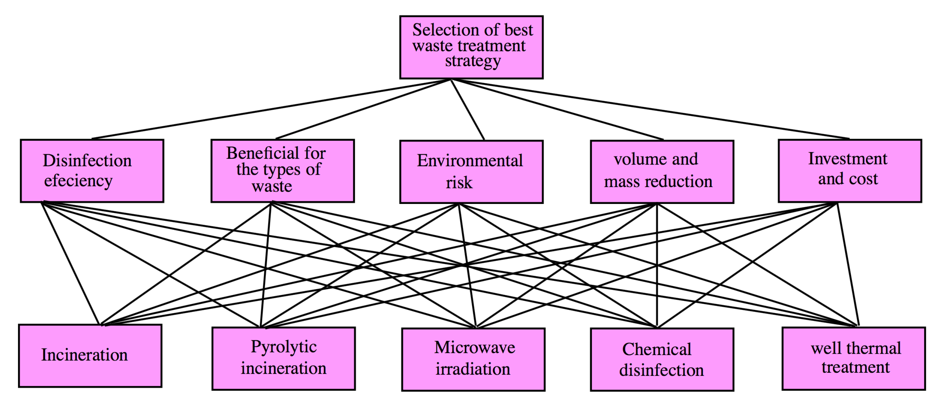
Health-care waste treatment organization is a high-priority environmental, public, and health concern in developing countries. These organizations work on destructing waste materials, and to do so, use different waste treatment strategies, such as incineration, steam sterilization, Rotary kiln, Pyrolytic incineration, single-chamber incineration, wet thermal treatment, microwave irradiations, and landfill processes. Assuming that health-care management has to select a waste treatment method to decompose waste minerals and other chemical or pharmaceutical infectious waste, after initial screening, the management will select five well-known methods for further evaluation that include ${\mathcal{T}}_1=$ Incineration, ${\mathcal{T}}_2=$ Pyrolytic incineration, ${\mathcal{T}}_3=$ Microwave irradiation, ${\mathcal{T}}_4=$ Chemical disinfection, and ${\mathcal{T}}_5=$ Wet thermal treatment. A group of three decision-makers is decided upon to evaluate these five alternatives on the basis of five conflicting criteria, such as ${\mathcal{K}}_1=$ Disinfection efficiency, ${\mathcal{K}}_2=$ Beneficial for the types of waste, ${\mathcal{K}}_3=$ Environmental risk, ${\mathcal{K}}_4=$ Volume and mass reduction, and ${\mathcal{K}}_5=$ Investment and cost. ${\mathcal{K}}_1,{\mathcal{K}}_2$ and ${\mathcal{K}}_4$ are benefit criteria, whereas ${\mathcal{K}}_3$ and ${\mathcal{K}}_5$ are considered as cost criteria. The framework for evaluating the waste treatment strategy is provided in Figure 4.

Step 1.

The group of decision-makers choose the linguistic variables to be assessed in the performance ratings of alternatives with respect to the criteria given in Figure 2 and Figure 3. The linguistic variables and their corresponding trapezoidal bipolar fuzzy numbers are presented for cost-type criteria and benefit-type criteria in

Table 2. Linguistic variables and values for cost-type criteria.

Linguistic Variable	Abbreviation	Bipolar Fuzzy Number
$Low$	L	$\langle (0.0,0.0,0.1,0.2),(0.7,0.8,0.9,1.0)\rangle$
$Mediumlow$	$ML$	$\langle (0.1,0.2,0.3,0.4),(0.6,0.7,0.8,0.8)\rangle$
$Medium$	M	$\langle (0.4,0.5,0.5,0.6),(0.5,0.5,0.6,0.7)\rangle$
$Mediumhigh$	$MH$	$\langle (0.6,0.7,0.7,0.8),(0.1,0.2,0.3,0.3)\rangle$
$High$	H	$\langle (0.8,0.9,1.0,1.0),(0.0,0.1,0.2,0.2)\rangle$

and

Table 3. Linguistic variables and values for benefit-type criteria.

Linguistic Variable	Abbreviation	Bipolar Fuzzy Number
$Poor$	P	$\langle (0.0,0.0,0.1,0.2),(0.7,0.8,0.9,1.0)\rangle$
$MediumPoor$	$MP$	$\langle (0.1,0.2,0.3,0.4),(0.6,0.7,0.8,0.8)\rangle$
$Fair$	F	$\langle (0.4,0.5,0.5,0.6),(0.5,0.5,0.6,0.7)\rangle$
$Mediumgood$	$MG$	$\langle (0.6,0.7,0.7,0.8),(0.1,0.2,0.3,0.3)\rangle$
$Good$	G	$\langle (0.8,0.9,1.0,1.0),(0.0,0.1,0.2,0.2)\rangle$

, respectively.

Step 2.

These linguistic terms are used by decision-makers to determine the performance ratings of alternatives with respect to the conflicting criteria, which are shown in

Table 4. Performance ratings by decision-makers (linguistic terms).

	${\mathbb{D}}_1$					${\mathbb{D}}_2$					${\mathbb{D}}_3$
	${\mathcal{T}}_{\mathbf{1}}$	${\mathcal{T}}_{\mathbf{2}}$	${\mathcal{T}}_{\mathbf{3}}$	${\mathcal{T}}_{\mathbf{4}}$	${\mathcal{T}}_{\mathbf{5}}$	${\mathcal{T}}_{\mathbf{1}}$	${\mathcal{T}}_{\mathbf{2}}$	${\mathcal{T}}_{\mathbf{3}}$	${\mathcal{T}}_{\mathbf{4}}$	${\mathcal{T}}_{\mathbf{5}}$	${\mathcal{T}}_{\mathbf{1}}$	${\mathcal{T}}_{\mathbf{2}}$	${\mathcal{T}}_{\mathbf{3}}$	${\mathcal{T}}_{\mathbf{4}}$	${\mathcal{T}}_{\mathbf{5}}$
${\mathcal{K}}_1$	$MG$	G	G	$MG$	$MG$	G	F	$MG$	F	$MG$	$MG$	G	F	$MG$	$MG$
${\mathcal{K}}_2$	F	G	F	$MG$	$MG$	F	G	$MG$	G	F	$MG$	G	G	$MG$	F
${\mathcal{K}}_3$	M	$MG$	H	$MH$	M	$MH$	M	M	H	$MG$	M	M	H	H	M
${\mathcal{K}}_4$	G	G	F	$MG$	$MG$	$MG$	G	F	G	$MG$	G	$MG$	G	G	$MG$
${\mathcal{K}}_5$	$MH$	H	$MH$	H	M	$ML$	M	H	$MH$	$MH$	$MH$	M	$MH$	$MH$	$MH$

.

These linguistic variables are then converted into corresponding trapezoidal bipolar fuzzy numbers given in Table 2 and Table 3, and the results are shown in

Table 5. Performance ratings by decision-makers (bipolar fuzzy numbers).

		${\mathcal{K}}_1$	${\mathcal{K}}_2$	${\mathcal{K}}_3$	${\mathcal{K}}_4$	${\mathcal{K}}_5$
${\mathbb{D}}_1$	${\mathcal{T}}_1$	$\langle (0.6,0.7,0.7,0.8),$	$\langle (0.4,0.5,0.5,0.6),$	$\langle (0.4,0.5,0.5,0.6),$	$\langle (0.8,0.9,1.0,1.0),$	$\langle (0.6,0.7,0.7,0.8),$
		$(0.1,0.2,0.3,0.3)\rangle$	$(0.5,0.5,0.6,0.7)\rangle$	$(0.5,0.5,0.6,0.7)\rangle$	$(0.0,0.1,0.2,0.2)\rangle$	$(0.1,0.2,0.3,0.3)\rangle$
	${\mathcal{T}}_2$	$\langle (0.8,0.9,1.0,1.0),$	$\langle (0.8,0.9,1.0,1.0),$	$\langle (0.6,0.7,0.7,0.8),$	$\langle (0.8,0.9,1.0,1.0),$	$\langle (0.8,0.9,1.0,1.0),$
		$(0.0,0.1,0.2,0.2)\rangle$	$(0.0,0.1,0.2,0.2)\rangle$	$(0.1,0.2,0.3,0.3)\rangle$	$(0.0,0.1,0.2,0.2)\rangle$	$(0.0,0.1,0.2,0.2)\rangle$
	${\mathcal{T}}_3$	$\langle (0.8,0.9,1.0,1.0),$	$\langle (0.4,0.5,0.5,0.6),$	$\langle (0.8,0.9,1.0,1.0),$	$\langle (0.4,0.5,0.5,0.6),$	$\langle (0.6,0.7,0.7,0.8),$
		$(0.0,0.1,0.2,0.2)\rangle$	$(0.5,0.5,0.6,0.7)\rangle$	$(0.0,0.1,0.2,0.2)\rangle$	$(0.5,0.5,0.6,0.7)\rangle$	$(0.1,0.2,0.3,0.3)\rangle$
	${\mathcal{T}}_4$	$\langle (0.6,0.7,0.7,0.8),$	$\langle (0.6,0.7,0.7,0.8),$	$\langle (0.6,0.7,0.7,0.8),$	$\langle (0.6,0.7,0.7,0.8),$	$\langle (0.8,0.9,1.0,1.0),$
		$(0.1,0.2,0.3,0.3)\rangle$	$(0.1,0.2,0.3,0.3)\rangle$	$(0.1,0.2,0.3,0.3)\rangle$	$(0.1,0.2,0.3,0.3)\rangle$	$(0.0,0.1,0.2,0.2)\rangle$
	${\mathcal{T}}_5$	$\langle (0.6,0.7,0.7,0.8),$	$\langle (0.6,0.7,0.7,0.8),$	$\langle (0.4,0.5,0.5,0.6),$	$\langle (0.6,0.7,0.7,0.8),$	$\langle (0.4,0.5,0.5,0.6),$
		$(0.1,0.2,0.3,0.3)\rangle$	$(0.1,0.2,0.3,0.3)\rangle$	$(0.5,0.5,0.6,0.7)\rangle$	$(0.1,0.2,0.3,0.3)\rangle$	$(0.5,0.5,0.6,0.7)\rangle$
${\mathbb{D}}_2$	${\mathcal{T}}_1$	$\langle (0.8,0.9,1.0,1.0),$	$\langle (0.4,0.5,0.5,0.6),$	$\langle (0.6,0.7,0.7,0.8),$	$\langle (0.6,0.7,0.7,0.8),$	$\langle (0.1,0.2,0.3,0.4),$
		$(0.0,0.1,0.2,0.2)\rangle$	$(0.5,0.5,0.6,0.7)\rangle$	$(0.1,0.2,0.3,0.3)\rangle$	$(0.1,0.2,0.3,0.3)\rangle$	$(0.6,0.7,0.8,0.8)\rangle$
	${\mathcal{T}}_2$	$\langle (0.4,0.5,0.5,0.6),$	$\langle (0.8,0.9,1.0,1.0),$	$\langle (0.4,0.5,0.5,0.6),$	$\langle (0.8,0.9,1.0,1.0),$	$\langle (0.4,0.5,0.5,0.6),$
		$(0.5,0.5,0.6,0.7)\rangle$	$(0.0,0.1,0.2,0.2)\rangle$	$(0.5,0.5,0.6,0.7)\rangle$	$(0.0,0.1,0.2,0.2)\rangle$	$(0.5,0.5,0.6,0.7)\rangle$
	${\mathcal{T}}_3$	$\langle (0.6,0.7,0.7,0.8),$	$\langle (0.6,0.7,0.7,0.8),$	$\langle (0.4,0.5,0.5,0.6),$	$\langle (0.4,0.5,0.5,0.6),$	$\langle (0.8,0.9,1.0,1.0),$
		$(0.1,0.2,0.3,0.3)\rangle$	$(0.1,0.2,0.3,0.3)\rangle$	$(0.5,0.5,0.6,0.7)\rangle$	$(0.5,0.5,0.6,0.7)\rangle$	$(0.0,0.1,0.2,0.2)\rangle$
	${\mathcal{T}}_4$	$\langle (0.4,0.5,0.5,0.6),$	$\langle (0.8,0.9,1.0,1.0),$	$\langle \left(\right(0.8,0.9,1.0,1.0),$	$\langle (0.8,0.9,1.0,1.0),$	$\langle (0.6,0.7,0.7,0.8),$
		$(0.5,0.5,0.6,0.7)\rangle$	$(0.0,0.1,0.2,0.2)\rangle$	$(0.0,0.1,0.2,0.2)\rangle$	$(0.0,0.1,0.2,0.2)\rangle$	$(0.1,0.2,0.3,0.3)\rangle$
	${\mathcal{T}}_5$	$\langle (0.6,0.7,0.7,0.8),$	$\langle (0.4,0.5,0.5,0.6),$	$\langle (0.6,0.7,0.7,0.8),$	$\langle (0.6,0.7,0.7,0.8),$	$\langle (0.6,0.7,0.7,0.8),$
		$(0.1,0.2,0.3,0.3)\rangle$	$(0.5,0.5,0.6,0.7)\rangle$	$(0.1,0.2,0.3,0.3)\rangle$	$(0.1,0.2,0.3,0.3)\rangle$	$(0.1,0.2,0.3,0.3)\rangle$
${\mathbb{D}}_3$	${\mathcal{T}}_1$	$\langle (0.6,0.7,0.7,0.8),$	$\langle (0.6,0.7,0.7,0.8),$	$\langle (0.4,0.5,0.5,0.6),$	$\langle (0.8,0.9,1.0,1.0),$	$\langle (0.6,0.7,0.7,0.8),$
		$(0.1,0.2,0.3,0.3)\rangle$	$(0.1,0.2,0.3,0.3)\rangle$	$(0.5,0.5,0.6,0.7)\rangle$	$(0.0,0.1,0.2,0.2)\rangle$	$(0.1,0.2,0.3,0.3)\rangle$
	${\mathcal{T}}_2$	$\langle (0.8,0.9,1.0,1.0),$	$\langle (0.8,0.9,1.0,1.0),$	$\langle (0.4,0.5,0.5,0.6),$	$\langle (0.6,0.7,0.7,0.8),$	$\langle (0.4,0.5,0.5,0.6),$
		$(0.0,0.1,0.2,0.2)\rangle$	$(0.0,0.1,0.2,0.2)\rangle$	$(0.5,0.5,0.6,0.7)\rangle$	$(0.1,0.2,0.3,0.3)\rangle$	$(0.5,0.5,0.6,0.7)\rangle$
	${\mathcal{T}}_3$	$\langle (0.4,0.5,0.5,0.6),$	$\langle (0.8,0.9,1.0,1.0),$	$\langle (0.8,0.9,1.0,1.0),$	$\langle (0.6,0.7,0.7,0.8),$	$\langle (0.1,0.2,0.3,0.4),$
		$(0.5,0.5,0.6,0.7)\rangle$	$(0.0,0.1,0.2,0.2)\rangle$	$(0.0,0.1,0.2,0.2)\rangle$	$(0.1,0.2,0.3,0.3)\rangle$	$(0.6,0.7,0.8,0.8)\rangle$
	${\mathcal{T}}_4$	$\langle (0.6,0.7,0.7,0.8),$	$\langle (0.6,0.7,0.7,0.8),$	$\langle (0.8,0.9,1.0,1.0),$	$\langle (0.8,0.9,1.0,1.0),$	$\langle (0.6,0.7,0.7,0.8),$
		$(0.1,0.2,0.3,0.3)\rangle$	$(0.1,0.2,0.3,0.3)\rangle$	$(0.0,0.1,0.2,0.2)\rangle$	$(0.0,0.1,0.2,0.2)\rangle$	$(0.1,0.2,0.3,0.3)\rangle$
	${\mathcal{T}}_5$	$\langle (0.6,0.7,0.7,0.8),$	$\langle (0.4,0.5,0.5,0.6),$	$\langle (0.4,0.5,0.5,0.6),$	$\langle (0.6,0.7,0.7,0.8),$	$\langle (0.6,0.7,0.7,0.8),$
		$(0.1,0.2,0.3,0.3)\rangle$	$(0.5,0.5,0.6,0.7)\rangle$	$(0.5,0.5,0.6,0.7)\rangle$	$(0.1,0.2,0.3,0.3)\rangle$	$(0.1,0.2,0.3,0.3)\rangle$

. By using these trapezoidal bipolar fuzzy numbers, an aggregated decision matrix is constructed by employing the expressions given in Equation (1), and shown in

Table 6. Aggregated decision matrix.

	${\mathcal{K}}_1$	${\mathcal{K}}_2$	${\mathcal{K}}_3$	${\mathcal{K}}_4$	${\mathcal{K}}_5$
${\mathcal{T}}_1$	$\langle (0.6,0.77,0.80,1.0),$	$\langle (0.4,0.57,0.57,0.8),$	$\langle (0.4,0.57,0.57,0.8),$	$\langle (0.6,0.83,0.9,1.0),$	$\langle (0.1,0.53,0.57,0.8),$
	$(0.0,0.17,0.27,0.3)\rangle$	$(0.1,0.4,0.5,0.7)\rangle$	$(0.1,0.4,0.5,0.7)\rangle$	$(0.0,0.13,0.23,0.3)\rangle$	$(0.1,0.37,0.47,0.8)\rangle$
${\mathcal{T}}_2$	$\langle (0.4,0.77,0.83,1.0),$	$\langle (0.8,0.9,1.0,1.0),$	$\langle (0.4,0.57,0.57,0.8),$	$\langle (0.6,0.83,0.9,1.0),$	$\langle (0.4,0.63,0.67,1.0),$
	$(0.0,0.23,0.33,0.7)\rangle$	$(0.0,0.1,0.2,0.2)\rangle$	$(0.1,0.4,0.5,0.7)\rangle$	$(0.0,0.13,0.23,0.3)\rangle$	$(0.0,0.37,0.47,0.7)\rangle$
${\mathcal{T}}_3$	$\langle (0.4,0.7,0.73,1.0),$	$\langle (0.4,0.7,0.73,1.0),$	$\langle (0.4,0.77,0.83,1.0),$	$\langle (0.4,0.57,0.57,0.8),$	$\langle (0.1,0.6,0.67,1.0),$
	$(0.0,0.27,0.37,0.7)\rangle$	$(0.0,0.27,0.37,0.7)\rangle$	$(0.0,0.23,0.33,0.7)\rangle$	$(0.1,0.4,0.5,0.7)\rangle$	$(0.0,0.33,0.43,0.8)\rangle$
${\mathcal{T}}_4$	$\langle (0.4,0.63,0.63,0.8),$	$\langle (0.6,0.77,0.8,1.0),$	$\langle (0.6,0.83,0.9,1.0),$	$\langle (0.6,0.83,0.9,1.0),$	$\langle (0.6,0.77,0.8,1.0),$
	$(0.1,0.3,0.4,0.7)\rangle$	$(0.0,0.17,0.27,0.3)\rangle$	$(0.0,0.13,0.23,0.3)\rangle$	$(0.0,0.13,0.23,0.3)\rangle$	$(0.0,0.17,0.27,0.3)\rangle$
${\mathcal{T}}_5$	$\langle (0.6,0.7,0.7,0.8),$	$\langle (0.4,0.57,0.57,0.8),$	$\langle (0.4,0.57,0.57,0.8),$	$\langle (0.6,0.7,0.7,0.8),$	$\langle (0.4,0.63,0.63,0.8),$
	$(0.1,0.2,0.3,0.3)\rangle$	$(0.1,0.4,0.5,0.7)\rangle$	$(0.1,0.4,0.5,0.7)\rangle$	$(0.1,0.2,0.3,0.3)\rangle$	$(0.1,0.3,0.4,0.7)\rangle$

.

For instance, the aggregated performance ratings of alternative ${\mathcal{T}}_1$ with respect to the criterion ${\mathcal{K}}_1$ is computed as:

$$\begin{array}{cccc}\hfill min(0.6,0.8,0.6)=0.6,& \frac{1}{3}[0.7+0.9+0.7]=0.77,\hfill & \hfill \frac{1}{3}[0.7+1.0+0.7]=0.80,& max(0.8,1.0,0.8)=1.0,\hfill \\ \hfill min(0.1,0.0,0.1)=0.0,& \frac{1}{3}[0.2+0.1+0.2]=0.17,\hfill & \hfill \frac{1}{3}[0.3+0.2+0.3]=0.27,& max(0.3,0.2,0.3)=0.3.\hfill \end{array}$$

Step 3.

The aggregated bipolar fuzzy decision matrix is then converted into a simple decision matrix consisting of crisp values as entries by deploying the ranking function given in Equation (2) The decision matrix F is given in

Table 7. Decision matrix F.

F	${\mathcal{K}}_1$	${\mathcal{K}}_2$	${\mathcal{K}}_3$	${\mathcal{K}}_4$	${\mathcal{K}}_5$
${\mathcal{T}}_1$	$0.62$	$0.01$	$0.01$	$0.70$	$0.04$
${\mathcal{T}}_2$	$0.37$	$0.80$	$0.01$	$0.70$	$0.21$
${\mathcal{T}}_3$	$0.29$	$0.29$	$0.37$	$0.01$	$0.24$
${\mathcal{T}}_4$	$0.09$	$0.60$	$0.70$	$0.70$	$0.62$
${\mathcal{T}}_5$	$0.43$	$0.01$	$0.01$	$0.43$	$0.09$

. For example, $f_{11}$ is calculated as,

$$\begin{array}{cc}\hfill f_{11}& =\left(\left[\frac{0.6+0.77+0.8+1}{4}\right]+\left[\frac{-0.6-0.77+0.8+1}{2}\right]\right)-\left(\left[\frac{0+0.17+0.27+0.3}{4}\right]+\left[\frac{-0-0.17+0.27+0.3}{2}\right]\right)\hfill \\ \hfill & =(0.793+0.215)-(0.185+0.2)=0.62.\hfill \end{array}$$

Step 4.

The normalized weights for the criteria are calculated in this step by applying the entropy measure information. The projection values of the criteria are computed by using Equation (3), and the results are given in

Table 8. Projection values of criteria.

${\mathbb{P}}_{\mathit{\alpha }\mathit{\beta }}$	${\mathcal{K}}_1$	${\mathcal{K}}_2$	${\mathcal{K}}_3$	${\mathcal{K}}_4$	${\mathcal{K}}_5$
${\mathcal{T}}_1$	$0.34$	$0.01$	$0.01$	$0.28$	$0.03$
${\mathcal{T}}_2$	$0.21$	$0.46$	$0.01$	$0.28$	$0.18$
${\mathcal{T}}_3$	$0.16$	$0.17$	$0.34$	$0.003$	$0.2$
${\mathcal{T}}_4$	$0.05$	$0.35$	$0.64$	$0.28$	$0.52$
${\mathcal{T}}_5$	$0.24$	$0.01$	$0.01$	$0.17$	$0.08$

. For example, ${\mathbb{P}}_{11}$ is calculated as

$$\begin{array}{c}\hfill {\mathbb{P}}_{11}=\frac{0.62}{0.62+0.37+0.29+0.09+0.43}=0.34.\end{array}$$

These projection values are then used to enumerate the entropy value and the degree of divergence for criteria using Equations (4) and (5). Furthermore, the weight for each criterion is calculated by deploying the Equation (6), and results are respectively shown in

Table 9. Entropy value, divergence, and weights of criteria.

	${\mathcal{K}}_1$	${\mathcal{K}}_2$	${\mathcal{K}}_3$	${\mathcal{K}}_4$	${\mathcal{K}}_5$
${\mathbb{E}}_{\beta }$	$0.92$	$0.69$	$0.49$	$0.86$	$0.79$
${\mathrm{d}}_{\beta }$	$0.08$	$0.31$	$0.51$	$0.14$	$0.21$
${\mathrm{W}}_{\beta }$	$0.064$	$0.248$	$0.408$	$0.112$	$0.168$

. For instance, ${\mathbb{E}}_1$, ${\mathrm{d}}_1$, and ${\mathrm{W}}_1$ are calculated here, respectively, as

$$\begin{array}{cc}{\mathbb{E}}_1\hfill & =-\frac{1}{log\left(5\right)}[0.34log\left(0.34\right)+0.21log\left(0.21\right)+0.16log\left(0.16\right)+0.05log\left(0.05\right)+0.24log\left(0.24\right)]\hfill \\ \hfill & =-\frac{1}{0.6989}(-0.6428)=0.92.\hfill \\ {\mathrm{d}}_1\hfill & =1-0.92=0.08.\hfill \\ {\mathrm{W}}_1\hfill & =\frac{0.08}{0.08+0.31+0.51+0.14+0.21}=\frac{0.08}{1.25}=0.064.\hfill \end{array}$$

Step 5.

The best or ideal value $f_{\beta }^{*}$, as well as the worst or nadir value $f_{\beta }^{-}$, for cost-type and benefit-type criteria are determined by using Equations (7) and (8), respectively, and the results are shown in

Table 10. Values $f_{\beta }^{*}$ and $f_{\beta }^{-}$.

	${\mathcal{K}}_1$	${\mathcal{K}}_2$	${\mathcal{K}}_3$	${\mathcal{K}}_4$	${\mathcal{K}}_5$
$f_{\beta }^{*}$	$0.62$	$0.80$	$0.01$	$0.70$	$0.04$
$f_{\beta }^{-}$	$0.09$	$0.01$	$0.70$	$0.01$	$0.62$

.

Step 6.

The values of ${\mathcal{S}}_{\alpha }$, ${\mathcal{R}}_{\alpha }$, and ${\mathcal{Q}}_{\alpha }$ are given in

Table 11. Values of ${\mathcal{S}}_{\alpha }$, ${\mathcal{R}}_{\alpha }$, and ${\mathcal{Q}}_{\alpha }$.

	${\mathcal{S}}_{\mathit{\alpha }}$	${\mathcal{R}}_{\mathit{\alpha }}$	${\mathcal{Q}}_{\mathit{\alpha }}$
${\mathcal{T}}_1$	$0.248$	$0.249$	$0.423$
${\mathcal{T}}_2$	$0.079$	$0.049$	$0.0$
${\mathcal{T}}_3$	$0.583$	$0.213$	$0.646$
${\mathcal{T}}_4$	$0.703$	$0.408$	$1.0$
${\mathcal{T}}_5$	$0.329$	$0.248$	$0.488$

. Here, the value of the weight of the strategy “$\upsilon$” is 0.5.

Step 7.

The ranking of waste treatment strategies according to the ascending orders of ${\mathcal{S}}_{\alpha }$, ${\mathcal{R}}_{\alpha }$, and ${\mathcal{Q}}_{\alpha }$ is shown in

Table 12. The ranking of alternatives by ${\mathcal{S}}_{\alpha }$, ${\mathcal{R}}_{\alpha }$, and ${\mathcal{Q}}_{\alpha }$.

	1	2	3	4	5
By ${\mathcal{S}}_{\alpha }$	${\mathcal{T}}_2$	${\mathcal{T}}_1$	${\mathcal{T}}_5$	${\mathcal{T}}_3$	${\mathcal{T}}_4$
By ${\mathcal{R}}_{\alpha }$	${\mathcal{T}}_2$	${\mathcal{T}}_3$	${\mathcal{T}}_5$	${\mathcal{T}}_1$	${\mathcal{T}}_4$
By ${\mathcal{Q}}_{\alpha }$	${\mathcal{T}}_2$	${\mathcal{T}}_1$	${\mathcal{T}}_5$	${\mathcal{T}}_3$	${\mathcal{T}}_4$

.

Step 8.

The two conditions mentioned in Section 3.8 are satisfied, and thus the alternative ${\mathcal{T}}_2$, that is, Pyrolytic incineration, is the best possible waste treatment strategy.

4.2. Selection of Site for Thermal Power Station

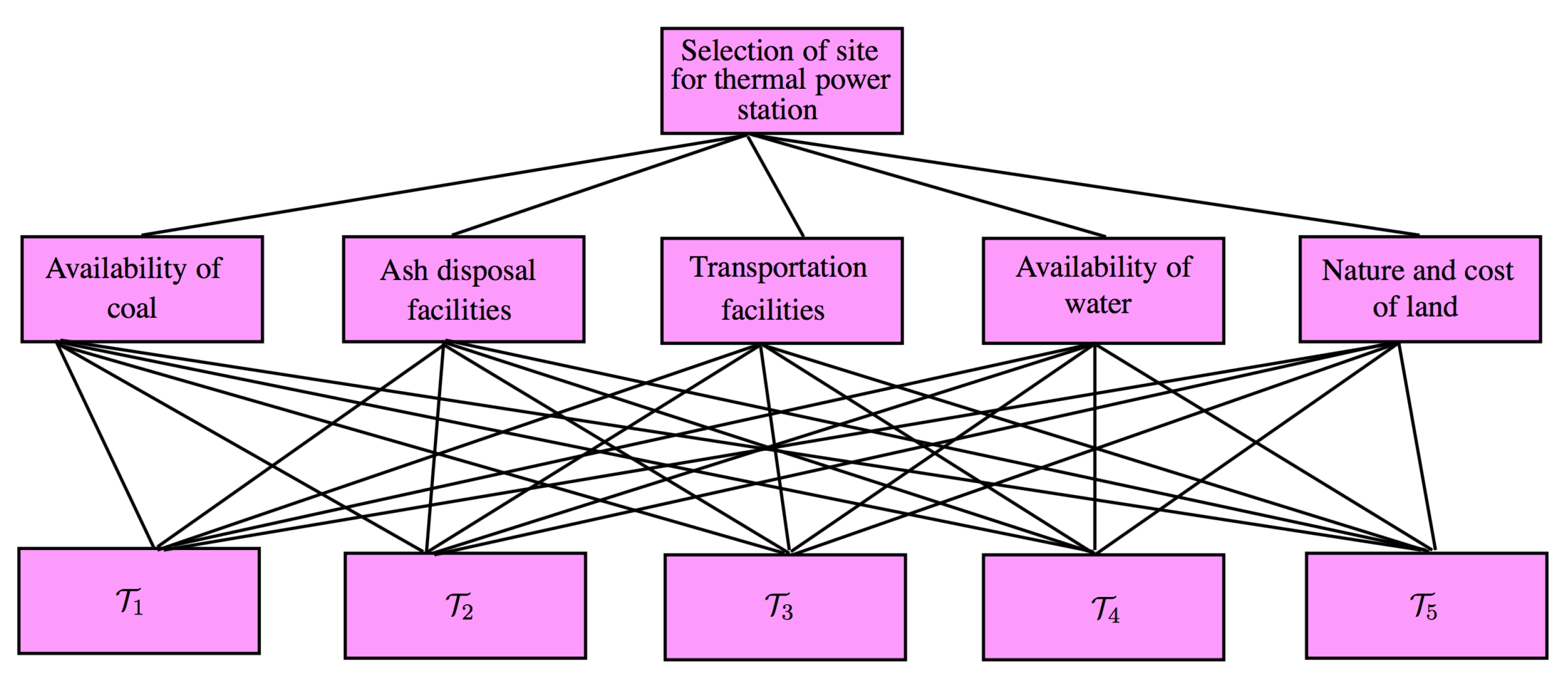
A thermal power station is a power station which converts heat energy into electrical energy by means of coal combustion. It is most important to choose a site for a thermal power station, as it needs a huge capacity of land and position to bear the static and dynamic pressure during the whole process. Suppose that the government wants to plant a thermal power station to meet the requirements of electric power. After the initial survey, five locations, such as ${\mathcal{T}}_1,{\mathcal{T}}_2,{\mathcal{T}}_3,{\mathcal{T}}_4$, and ${\mathcal{T}}_5$, are chosen for further assessment. A group of three decision-makers is appointed to examine these locations on the basis of a set of five criteria, including ${\mathcal{K}}_1=$ Availability of coal, ${\mathcal{K}}_2=$ Ash disposal facilities, ${\mathcal{K}}_3=$ Transportation facilities, ${\mathcal{K}}_4=$ Availability of water, and ${\mathcal{K}}_5=$ Nature and cost of land. Here, ${\mathcal{K}}_1,{\mathcal{K}}_2$, and ${\mathcal{K}}_4$ are considered as benefit-type criteria, whereas ${\mathcal{K}}_3$ and ${\mathcal{K}}_5$ are cost-type criteria. The framework for site-selection for a thermal power station is given in Figure 5.

Step 1.

The group of decision-makers can then decide to use the linguistic variables for evaluating the performance values of alternatives with respect to the criteria. The linguistic variables and their corresponding trapezoidal bipolar fuzzy numbers are given in

Table 13. Linguistic variables and values for cost-type criteria.

Linguistic Variable	Abbreviation	Bipolar Fuzzy Number
$Verylow$	$VL$	$\langle (0.0,0.0,0.1,0.2),(0.8,0.9,1.0,1.0)\rangle$
$Low$	L	$\langle (0.1,0.2,0.2,0.3),(0.7,0.8,0.8,0.9)\rangle$
$Mediumlow$	$ML$	$\langle (0.2,0.3,0.4,0.5),(0.5,0.6,0.7,0.8)\rangle$
$Medium$	M	$\langle (0.4,0.5,0.5,0.6),(0.4,0.5,0.5,0.6)\rangle$
$Mediumhigh$	$MH$	$\langle (0.5,0.6,0.7,0.8),(0.2,0.3,0.4,0.5)\rangle$
$High$	H	$\langle (0.7,0.8,0.8,0.9),(0.1,0.2,0.3,0.3)\rangle$
$Veryhigh$	$VH$	$\langle (0.8,0.9,1.0,1.0),(0.0,0.0,0.1,0.2)\rangle$

and

Table 14. Linguistic variables and values for benefit-type criteria.

Linguistic Variable	Abbreviation	Bipolar Fuzzy Number
$Verypoor$	$VP$	$\langle (0.0,0.0,0.1,0.2),(0.8,0.9,1.0,1.0)\rangle$
$Poor$	P	$\langle (0.1,0.2,0.2,0.3),(0.7,0.8,0.8,0.9)\rangle$
$MediumPoor$	$MP$	$\langle (0.2,0.3,0.4,0.5),(0.5,0.6,0.7,0.8)\rangle$
$Fair$	F	$\langle (0.4,0.5,0.5,0.6),(0.4,0.5,0.5,0.6)\rangle$
$Mediumgood$	$MG$	$\langle (0.5,0.6,0.7,0.8),(0.2,0.3,0.4,0.5)\rangle$
$Good$	G	$\langle (0.7,0.8,0.8,0.9),(0.1,0.2,0.3,0.3)\rangle$
$VeryGood$	$VG$	$\langle (0.8,0.9,1.0,1.0),(0.0,0.0,0.1,0.2)\rangle$

for cost- and benefit-type criteria, respectively.

Step 2.

The preference ratings of alternatives on the basis of conflicting criteria given by decision-makers in the form of linguistic variables are given in

Table 15. Performance ratings by decision-makers (linguistic terms).

	${\mathbb{D}}_1$					${\mathbb{D}}_2$					${\mathbb{D}}_3$
	${\mathcal{T}}_{\mathbf{1}}$	${\mathcal{T}}_{\mathbf{2}}$	${\mathcal{T}}_{\mathbf{3}}$	${\mathcal{T}}_{\mathbf{4}}$	${\mathcal{T}}_{\mathbf{5}}$	${\mathcal{T}}_{\mathbf{1}}$	${\mathcal{T}}_{\mathbf{2}}$	${\mathcal{T}}_{\mathbf{3}}$	${\mathcal{T}}_{\mathbf{4}}$	${\mathcal{T}}_{\mathbf{5}}$	${\mathcal{T}}_{\mathbf{1}}$	${\mathcal{T}}_{\mathbf{2}}$	${\mathcal{T}}_{\mathbf{3}}$	${\mathcal{T}}_{\mathbf{4}}$	${\mathcal{T}}_{\mathbf{5}}$
${\mathcal{K}}_1$	$MG$	G	G	$MG$	$MG$	G	$VG$	$MG$	F	$MG$	$MG$	$VG$	F	$MG$	$MG$
${\mathcal{K}}_2$	F	$VG$	F	$MG$	$MG$	F	G	$MG$	G	F	$MG$	G	G	$MG$	F
${\mathcal{K}}_3$	M	$ML$	$MH$	$MH$	M	$MH$	$MG$	M	M	$MG$	H	M	H	M	M
${\mathcal{K}}_4$	G	$VG$	F	$MG$	$MG$	$MG$	$VG$	F	G	$MG$	G	G	$MG$	$MG$	$MG$
${\mathcal{K}}_5$	$MH$	$MH$	H	$VH$	H	$ML$	M	H	$VH$	$MH$	$MH$	M	$ML$	$MH$	$MH$

. These linguistic variables are then converted into corresponding trapezoidal bipolar fuzzy numbers by using Table 13 and Table 14, and the results are shown in

Table 16. Performance ratings by decision-makers (bipolar fuzzy numbers).

		${\mathcal{K}}_1$	${\mathcal{K}}_2$	${\mathcal{K}}_3$	${\mathcal{K}}_4$	${\mathcal{K}}_5$
${\mathbb{D}}_1$	${\mathcal{T}}_1$	$\langle (0.5,0.6,0.7,0.8),$	$\langle (0.4,0.5,0.5,0.6),$	$\langle (0.4,0.5,0.5,0.6),$	$\langle (0.7,0.8,0.8,0.9),$	$\langle (0.5,0.6,0.7,0.8),$
		$(0.2,0.3,0.4,0.5)\rangle$	$(0.4,0.5,0.5,0.6)\rangle$	$(0.4,0.5,0.5,0.6)\rangle$	$(0.1,0.2,0.2,0.3)\rangle$	$(0.2,0.3,0.4,0.5)\rangle$
	${\mathcal{T}}_2$	$\langle (0.7,0.8,0.8,0.9),$	$\langle (0.8,0.9,1.0,1.0),$	$\langle (0.2,0.3,0.4,0.5),$	$\langle (0.8,0.9,1.0,1.0),$	$\langle (0.5,0.6,0.7,0.8),$
		$(0.1,0.2,0.2,0.3)\rangle$	$(0.0,0.0,0.1,0.2)\rangle$	$(0.5,0.6,0.7,0.8)\rangle$	$(0.0,0.0,0.1,0.2)\rangle$	$(0.2,0.3,0.4,0.5)\rangle$
	${\mathcal{T}}_3$	$\langle (0.7,0.8,0.8,0.9),$	$\langle (0.4,0.5,0.5,0.6),$	$\langle (0.5,0.6,0.7,0.8),$	$\langle (0.4,0.5,0.5,0.6),$	$\langle (0.7,0.8,0.8,0.9),$
		$(0.1,0.2,0.2,0.3)\rangle$	$(0.4,0.5,0.5,0.6)\rangle$	$(0.2,0.3,0.4,0.5)\rangle$	$(0.4,0.5,0.5,0.6)\rangle$	$(0.1,0.2,0.2,0.3)\rangle$
	${\mathcal{T}}_4$	$\langle (0.5,0.6,0.7,0.8),$	$\langle (0.5,0.6,0.7,0.8),$	$\langle (0.5,0.6,0.7,0.8),$	$\langle (0.5,0.6,0.7,0.8),$	$\langle (0.8,0.9,1.0,1.0),$
		$(0.2,0.3,0.4,0.5)\rangle$	$(0.2,0.3,0.4,0.5)\rangle$	$(0.2,0.3,0.4,0.5)\rangle$	$(0.2,0.3,0.4,0.5)\rangle$	$(0.0,0.0,0.1,0.2)\rangle$
	${\mathcal{T}}_5$	$\langle (0.5,0.6,0.7,0.8),$	$\langle (0.5,0.6,0.7,0.8),$	$\langle (0.4,0.5,0.5,0.6),$	$\langle (0.5,0.6,0.7,0.8),$	$\langle (0.7,0.8,0.8,0.9),$
		$(0.2,0.3,0.4,0.5)\rangle$	$(0.2,0.3,0.4,0.5)\rangle$	$(0.4,0.5,0.5,0.6)\rangle$	$(0.2,0.3,0.4,0.5)\rangle$	$(0.1,0.2,0.2,0.3)\rangle$
${\mathbb{D}}_2$	${\mathcal{T}}_1$	$\langle (0.7,0.8,0.8,0.9),$	$\langle (0.4,0.5,0.5,0.6),$	$\langle (0.5,0.6,0.7,0.8),$	$\langle (0.5,0.6,0.7,0.8),$	$\langle (0.2,0.3,0.4,0.5),$
		$(0.1,0.2,0.2,0.3)\rangle$	$(0.4,0.5,0.5,0.6)\rangle$	$(0.2,0.3,0.4,0.5)\rangle$	$(0.2,0.3,0.4,0.5)\rangle$	$(0.5,0.6,0.7,0.8)\rangle$
	${\mathcal{T}}_2$	$\langle (0.8,0.9,1.0,1.0),$	$\langle (0.7,0.8,0.8,0.9),$	$\langle (0.5,0.6,0.7,0.8),$	$\langle (0.8,0.9,1.0,1.0),$	$\langle (0.4,0.5,0.5,0.6),$
		$(0.0,0.0,0.1,0.2)\rangle$	$(0.1,0.2,0.2,0.3)\rangle$	$(0.2,0.3,0.4,0.5)\rangle$	$(0.0,0.0,0.1,0.2)\rangle$	$(0.4,0.5,0.5,0.6)\rangle$
	${\mathcal{T}}_3$	$\langle (0.5,0.6,0.7,0.8),$	$\langle (0.5,0.6,0.7,0.8),$	$\langle (0.4,0.5,0.5,0.6),$	$\langle (0.4,0.5,0.5,0.6),$	$\langle (0.7,0.8,0.8,0.9),$
		$(0.2,0.3,0.4,0.5)\rangle$	$(0.2,0.3,0.4,0.5)\rangle$	$(0.4,0.5,0.5,0.6)\rangle$	$(0.4,0.5,0.5,0.6)\rangle$	$(0.1,0.2,0.2,0.3)\rangle$
	${\mathcal{T}}_4$	$\langle (0.4,0.5,0.5,0.6),$	$\langle (0.7,0.8,0.8,0.9),$	$\langle (0.4,0.5,0.5,0.6),$	$\langle (0.7,0.8,0.8,0.9),$	$\langle (0.8,0.9,1.0,1.0),$
		$(0.4,0.5,0.5,0.6)\rangle$	$(0.1,0.2,0.2,0.3)\rangle$	$(0.4,0.5,0.5,0.6)\rangle$	$(0.1,0.2,0.2,0.3)\rangle$	$(0.0,0.0,0.1,0.2)\rangle$
	${\mathcal{T}}_5$	$\langle (0.5,0.6,0.7,0.8),$	$\langle (0.4,0.5,0.5,0.6),$	$\langle (0.5,0.6,0.7,0.8),$	$\langle (0.5,0.6,0.7,0.8),$	$\langle (0.5,0.6,0.7,0.8),$
		$(0.2,0.3,0.4,0.5)\rangle$	$(0.4,0.5,0.5,0.6)\rangle$	$(0.2,0.3,0.4,0.5)\rangle$	$(0.2,0.3,0.4,0.5)\rangle$	$(0.2,0.3,0.4,0.5)\rangle$
${\mathbb{D}}_3$	${\mathcal{T}}_1$	$\langle (0.5,0.6,0.7,0.8),$	$\langle (0.5,0.6,0.7,0.8),$	$\langle (0.7,0.8,0.8,0.9),$	$\langle (0.7,0.8,0.8,0.9),$	$\langle (0.5,0.6,0.7,0.8),$
		$(0.2,0.3,0.4,0.5)\rangle$	$(0.2,0.3,0.4,0.5)\rangle$	$(0.1,0.2,0.2,0.3)\rangle$	$(0.1,0.2,0.2,0.3)\rangle$	$(0.2,0.3,0.4,0.5)\rangle$
	${\mathcal{T}}_2$	$\langle (0.8,0.9,1.0,1.0),$	$\langle (0.7,0.8,0.8,0.9),$	$\langle (0.4,0.5,0.5,0.6),$	$\langle (0.7,0.8,0.8,0.9),$	$\langle (0.4,0.5,0.5,0.6),$
		$(0.0,0.0,0.1,0.2)\rangle$	$(0.1,0.2,0.2,0.3)\rangle$	$(0.4,0.5,0.5,0.6)\rangle$	$(0.1,0.2,0.2,0.3)\rangle$	$(0.4,0.5,0.5,0.6)\rangle$
	${\mathcal{T}}_3$	$\langle (0.4,0.5,0.5,0.6),$	$\langle (0.7,0.8,0.8,0.9),$	$\langle (0.7,0.8,0.8,0.9),$	$\langle (0.5,0.6,0.7,0.8),$	$\langle (0.2,0.3,0.4,0.5),$
		$(0.4,0.5,0.5,0.6)\rangle$	$(0.1,0.2,0.2,0.3)\rangle$	$(0.1,0.2,0.2,0.3)\rangle$	$(0.2,0.3,0.4,0.5)\rangle$	$(0.5,0.6,0.7,0.8)\rangle$
	${\mathcal{T}}_4$	$\langle (0.5,0.6,0.7,0.8),$	$\langle (0.5,0.6,0.7,0.8),$	$\langle (0.4,0.5,0.5,0.6),$	$\langle (0.5,0.6,0.7,0.8),$	$\langle (0.5,0.6,0.7,0.8),$
		$(0.2,0.3,0.4,0.5)\rangle$	$(0.2,0.3,0.4,0.5)\rangle$	$(0.4,0.5,0.5,0.6)\rangle$	$(0.2,0.3,0.4,0.5)\rangle$	$(0.2,0.3,0.4,0.5)\rangle$
	${\mathcal{T}}_5$	$\langle (0.5,0.6,0.7,0.8),$	$\langle (0.4,0.5,0.5,0.6),$	$\langle (0.4,0.5,0.5,0.6),$	$\langle (0.5,0.6,0.7,0.8),$	$\langle (0.5,0.6,0.7,0.8),$
		$(0.2,0.3,0.4,0.5)\rangle$	$(0.4,0.5,0.5,0.6)\rangle$	$(0.4,0.5,0.5,0.6)\rangle$	$(0.2,0.3,0.4,0.5)\rangle$	$(0.2,0.3,0.4,0.5)\rangle$

. By using these trapezoidal bipolar fuzzy numbers, an aggregated decision matrix is constructed by employing the expressions given in Equation (1), and is shown in

Table 17. Aggregated decision matrix.

	${\mathcal{K}}_1$	${\mathcal{K}}_2$	${\mathcal{K}}_3$	${\mathcal{K}}_4$	${\mathcal{K}}_5$
${\mathcal{T}}_1$	$\langle (0.5,0.67,0.73,0.9),$	$\langle (0.4,0.53,0.57,0.8),$	$\langle (0.4,0.63,0.67,0.9),$	$\langle (0.5,0.73,0.76,0.9),$	$\langle (0.2,0.5,0.6,0.8),$
	$(0.1,0.27,0.33,0.5)\rangle$	$(0.2,0.43,0.47,0.6)\rangle$	$(0.1,0.33,0.37,0.6)\rangle$	$(0.1,0.23,0.27,0.5)\rangle$	$(0.2,0.4,0.5,0.8)\rangle$
${\mathcal{T}}_2$	$\langle (0.7,0.87,0.93,1.0),$	$\langle (0.7,0.83,0.87,1.0),$	$\langle (0.2,0.43,0.47,0.6),$	$\langle (0.7,0.87,0.93,1.0),$	$\langle (0.4,0.53,0.57,0.8),$
	$(0.1,0.07,0.13,0.3)\rangle$	$(0.0,0.13,0.17,0.3)\rangle$	$(0.4,0.53,0.57,0.8)\rangle$	$(0.0,0.07,0.13,0.3)\rangle$	$(0.2,0.43,0.47,0.6)\rangle$
${\mathcal{T}}_3$	$\langle (0.4,0.63,0.67,0.9),$	$\langle (0.4,0.63,0.67,0.9),$	$\langle (0.4,0.63,0.67,0.9),$	$\langle (0.4,0.53,0.57,0.8),$	$\langle (0.2,0.63,0.67,0.9),$
	$(0.1,0.33,0.37,0.6)\rangle$	$(0.1,0.33,0.37,0.6)\rangle$	$(0.1,0.33,0.37,0.6)\rangle$	$(0.2,0.43,0.47,0.6)\rangle$	$(0.1,0.33,0.37,0.8)\rangle$
${\mathcal{T}}_4$	$\langle (0.4,0.57,0.63,0.8),$	$\langle (0.5,0.67,0.73,0.9),$	$\langle (0.4,0.53,0.57,0.8),$	$\langle (0.5,0.67,0.73,0.9),$	$\langle (0.5,0.8,0.9,1.0),$
	$(0.2,0.37,0.43,0.6)\rangle$	$(0.1,0.27,0.33,0.5)\rangle$	$(0.2,0.43,0.47,0.6)\rangle$	$(0.1,0.27,0.33,0.5)\rangle$	$(0.0,0.1,0.2,0.5)\rangle$
${\mathcal{T}}_5$	$\langle (0.5,0.6,0.7,0.8),$	$\langle (0.2,0.43,0.47,0.6),$	$\langle (0.2,0.43,0.47,0.6),$	$\langle (0.5,0.6,0.7,0.8),$	$\langle (0.5,0.67,0.73,0.9),$
	$(0.2,0.3,0.4,0.5)\rangle$	$(0.4,0.53,0.57,0.8)\rangle$	$(0.4,0.53,0.57,0.8)\rangle$	$(0.2,0.3,0.4,0.5)\rangle$	$(0.1,0.27,0.33,0.5)\rangle$

.

Step 3.

The aggregated bipolar fuzzy decision matrix is then used to construct a simple decision matrix, which consists of the crisp values as entries, by deploying the ranking function given in Equation (2). The decision matrix F is given in

Table 18. Decision matrix F.

F	${\mathcal{K}}_1$	${\mathcal{K}}_2$	${\mathcal{K}}_3$	${\mathcal{K}}_4$	${\mathcal{K}}_5$
${\mathcal{T}}_1$	$0.40$	$0.15$	$0.30$	$0.44$	$0.05$
${\mathcal{T}}_2$	$0.75$	$0.70$	$0.15$	$0.75$	$0.15$
${\mathcal{T}}_3$	$0.30$	$0.30$	$0.30$	$0.15$	$0.20$
${\mathcal{T}}_4$	$0.20$	$0.40$	$0.15$	$0.40$	$0.60$
${\mathcal{T}}_5$	$0.30$	$0.15$	$0.15$	$0.30$	$0.40$

.

Step 4.

The normalized weights for the criteria are calculated in this step by applying the entropy measure information. The projection value of each criterion is computed by using Equation (3), and the results are given in

Table 19. Projection values of the criteria.

${\mathbb{P}}_{\mathit{\alpha }\mathit{\beta }}$	${\mathcal{K}}_1$	${\mathcal{K}}_2$	${\mathcal{K}}_3$	${\mathcal{K}}_4$	${\mathcal{K}}_5$
${\mathcal{T}}_1$	$0.21$	$0.09$	$0.29$	$0.22$	$0.04$
${\mathcal{T}}_2$	$0.38$	$0.41$	$0.14$	$0.37$	$0.11$
${\mathcal{T}}_3$	$0.15$	$0.18$	$0.29$	$0.07$	$0.14$
${\mathcal{T}}_4$	$0.10$	$0.24$	$0.14$	$0.20$	$0.43$
${\mathcal{T}}_5$	$0.15$	$0.09$	$0.14$	$0.15$	$0.29$

. These projection values are then used to enumerate the entropy value and the degree of divergence for the criteria using Equations (4) and (5). Furthermore, the weight for each criterion is calculated by deploying the Equation (6), and the results are respectively shown in

Table 20. Entropy value, divergence, and weights of criteria.

	${\mathcal{K}}_1$	${\mathcal{K}}_2$	${\mathcal{K}}_3$	${\mathcal{K}}_4$	${\mathcal{K}}_5$
${\mathbb{E}}_{\beta }$	$0.93$	$0.90$	$0.96$	$0.93$	$0.85$
${\mathrm{d}}_{\beta }$	$0.07$	$0.10$	$0.04$	$0.07$	$0.15$
${\mathrm{W}}_{\beta }$	$0.16$	$0.23$	$0.09$	$0.16$	$0.35$

.

Step 5.

The best or ideal value $f_{\beta }^{*}$, as well as the worst value $f_{\beta }^{-}$ for cost-type and benefit-type criteria is determined by using Equations (7) and (8), respectively, and the results are shown in

Table 21. Values $f_{\beta }^{*}$ and $f_{\beta }^{-}$.

	${\mathcal{K}}_1$	${\mathcal{K}}_2$	${\mathcal{K}}_3$	${\mathcal{K}}_4$	${\mathcal{K}}_5$
$f_{\beta }^{*}$	$0.75$	$0.70$	$0.15$	$0.75$	$0.05$
$f_{\beta }^{-}$	$0.02$	$0.15$	$0.30$	$0.15$	$0.60$

.

Step 6.

The values of ${\mathcal{S}}_{\alpha }$, ${\mathcal{R}}_{\alpha }$, and ${\mathcal{Q}}_{\alpha }$ are given in

Table 22. Values of ${\mathcal{S}}_{\alpha }$, ${\mathcal{R}}_{\alpha }$, and ${\mathcal{Q}}_{\alpha }$.

	${\mathcal{S}}_{\mathit{\alpha }}$	${\mathcal{R}}_{\mathit{\alpha }}$	${\mathcal{Q}}_{\mathit{\alpha }}$
${\mathcal{T}}_1$	$0.5045$	$0.230$	$0.6219$
${\mathcal{T}}_2$	$0.0636$	$0.0636$	$0.0$
${\mathcal{T}}_3$	$0.6437$	$0.1673$	$0.617$
${\mathcal{T}}_4$	$0.7288$	$0.350$	$1.0$
${\mathcal{T}}_5$	$0.7036$	$0.235$	$0.7716$

. Here, the value of the weight of strategy “$\upsilon$” is taken as 0.5.

Step 7.

The ranking of waste treatment strategies according to the ascending orders of ${\mathcal{S}}_{\alpha }$, ${\mathcal{R}}_{\alpha }$, and ${\mathcal{Q}}_{\alpha }$ is shown in

Table 23. The ranking of alternatives by ${\mathcal{S}}_{\alpha }$, ${\mathcal{R}}_{\alpha }$, and ${\mathcal{Q}}_{\alpha }$.

	1	2	3	4	5
By ${\mathcal{S}}_{\alpha }$	${\mathcal{T}}_2$	${\mathcal{T}}_1$	${\mathcal{T}}_3$	${\mathcal{T}}_5$	${\mathcal{T}}_4$
By ${\mathcal{R}}_{\alpha }$	${\mathcal{T}}_2$	${\mathcal{T}}_3$	${\mathcal{T}}_1$	${\mathcal{T}}_5$	${\mathcal{T}}_4$
By ${\mathcal{Q}}_{\alpha }$	${\mathcal{T}}_2$	${\mathcal{T}}_3$	${\mathcal{T}}_1$	${\mathcal{T}}_5$	${\mathcal{T}}_4$

.

Step 8.

The two conditions mentioned in Section 3.8 are satisfied, and thus the location ${\mathcal{T}}_2$ is the best possible site for planting a thermal power station.

5. Comparative Analysis with Trapezoidal Bipolar Fuzzy TOPSIS

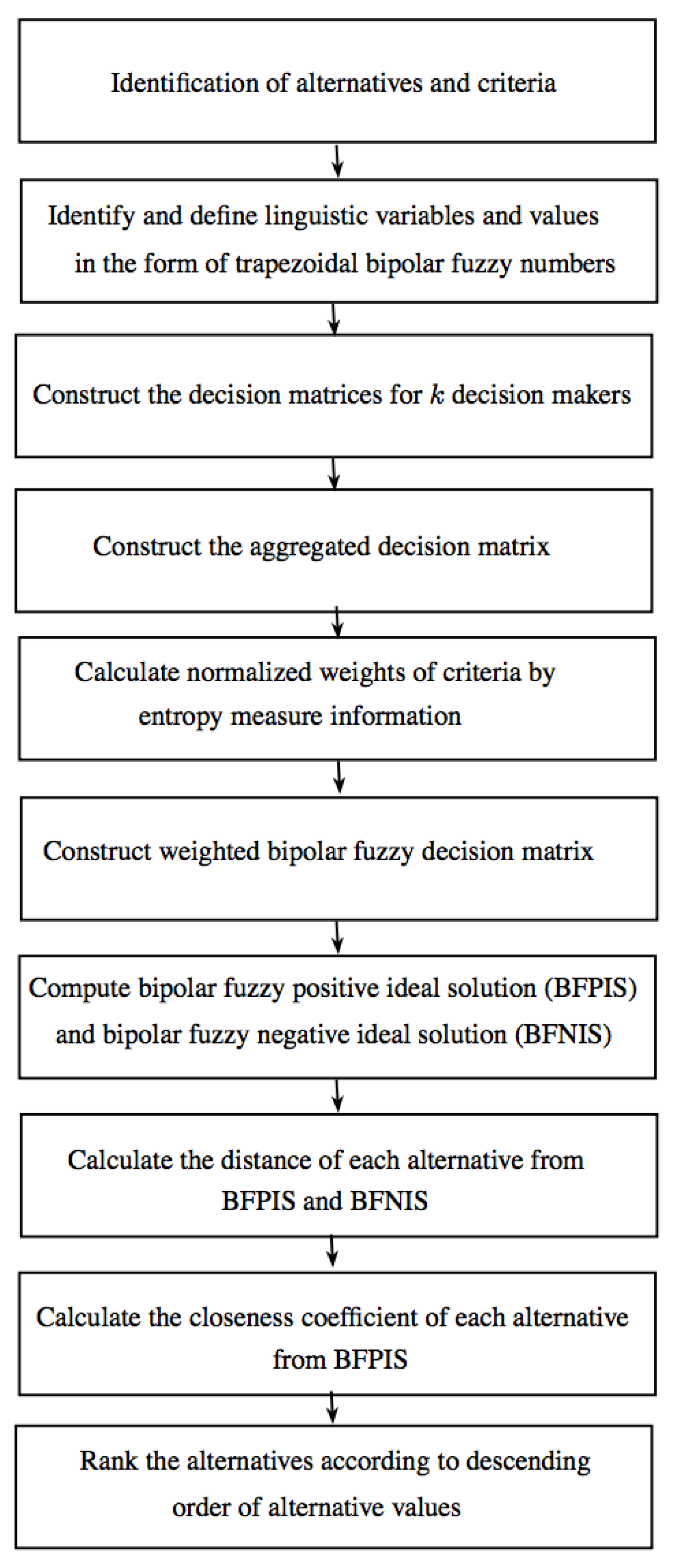
This section provides a comparative study of the proposed VIKOR method using trapezoidal bipolar fuzzy numbers with another multi-criteria decision-making method, namely, the trapezoidal bipolar fuzzy TOPSIS method, which was presented by Akram and Arshad [22]. The multi-criteria decision-making problem given in Section 4.1 is solved by the trapezoidal bipolar fuzzy TOPSIS method to make a comparison between these methods, which shows the authentication and reliability of the proposed method.

Trapezoidal Bipolar Fuzzy TOPSIS

A flow-chart of the general steps of this method is shown in Figure 6.

When solving the problem of waste treatment strategies by using trapezoidal bipolar fuzzy TOPSIS, the steps for the construction of the aggregated bipolar fuzzy decision matrix and the calculation of weights are the same as that presented in the bipolar fuzzy VIKOR method. So, we can then move to the next step and construct the weighted bipolar fuzzy decision matrix for criteria ${\mathcal{K}}_1$, ${\mathcal{K}}_2$, and ${\mathcal{K}}_3$, which is shown in

Table 24. Weighted bipolar fuzzy decision matrix.

	${\mathcal{K}}_1$	${\mathcal{K}}_2$	${\mathcal{K}}_3$
${\mathcal{T}}_1$	$\langle (0.038,0.049,0.051,0.064),$	$\langle (0.099,0.141,0.141,0.198),$	$\langle (0.163,0.233,0.233,0.326),$
	$(0.0,0.011,0.017,0.019)\rangle$	$(0.025,0.099,0.124,0.174)\rangle$	$(0.041,0.163,0.204,0.286)\rangle$
${\mathcal{T}}_2$	$\langle (0.026,0.049,0.053,0.064),$	$\langle (0.198,0.223,0.248,0.248),$	$\langle (0.163,0.233,0.233,0.326),$
	$(0.0,0.015,0.021,0.045)\rangle$	$(0.0,0.025,0.05,0.05)\rangle$	$(0.041,0.163,0.204,0.286)\rangle$
${\mathcal{T}}_3$	$\langle (0.026,0.045,0.047,0.064),$	$\langle (0.099,0.174,0.181,0.248),$	$\langle (0.163,0.314,0.339,0.408),$
	$(0.0,0.017,0.024,0.045)\rangle$	$(0.0,0.067,0.092,0.174)\rangle$	$(0.0,0.094,0.135,0.286)\rangle$
${\mathcal{T}}_4$	$\langle (0.026,0.04,0.04,0.051),$	$\langle (0.149,0.191,0.198,0.248),$	$\langle (0.245,0.339,0.367,0.408),$
	$(0.006,0.019,0.026,0.045)\rangle$	$(0.0,0.042,0.067,0.074)\rangle$	$(0.0,0.053,0.094,0.122)\rangle$
${\mathcal{T}}_5$	$\langle (0.038,0.045,0.045,0.051),$	$\langle (0.099,0.141,0.141,0.198),$	$\langle (0.163,0.233,0.233,0.326),$
	$(0.006,0.013,0.019,0.019)\rangle$	$(0.025,0.099,0.124,0.174)\rangle$	$(0.041,0.163,0.204,0.286)\rangle$

, whereas the weighted bipolar fuzzy decision matrix for criteria ${\mathcal{K}}_4$ and ${\mathcal{K}}_5$ is given in

Table 25. Weighted bipolar fuzzy decision matrix.

	${\mathcal{K}}_4$	${\mathcal{K}}_5$
${\mathcal{T}}_1$	$\langle (0.067,0.093,0.101,0.112),$	$\langle (0.017,0.089,0.096,0.134),$
	$(0.0,0.015,0.026,0.034)\rangle$	$(0.017,0.062,0.079,0.134)\rangle$
${\mathcal{T}}_2$	$\langle (0.067,0.093,0.101,0.112),$	$\langle (0.067,0.106,0.113,0.168),$
	$(0.0,0.015,0.026,0.034)\rangle$	$(0.0,0.062,0.079,0.118)\rangle$
${\mathcal{T}}_3$	$\langle (0.045,0.064,0.064,0.09),$	$\langle (0.017,0.101,0.113,0.168),$
	$(0.011,0.049,0.056,0.078)\rangle$	$(0.0,0.055,0.072,0.134)\rangle$
${\mathcal{T}}_4$	$\langle (0.067,0.093,0.101,0.112),$	$\langle (0.101,0.129,0.134,0.168),$
	$(0.0,0.015,0.026,0.034)\rangle$	$(0.0,0.029,0.045,0.05)\rangle$
${\mathcal{T}}_5$	$\langle (0.067,0.078,0.078,0.09),$	$\langle (0.067,0.106,0.106,0.134),$
	$(0.011,0.022,0.034,0.034)\rangle$	$(0.017,0.05,0.067,0.118)\rangle$

.

The bipolar fuzzy positive ideal solution (BFPIS) and bipolar fuzzy negative ideal solution (BFNIS) for each criteria ${\mathcal{K}}_{\beta }$ may be computed as:

$$\begin{array}{c}\hfill \begin{array}{cc}\hfill BFPIS=\{& \langle (0.038,0.049,0.051,0.064),(0.0,0.011,0.017,0.019)\rangle ,\hfill \\ \hfill & \langle (0.198,0.223,0.248,0.248),(0.0,0.025,0.05,0.05)\rangle ,\hfill \\ \hfill & \langle (0.163,0.233,0.233,0.326),(0.041,0.163,0.204,0.286)\rangle ,\hfill \\ \hfill & \langle (0.067,0.093,0.101,0.112),(0.0,0.015,0.026,0.034)\rangle ,\hfill \\ \hfill & \langle (0.017,0.089,0.096,0.134),(0.017,0.062,0.079,0.134)\rangle \},\hfill \end{array}\end{array}$$

$$\begin{array}{c}\hfill \begin{array}{cc}\hfill BFNIS=\{& \langle (0.026,0.04,0.04,0.051),(0.006,0.019,0.026,0.045)\rangle ,\hfill \\ \hfill & \langle (0.099,0.141,0.141,0.198),(0.025,0.099,0.124,0.174)\rangle ,\hfill \\ \hfill & \langle (0.245,0.339,0.367,0.408),(0.0,0.053,0.094,0.122)\rangle ,\hfill \\ \hfill & \langle (0.045,0.064,0.064,0.09),(0.011,0.049,0.056,0.078)\rangle ,\hfill \\ \hfill & \langle (0.101,0.129,0.134,0.168),(0.0,0.029,0.045,0.05)\rangle \}.\hfill \end{array}\end{array}$$

The distance $E_{\alpha }^{+}$ of each alternative from BFPIS and the distance $E_{\alpha }^{-}$ of each alternative from BFNIS, as well as the results of the closeness coefficients, are shown in

Table 26. Closeness coefficient to BFPIS.

Alternatives	Distance from BFPIS (${\mathit{E}}_{\mathit{\alpha }}^{+}$)	Distance from BFNIS (${\mathit{E}}_{\mathit{\beta }}^{-}$)	Closeness Coefficient
${\mathcal{T}}_1$	$0.169$	$0.250$	$0.597$
${\mathcal{T}}_2$	$0.053$	$0.291$	$0.846$
${\mathcal{T}}_3$	$0.202$	$0.178$	$0.468$
${\mathcal{T}}_4$	$0.258$	$0.133$	$0.340$
${\mathcal{T}}_5$	$0.177$	$0.234$	$0.569$

. According to these values of closeness coefficients, the alternatives are ranked in descending order, such as:

$$\begin{array}{c}\hfill {\mathcal{T}}_2\succ {\mathcal{T}}_1\succ {\mathcal{T}}_5\succ {\mathcal{T}}_3\succ {\mathcal{T}}_4.\end{array}$$

The results of these two methods applying for the selection of waste treatment strategies is given in

Table 27. Comparative study.

Methods	Final Results of Alternatives	Ranking of Alternatives
Trapezoidal bipolar fuzzy TOPSIS	$0.597$, $0.846$, $0.468$, $0.340$, $0.569$	${\mathcal{T}}_2\succ {\mathcal{T}}_1\succ {\mathcal{T}}_5\succ {\mathcal{T}}_3\succ {\mathcal{T}}_4$
Trapezoidal bipolar fuzzy VIKOR	$0.423$, $0.0$, $0.646$, $1.0$, $0.488$	${\mathcal{T}}_2\succ {\mathcal{T}}_1\succ {\mathcal{T}}_5\succ {\mathcal{T}}_3\succ {\mathcal{T}}_4$

.

6. Comparison of Trapezoidal Bipolar Fuzzy VIKOR with Fuzzy VIKOR

• Bipolar fuzzy sets improve the performance of well-established structures for decision-making, because they provide two-sided information for evaluating the alternatives with respect to each criteria. Bipolarity is essential to recognize positive data, which specifies what is ensured to be conceivable, as well as negative data, which specifies what is prohibited, or most likely false. In a different interpretation, two-sided information appears in the context of necessary and possible consequences [28]. Bipolar fuzzy numbers, as an extension of bipolar fuzzy subsets, are defined on the real line, and they can be used more appropriately for decision-making. The linguistic terms or values are induced by trapezoidal bipolar fuzzy linguistic variables, in which the interval for a positive membership degree shows the satisfaction behavior of an alternative towards a criterion. On the other hand, the interval for a negative membership degree represents the dissatisfaction of that alternative based on the criteria. We have used the trapezoidal bipolar fuzzy VIKOR approaches for evaluation, or to obtain the compromise solution. Our motivation lies in real-world problems where we find two-sided (instead of one-sided) information, as we have described in the examples.
• Crisp or fuzzy sets only provide us with one-sided information for making decisions. Put differently, we can say that we only have the information about the satisfaction degree of the alternatives under the corresponding criteria. By using these set structures, we are unable to take advantage of any information about the dissatisfaction degree of these alternatives with respect to the conflicting criteria. We have thus presented the trapezoidal bipolar fuzzy VIKOR method for a compromising solution as an improvement of previous successful versions of the VIKOR method.

7. Insights of This Method

• Our version of the VIKOR method is a generalized form of other existing VIKOR methods, as it first deals with bipolar fuzzy information or data.
• The Shannon entropy concept for weights calculation is used to avoid the personal interest or bias of the decision-makers towards the criteria.
• Linguistic variables parameterized by trapezoidal bipolar fuzzy numbers are used instead of bipolar fuzzy sets, since they provide more suitable results.
• Two different applications using this method are discussed.

8. Conclusions

The VIKOR method is an efficient and popular multi-attribute decision-making approach that combines the simplicity of the calculations and accuracy of the solutions. The goal of this method is to produce an ordering from a set of possible actions or alternatives, and to determine a compromise solution in multi-criteria decision-making problems under conflicting criteria. Decision-making is quite natural when the evaluation of the alternatives depends on only one criterion—in this situation, the category with the highest preference value is chosen. However, when the decision-makers face problems with having multiple criteria, their strategy becomes much more complicated. In the context of criteria multiplicity, decision-makers must choose a suitable MADM methodology that can take full advantage of the information at their disposal.

In this research article, we have put forward the technique and procedure of a MADM method in a bipolar fuzzy environment, and called it the trapezoidal bipolar fuzzy VIKOR method. We resorted to linguistic variables parameterized by trapezoidal bipolar fuzzy numbers for the preference ratings of alternatives with respect to conflicting criteria. A ranking function of bipolar fuzzy numbers was then applied to construct a decision matrix with real entries. The weights of the criteria were calculated by deploying the entropy concept of weight measuring. We applied the proposed method to two real-world problems, including the selection of waste treatment strategies, as well as the selection of a site for a thermal power station. Finally, we also provided a comparative analysis of the VIKOR and TOPSIS methods using trapezoidal bipolar fuzzy numbers.

Therefore, our work contributes to the expansion of the scope of application of an acclaimed methodology for decision-making.

References

- Churchman, C.W.; Ackoff, R.L. An approximate measure of value. J. Oper. Res. Soc. Am. 1954, 2, 172–187. [Google Scholar] [CrossRef]
- Saaty, T.L. Axiomatic foundation of the analytic hierarchy process. Manag. Sci. 1986, 32, 841–855. [Google Scholar] [CrossRef]
- Opricovic, S.; Tzeng, G.H. Compromise solution by MCDM methods: A comparative analysis of VIKOR and TOPSIS. Eur. J. Oper. Res. 2004, 156, 445–455. [Google Scholar] [CrossRef]
- Hwang, C.L.; Yoon, K. Multiple Attribute Decision-Making Methods and Applications; Springer: Berlin, Germany, 1981. [Google Scholar]
- Brans, J.P.; Vincke, P.; Mareschal, B. How to select and how to rank projects: The PROMETHEE method. Eur. J. Oper. Res. 1986, 24, 228–238. [Google Scholar] [CrossRef]
- Benayoun, R.; Roy, B.; Sussman, B. ELECTRE: Une Méthode pour Guider le Choix en Presence de Points de vue Multiples; Note de travail, 49; SEMA-METRA International, Direction Scientifique: Paris, France, 1966. [Google Scholar]
- Julong, D. Introduction to grey system theory. J. Grey Syst. 1989, 1, 1–24. [Google Scholar]
- Bellman, R.E.; Zadeh, L.A. Decision-making in a fuzzy environment. Manag. Sci. 1970, 4, 141–164. [Google Scholar] [CrossRef]
- Opricovic, S. A compromise solution in water resources planning. Water Resour. Manag. 2009, 23, 1549–1561. [Google Scholar] [CrossRef]
- Chang, C.L.; Hsu, C.H. Applying a modified VIKOR method to classify land subdivisions according to watershed vulnerability. Water Resour. Manag. 2011, 25, 301–309. [Google Scholar] [CrossRef]
- El-Santawy, M.F. A VIKOR method for solving personnel training selection problem. Int. J. Comput. Sci. 2012, 1, 9–12. [Google Scholar]
- Opricovic, S.; Tzeng, G.H. Extended VIKOR method in comparison with outranking methods. Eur. J. Oper. Res. 2007, 178, 514–529. [Google Scholar] [CrossRef]
- Sanayei, A.; Mousavi, S.F.; Yazdankhah, A. Group decision-making process for supplier selection with VIKOR under fuzzy environment. Expert Syst. Appl. 2010, 37, 24–30. [Google Scholar] [CrossRef]
- Shemshadi, A.; Shirazi, H.; Toreihi, M.; Tarokh, M.J. A fuzzy VIKOR method for supplier selection based on entropy measure for objective weighting. Expert Syst. Appl. 2011, 38, 12160–12167. [Google Scholar] [CrossRef]
- Lihong, M.; Yanping, Z.; Zhiwei, Z. Improved VIKOR Algorithm Based on AHP and Shannon Entropy in the Selection of Thermal Power Enterprise’s Coal Suppliers. In Proceedings of the 2008 International Conference on Information Management, Innovation Management and Industrial Engineering, Taipei, Taiwan, 19–21 December 2008; pp. 129–133. [Google Scholar]
- Wang, T.C.; Lee, H.D. Developing a fuzzy TOPSIS approach based on subjective weights and objective weights. Expert Syst. Appl. 2009, 36, 8980–8985. [Google Scholar] [CrossRef]
- Kim, Y.; Chung, E.S. Fuzzy VIKOR approach for assessing the vulnerability of the water supply to climate change and variability in South Korea. Appl. Math. Model. 2013, 37, 9419–9430. [Google Scholar] [CrossRef]
- Luo, X.; Wang, X. Extended VIKOR method for intuitionistic fuzzy multiattribute decision-making based on a new distance measure. Math. Probl. Eng. 2017, 2017, 4072486. [Google Scholar] [CrossRef]
- Zhang, W.R. Bipolar fuzzy sets and relations: A computational framework for cognitive modeling and multiagent decision analysis. In Proceedings of the IEEE Conference Fuzzy Information Processing Society Biannual Conference, San Antonio, TX, USA, 18–21 December 1994; pp. 305–309. [Google Scholar]
- Zhang, W.R. (Yin) (Yang) bipolar fuzzy sets. In Proceedings of the 1998 IEEE International Conference on Fuzzy Systems Proceedings, IEEE World Congress on Computational Intelligence (Cat. No.98CH36228), Anchorage, AK, USA, 4–9 May 1998; pp. 835–840. [Google Scholar]
- Zadeh, L.A. Fuzzy sets. Inf. Control. 1965, 8, 338–353. [Google Scholar] [CrossRef] [Green Version]
- Akram, M.; Arshad, M. A novel trapezoidal bipolar fuzzy TOPSIS method for group decision-making. Group Decis. Negot. 2019, 28, 565–584. [Google Scholar] [CrossRef]
- Alghamdi, M.A.; Alshehri, N.O.; Akram, M. Multi-criteria decision-making methods in bipolar fuzzy environment. Int. J. Fuzzy Syst. 2018, 20, 2057–2064. [Google Scholar] [CrossRef]
- Akram, M.; Shumaiza; Arshad, M. Bipolar fuzzy TOPSIS and bipolar fuzzy ELECTRE-I methods to diagnosis. Comput. Appl. Math. 2019. [Google Scholar] [CrossRef]
- Samanta, S.; Sarkar, B. A study on generalized fuzzy graphs. J. Intell. Fuzzy Syst. 2018, 35, 3405–3412. [Google Scholar] [CrossRef]
- Sarkar, B.; Samanta, S. Generalized fuzzy trees. Int. J. Comput. Intell. Syst. 2017, 10, 711–720. [Google Scholar] [CrossRef] [Green Version]
- Alcantud, J.C.R.; Biondo, A.; Giarlotta, A. Fuzzy politics I: The genesis of parties. Fuzzy Sets Syst. 2018, 349, 71–98. [Google Scholar] [CrossRef]
- Alcantud, J.C.R.; Giarlotta, A. Necessary and possible Hesitant fuzzy sets: A novel model for group decision-making. Inf. Fusion 2019, 46, 63–76. [Google Scholar] [CrossRef]
Figure 1.
Ideal and compromise solutions.
Figure 2.
Linguistic variables for cost criteria.
Figure 3.
Linguistic variables for benefit criteria.
Figure 4.
The framework for selecting the waste treatment strategy.
Figure 5.
The framework for site-selection for a thermal power station.
Figure 6.
The flow-chart of the trapezoidal bipolar fuzzy TOPSIS method.