
Logical and Geometrical Distance in Polyhedral Aristotelian Diagrams in Knowledge Representation

1
Center for Logic and Analytic Philosophy, KU Leuven, 3000 Leuven, Belgium
2
Research Group on Formal and Computational Linguistics, KU Leuven, 3000 Leuven, Belgium
*
Author to whom correspondence should be addressed.
Symmetry 2017, 9(10), 204; https://doi.org/10.3390/sym9100204
Submission received: 28 August 2017
/
Revised: 14 September 2017
/
Accepted: 27 September 2017
/
Published: 29 September 2017
Abstract
:Aristotelian diagrams visualize the logical relations among a finite set of objects. These diagrams originated in philosophy, but recently, they have also been used extensively in artificial intelligence, in order to study (connections between) various knowledge representation formalisms. In this paper, we develop the idea that Aristotelian diagrams can be fruitfully studied as geometrical entities. In particular, we focus on four polyhedral Aristotelian diagrams for the Boolean algebra , viz. the rhombic dodecahedron, the tetrakis hexahedron, the tetraicosahedron and the nested tetrahedron. After an in-depth investigation of the geometrical properties and interrelationships of these polyhedral diagrams, we analyze the correlation (or lack thereof) between logical (Hamming) and geometrical (Euclidean) distance in each of these diagrams. The outcome of this analysis is that the Aristotelian rhombic dodecahedron and tetrakis hexahedron exhibit the strongest degree of correlation between logical and geometrical distance; the tetraicosahedron performs worse; and the nested tetrahedron has the lowest degree of correlation. Finally, these results are used to shed new light on the relative strengths and weaknesses of these polyhedral Aristotelian diagrams, by appealing to the congruence principle from cognitive research on diagram design.
1. Introduction
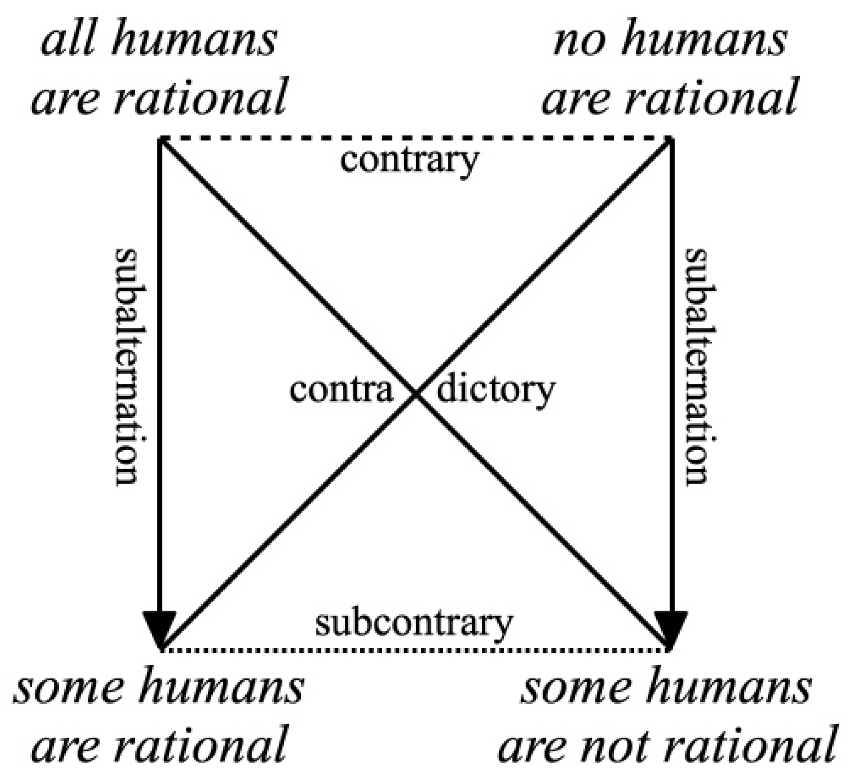
Aristotelian diagrams visualize the logical relations among a finite set of elements from some logical, lexical or conceptual system. The historical origins of these diagrams can ultimately be traced back to the logical works of Aristotle and his commentators [1]. The oldest and most widely-known example is the so-called ‘square of opposition’ for the categorical statements from Aristotle’s logical system of syllogistics; cf. Figure 1. Throughout history, distinguished philosophers such as John Buridan, Gottfried Leibniz and Gottlob Frege have made use of squares, but also larger, more complex Aristotelian diagrams to illustrate and explain their theorizing [2,3,4]. However, because of the ubiquity of the logical relations that they visualize, Aristotelian diagrams are now also used in other scientific and engineering disciplines, such as cognitive science [5,6], neuroscience [7], natural language processing [8], law [9,10,11], linguistics [12,13,14,15] and artificial intelligence. Within the latter field, Aristotelian diagrams have been used to study various logic-based approaches to knowledge representation, including fuzzy logic [16,17,18,19,20], modal-epistemic logic [21,22,23,24,25] and probabilistic logic [26,27,28]. Furthermore, Aristotelian diagrams are also used extensively to study (the connections between) other types of knowledge representation formalisms, such as formal argumentation theory [29,30,31,32], fuzzy set theory [33,34,35,36], formal concept analysis and possibility theory [37,38,39], rough set theory [37,40,41], multiple-criteria decision-making [42,43,44] and the theory of logical and analogical proportions [45,46,47,48,49]. In sum, then, Aristotelian diagrams have come to serve as visual tools that greatly facilitate communication, research and teaching in a wide variety of disciplines that deal with logical reasoning in all its facets.
In the research program of logical geometry (see www.logicalgeometry.org), we study Aristotelian diagrams as objects of independent mathematical interest, i.e., regardless of any of their specific applications. We focus on logical issues such as informativity, Boolean complexity and logic-sensitivity [50,51,52], but also on more visual/diagrammatic aspects, such as informational vs. computational equivalence of Aristotelian diagrams [53,54,55]. One of the crucial insights in this area is that Aristotelian diagrams can also be fruitfully seen as truly geometrical entities and studied by means of tools and techniques such as projection matrices, Euclidean distance, symmetry groups, etc. [54,55,56,57]. (This hybrid perspective on diagrams, treating them simultaneously as diagrammatic visualizations of an underlying abstract structure and as geometrical entities by themselves, can also be found in crystallography [58,59].) The importance of this geometrical approach is further highlighted by the following observation: although most Aristotelian diagrams that have been used in the literature so far are based on fairly simple, two-dimensional polygons such as squares (cf. Figure 1) and regular hexagons and octagons, in recent years, various researchers have also started using more visually complex, three-dimensional Aristotelian diagrams, based on polyhedra such as cubes, cuboctahedra and rhombic dodecahedra [38,60,61].
The present paper further develops and refines this geometrical perspective on Aristotelian diagrams. In particular, we will consider four three-dimensional, polyhedral Aristotelian diagrams that have recently been used to visualize the Boolean algebra , viz. the rhombic dodecahedron, the tetrakis hexahedron, the tetraicosahedron, and the nested tetrahedron. (In his research on paraconsistent logic, Béziau [62] has used various other Aristotelian diagrams, such as hexagons and octagons, but also another polyhedron, viz. a stellar rhombic dodecahedron. The precise logical and geometrical relationship between Béziau’s polyhedral Aristotelian diagram and the ones discussed in this paper is discussed in more detail in [63].) This case study is especially relevant in the context of artificial intelligence, since each of these four visualizations has recently been used in AI-related research. In particular, the rhombic dodecahedron has been used in research on modal logic and dynamic epistemic logic [22,61], the tetrakis hexahedron and tetraicosahedron have been used to investigate modal logic [25,60,64,65], and the nested tetrahedron has been used to study (connections between) the knowledge representation formalisms of rough set theory, formal concept analysis and possibility theory [38,40]. (However, it should also be noted that our focus on precludes us from studying Aristotelian diagrams for knowledge representation formalisms that go beyond a Boolean setup, such as fuzzy logic and set theory [16,17,18,19,20,33,34,35,36]. The systematic (logical and diagrammatic) investigation of such non-classical Aristotelian diagrams is a matter of ongoing research.)
The paper makes two crucial new contributions to this line of research. First of all, it offers a detailed investigation of the geometrical properties of, and interrelationships between, these four polyhedral Aristotelian diagrams. Some of these geometrical properties/interrelationships are immediately clear from the visual features of the polyhedra, but some of them are more abstract in nature (e.g., in the case of two polyhedra that, despite their clear visual differences, can be obtained by means of two different types of projections of one and the same higher-dimensional polytope). Secondly, it analyzes the correspondence (or lack thereof) between the logical and geometrical notions of distance in each of these four polyhedral Aristotelian diagrams. Logical distance is defined in terms of the Hamming distance between the bitstring representations of the elements of , whereas geometrical distance is identified with the Euclidean distance between each polyhedron’s vertices corresponding to those bitstring representations. The results of this comparative analysis will then be used to shed new light on the relative strengths and weaknesses of these polyhedral Aristotelian diagrams, by appealing to the congruence principle from diagram design [66,67].
As will be indicated throughout the remainder of the paper, there exists some earlier work on polyhedral Aristotelian diagrams for . For example, Moretti [68] sketches the outlines of a comparison between the Aristotelian tetraicosahedron and nested tetrahedron, but it goes into far less geometrical detail than the present paper, and does not deal with the Aristotelian rhombic dodecahedron and tetrakis hexahedron. Similarly, Smessaert et al. [63,69] compare the Aristotelian rhombic dodecahedron, tetrakis hexahedron and tetraicosahedron, but these studies again go into far less geometrical detail than the present paper and do not address the Aristotelian nested tetrahedron. Finally, Smessaert et al. [55,57] offer an in-depth geometrical comparison of the Aristotelian rhombic dodecahedron and nested tetrahedron for , but these papers do not deal with the Aristotelian tetrakis hexahedron and tetraicosahedron.
The paper is organized as follows. Section 2 briefly presents the Boolean algebra , its bitstring representation and its polyhedral Hasse diagram. Section 3, then provides a detailed overview of the four polyhedral Aristotelian diagrams for that have been proposed in the literature, focusing on their geometrical properties and interrelations, as well as on their logical applications. Section 4 introduces the notions of logical (Hamming) distance and geometrical (Euclidean) distance and analyzes how closely these two notions of distance are correlated in each of the four polyhedral Aristotelian diagrams for . Furthermore, the results of this comparative analysis are interpreted in light of the congruence principle from cognitive studies on diagram design. Finally, Section 5 briefly summarizes the results obtained in this paper and offers some questions for further research.
2. The Boolean Algebra and Its Polyhedral Hasse Diagram
The notion of a Boolean algebra is well-known in abstract algebra [70]. As a special case of the Stone representation theorem, every finite Boolean algebra is isomorphic to the powerset of some finite set. In particular, the Boolean algebra is isomorphic to , and elements of can be represented as subsets of (the identity of the elements is irrelevant here). However, in logical geometry it is more customary to represent finite Boolean algebras by means of bitstrings [71]. In particular, the Boolean algebra is represented by means of bitstrings of length 4, i.e., (obviously, every bitstring of length 4 uniquely corresponds to (the characteristic function of) a subset of ; for example, the bitstring 1010 corresponds to the subset .) These bitstrings can be used to provide a coarse-grained semantics for fragments of a wide variety of logical systems; see [51] for the mathematical details of this technique.
In a Boolean algebra , the notion of level is inductively defined as follows: and . In the bitstring representation of , the level of a bitstring simply corresponds to its number of 1-bits; for example and . The Aristotelian relations are usually defined for formulas of some given logical system [50], but this can easily be generalized to arbitrary Boolean algebras [72,73]. In the specific case of the bitstring representation of , we say that two bitstrings are:
| contradictory () | iff | and | , | |
| contrary (C) | iff | and | , | |
| subcontrary () | iff | and | , | |
| in subalternation () | iff | and | . |
In the definition of , the condition that captures the informal idea that contradictories ‘cannot be true together’, while the condition that captures the informal idea that they ‘cannot be false together’ [72,73]. In the definitions of and , one of the two identity conditions of is negated: contraries can be false together, while subcontraries can be true together. The set of Aristotelian relations is fundamentally hybrid in nature: the opposition relations , and are defined using the top and bottom elements of , while the implication relation is defined in terms of the bitstrings and themselves [50].
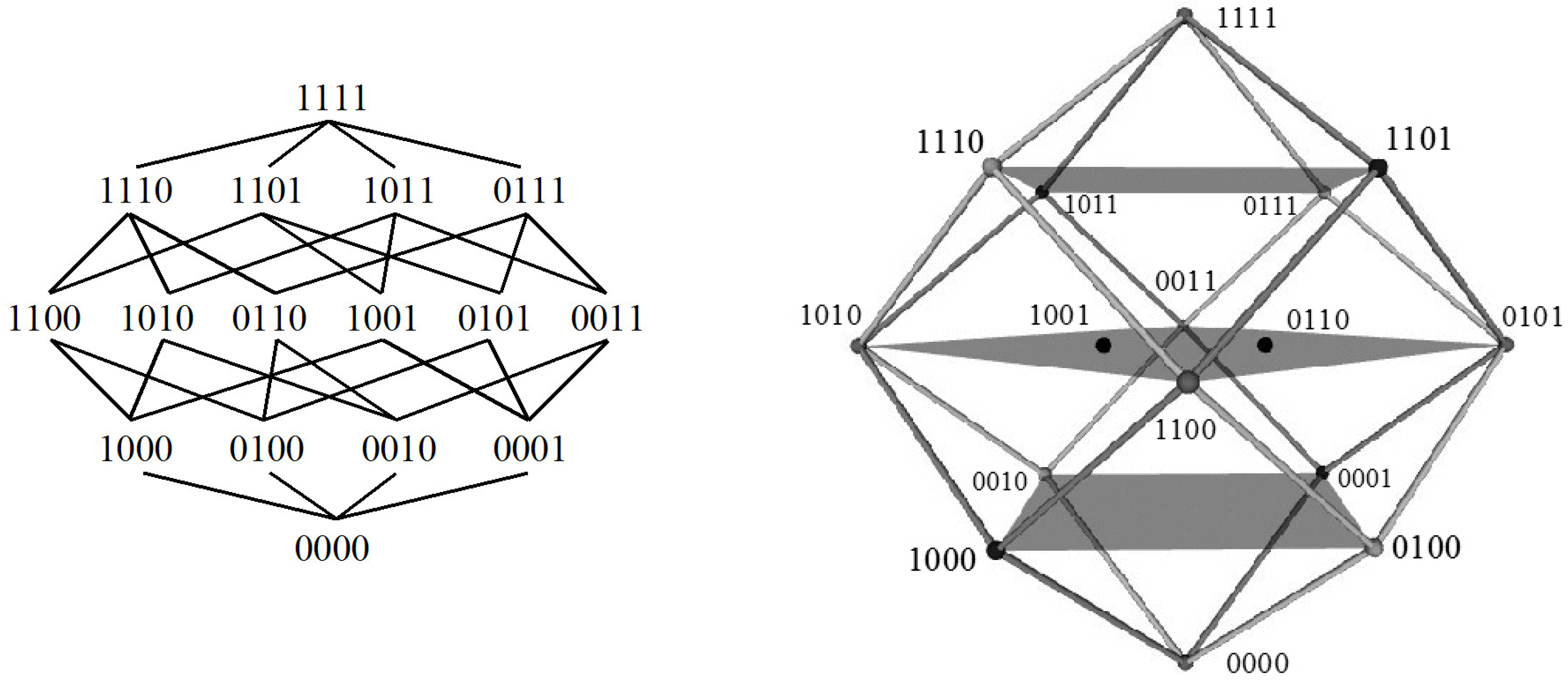
Since Boolean algebras are a particular kind of partially ordered sets, they can be visualized by means of Hasse diagrams [74]. The standard, two-dimensional Hasse diagram for (the bitstring representation of) is shown in Figure 2a. This diagram visualizes negation by means of central symmetry: contradictory bitstrings are located at diametrically opposed vertices of the diagram. Furthermore, in this Hasse diagram, the logical ordering of levels corresponds to the vertical geometrical ordering of lines, from at the bottom of the diagram up to at the top. However, several authors have also made use of polyhedra to provide alternative, three-dimensional Hasse diagrams for [75,76]. In particular, Figure 2b shows a Hasse diagram for based on a rhombic dodecahedron. Just like its two-dimensional counterpart, this polyhedral Hasse diagram also visualizes negation by means of central symmetry, whereas the logical ordering of levels now corresponds to the vertical geometrical ordering of planes, from at the bottom of the diagram up to at the top.
The geometrical properties of the rhombic dodecahedron will be discussed in more detail in the next section. (This geometrical information will play an important role in our discussion of the (dis)similarities between the rhombic dodecahedron and the other polyhedra that are introduced in Section 3, and is thus most naturally at home in that section.) For now, it suffices to emphasize that the rhombic dodecahedron is a very natural choice for a polyhedral Hasse diagram for , because of a specific combination of logical and geometrical considerations. On the one hand, the (bitstring representation of the) Boolean algebra can always be represented by means of an n-dimensional hypercube, with the logical bit values 1/0 corresponding to the Euclidean coordinates [77] (for example, the bitstring 10101 in corresponds to the vertex in ). In particular, the Boolean algebra can thus be represented by means of a four-dimensional hypercube, i.e., a tesseract. On the other hand, it is well-known that the vertex-first parallel projection of a tesseract from four-space into three-space is exactly a rhombic dodecahedron [56]. In particular, the rhombic dodecahedron in Figure 2b can be seen as the vertex-first parallel projection of a tesseract along the projection axis defined by (the vertices corresponding to) the bitstrings 1001 and 0110, because those are precisely the two bitstrings that end up in the center of polyhedron, rather than on its exterior surface. Actually, in order to avoid that 1001 and 0110 entirely coincide with each other in the center of the polyhedron, a slight distortion in the projection axis has been introduced; this procedure is standard [78], and the Hasse rhombic dodecahedron can therefore be said to be a ‘quasi-vertex-first projection’ of a tesseract [56].
3. Polyhedral Aristotelian Diagrams for
In the previous section, we have introduced the Boolean algebra and a specific polyhedral Hasse diagram for it. In the remainder of this paper, however, we will rather focus on polyhedral Aristotelian diagrams for . The latter emphasize different logical aspects of ; in particular, they focus on clearly visualizing the Aristotelian relations holding among the elements of . In order to achieve this goal, other logical information is distorted or left out altogether; for example, the top and bottom elements of , i.e., the non-contingent bitstrings 1111 and 0000, are not shown at all in an Aristotelian diagram (because they enter into abundantly many ‘vacuous’ Aristotelian relations [50]), and the logical ordering of levels is no longer reflected in a vertical ordering of planes.
At least four different polyhedral Aristotelian diagrams for have been proposed in the literature. These diagrams all represent the same logical structure (viz. ), but they achieve this by means of very different visual means. In Larkin and Simon’s terminology [79], these Aristotelian diagrams are informationally equivalent, but they need not be computationally equivalent, in the sense that the visual differences between them may significantly influence user comprehension. In this section, we will provide an in-depth comparative overview of these four polyhedral Aristotelian diagrams for .
3.1. The Aristotelian Rhombic Dodecahedron for
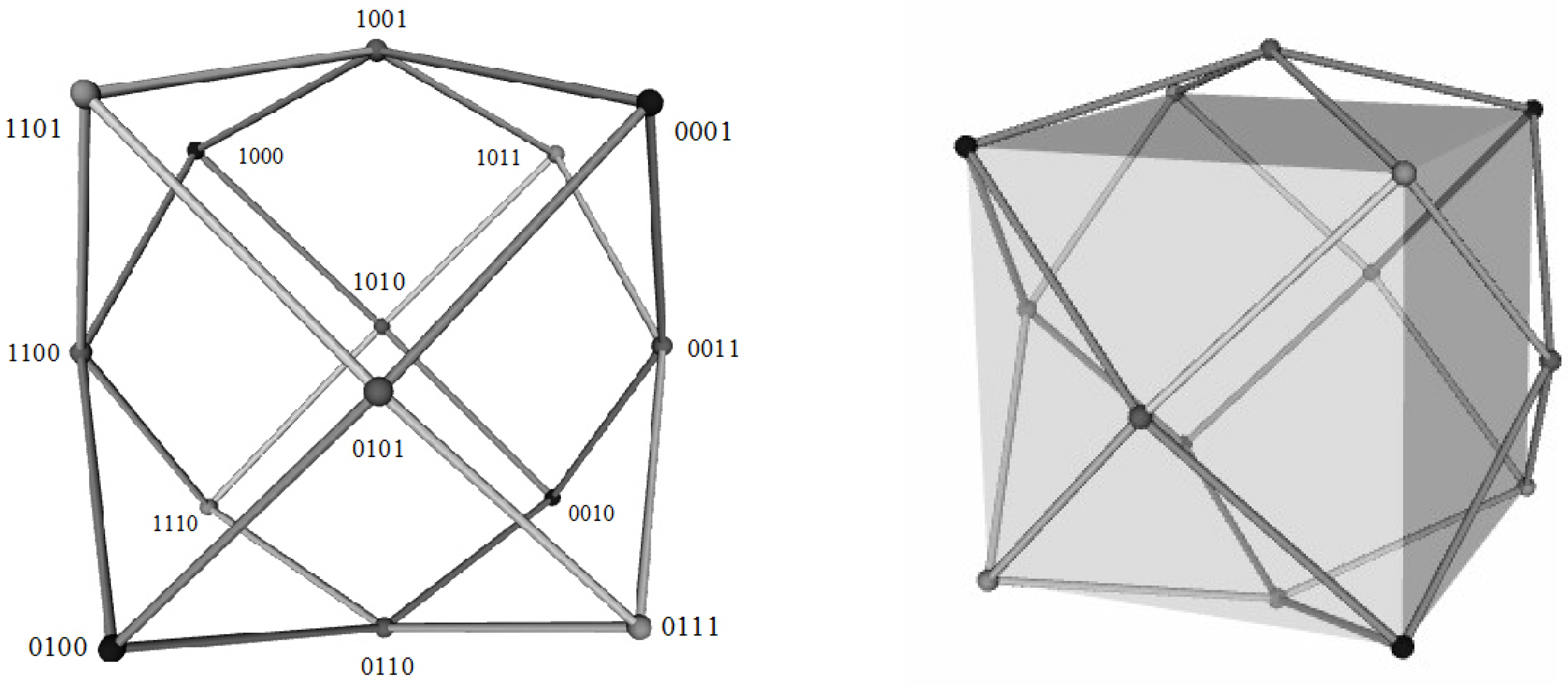
We start our overview by considering the Aristotelian rhombic dodecahedron (RDH) for , as shown in Figure 3a. This Aristotelian diagram was first proposed by Smessaert [61] in the context of his research on generalized quantifiers and modal logic and later adopted by Demey [22] in his work on public announcement logic. The Hasse diagram discussed in Section 2 and the Aristotelian diagram considered here are both based on a rhombic dodecahedron; the only difference between these diagrams concerns how the bitstrings of are mapped onto the vertices of these rhombic dodecahedra; compare Figure 2b and Figure 3a.
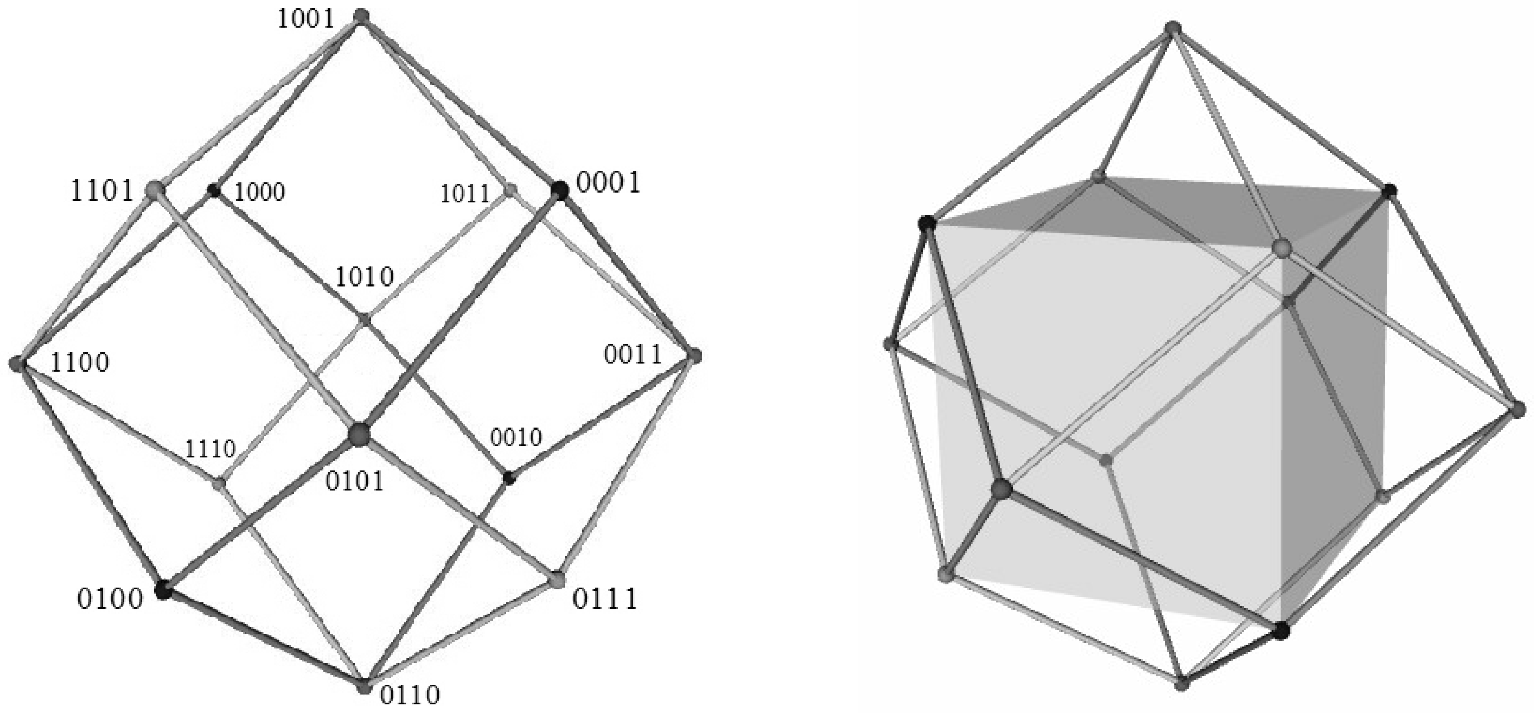
The rhombic dodecahedron has 14 vertices, 24 edges and 12 (rhombic) faces; being a convex polyhedron, it has Euler characteristic , i.e., . Note that the number of vertices () corresponds exactly to the number of contingent bitstrings of : this Boolean algebra has bitstrings in total, so after discarding 1111 and 0000, we are left with 14 contingent bitstrings. The rhombic dodecahedron is a Catalan solid [80], and has as its symmetry group the octahedral group (of order 48), which it shares with its dual polyhedron, the cuboctahedron [63,81,82]. The latter is itself an Archimedean solid and has also been used as a polyhedral Aristotelian diagram [60]. Furthermore, the rhombic dodecahedron is closely related to both the cube and the octahedron (which are themselves dual to each other), as shown in Figure 4 [63,69,83].
Just like the Hasse rhombic dodecahedron for discussed in the previous section, the Aristotelian rhombic dodecahedron for is also the vertex-first parallel projection of a tesseract, but now along the projection axis defined by (the vertices corresponding to) the bitstrings 1111 and 0000. Furthermore, since the non-contingent bitstrings 1111 and 0000 are irrelevant in Aristotelian diagrams, it is unproblematic that they exactly coincide with each other in the center of the polyhedron, and hence, there is no need to invoke a quasi-vertex-first projection. By viewing the Hasse and Aristotelian rhombic dodecahedra as two vertex-first parallel projections of a tesseract, albeit along different projection axes, we also obtain a unified geometrical explanation of their fundamental diagrammatic differences [56]. In particular, in the tesseract, the logical levels are ordered by means of hyperplanes going from (the vertex corresponding to) 0000 to (the vertex corresponding to) 1111; however, if the projection is precisely along the 1111/0000 axis, then this ordering is completely annihilated, so that the resulting Aristotelian rhombic dodecahedron no longer visually represents this ordering of levels: the -, - and -bitstrings are scattered throughout the polyhedron [55,57].
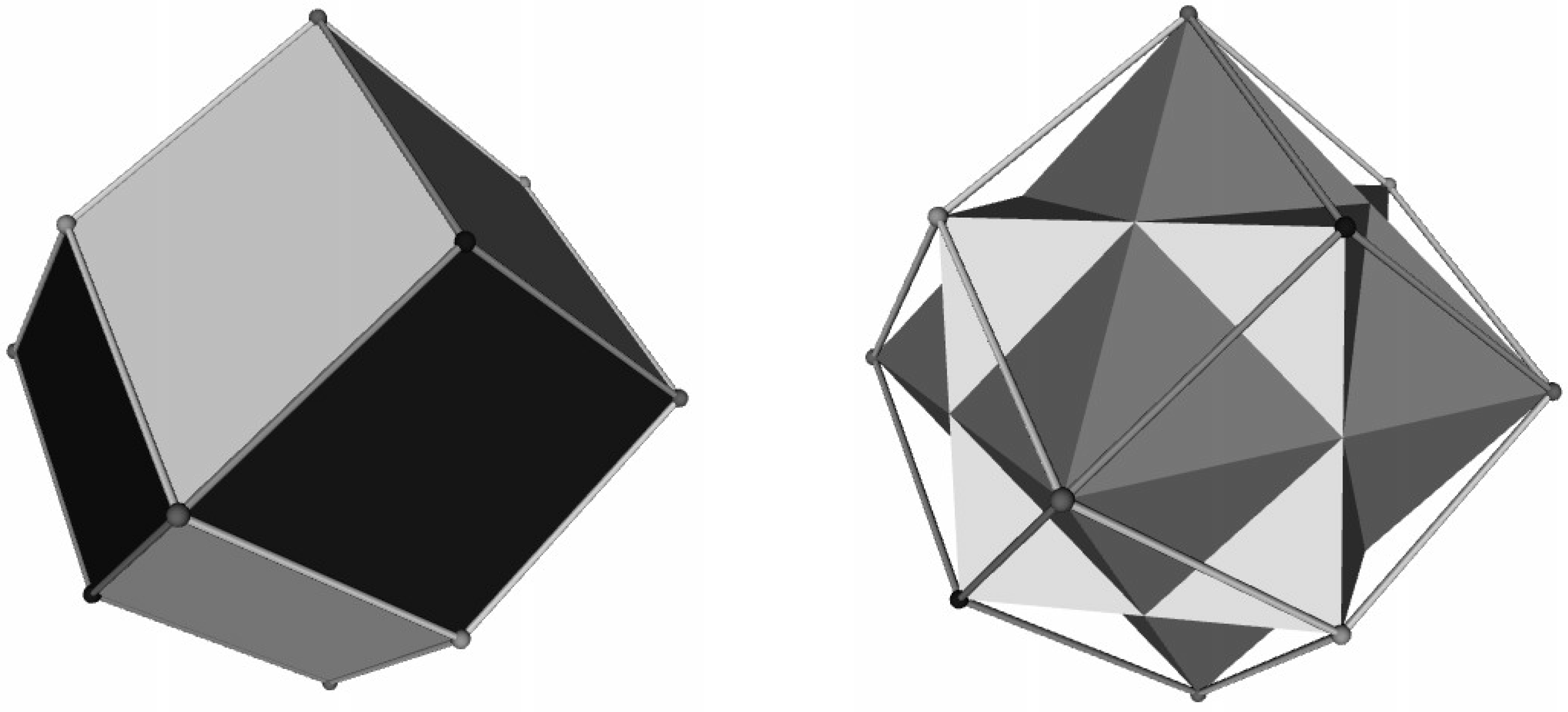
As is illustrated in Figure 3b, the rhombic dodecahedron can be seen as the result of putting a square pyramid onto each of the faces of a cube [84]. The height of these six pyramids should be such that the lateral, triangular faces of adjacent pyramids lie in the same plane and together form a single, rhombic face of the rhombic dodecahedron. It is easy to show that if the cube has edge length ℓ, this can be achieved by using pyramids of height . In these pyramids, the base is a square of edge length ℓ (viz. one of the faces of the cube), and the lateral faces are isosceles triangles (with one edge of length ℓ and two of length ); the lateral faces are at an angle of to the base. This perspective on the rhombic dodecahedron will be useful later on, when we are comparing it with other polyhedra.
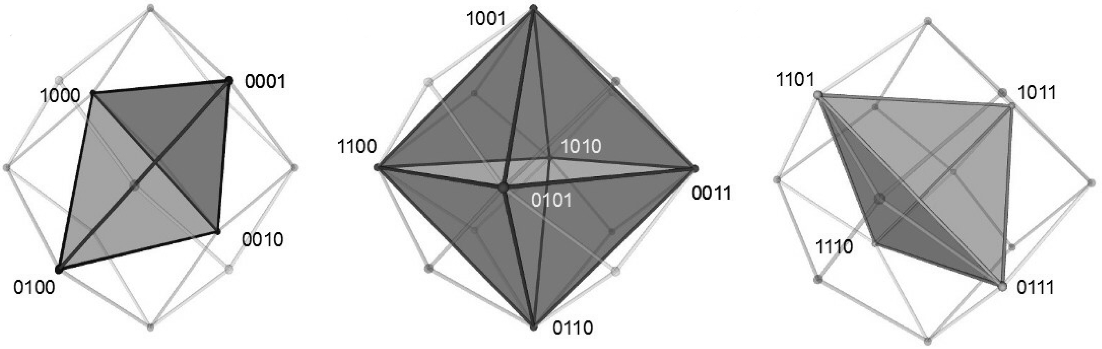
It will be convenient to fix a set of standard coordinates for the vertices of the Aristotelian rhombic dodecahedron. The coordinate function shown in Table 1 at the end of this section maps the bitstrings of onto the vertices of the Aristotelian rhombic dodecahedron [55,57]. Note that and for all bitstrings b, i.e., the top and bottom elements of coincide with each other in the center of the Aristotelian rhombic dodecahedron, and logical negation is visualized by means of central symmetry. The - and -bitstrings are mapped onto the vertices and constitute two equal-sized tetrahedra that ‘interlock’ with each other to yield a cube, whereas the -bitstrings are mapped onto the vertices , and , which constitute an octahedron; cf. Figure 5. (Of course, the vertices , and can also be seen as the tops of the pyramids that have been put on each of the cube’s six faces; cf. Figure 3b.) Note that the cube has edge length two, and hence the pyramids that are put on top of the cube’s faces have height one; for example, the top face of the cube lies in the plane ; the apex of the pyramid that is put on top of this face, lies at .
3.2. The Aristotelian Tetrakis Hexahedron for
We now turn to the Aristotelian tetrakis hexahedron (THH) (or simply: tetrahexahedron) for , which is shown in Figure 6a. This diagram was first used by Sauriol [85] in his research on the logical geometry of the propositional connectives and was later also adopted by Luzeaux et al. [25] and Pellissier [64] in their research on modal logic. (Although these latter authors [25,64] erroneously call their diagram a ‘tetraicosahedron’; cf. infra.) The tetrakis hexahedron has 14 vertices, 36 edges and 24 faces; being a convex polyhedron, it satisfies the Euler formula . Note that the number of vertices () again corresponds exactly to the number of contingent bitstrings of (cf. supra). The tetrakis hexahedron is again a Catalan solid; it is dual to the truncated octahedron, which is itself again an Archimedean solid; the symmetry group of both these polyhedra is again the octahedral group [80,81,82].
Just like the rhombic dodecahedron, the tetrakis hexahedron can be seen as the result of putting a square pyramid onto each of the faces of a cube; cf. Figure 6b (this was also noted by Sauriol [85], pp. 384–385). If the cube has edge length ℓ, the pyramids have height . In these pyramids, the base is a square of edge length ℓ (viz. one of the faces of the cube), and the lateral faces are isosceles triangles (with one edge of length ℓ and two of length ). Comparing the rhombic dodecahedron in Figure 3a and the tetrakis hexahedron in Figure 6a, we find that these two Aristotelian diagrams are very similar to each other. The crucial difference concerns the height of the six pyramids, which is much smaller in the latter than in the former ( in the pyramids of the tetrakis hexahedron versus in those of the rhombic dodecahedron). Consequently, in the tetrakis hexahedron, the pyramids’ lateral faces are at an angle of strictly less than to the base, and hence the lateral faces of adjacent pyramids no longer lie in the same plane, and thus no longer form a single, rhombic face. Taking the rhombic dodecahedron as our starting point, each of the 12 rhombic faces is thus broken into two triangular faces, which explains why the tetrakis hexahedron has twice as many faces as the rhombic dodecahedron (24 versus 12) and has 12 additional edges (36 versus 24).
We again fix a set of standard coordinates for the vertices of the Aristotelian tetrakis hexahedron. The coordinate function shown in Table 1 at the end of this section maps the bitstrings of onto the vertices of the Aristotelian tetrakis hexahedron. This coordinate function reveals the strong similarities between the Aristotelian rhombic dodecahedron and tetrakis hexahedron. First of all, note that we again have and for all bitstrings b, i.e., the top and bottom elements of coincide with each other in the center of the Aristotelian tetrakis hexahedron, and logical negation is visualized by means of central symmetry. Furthermore, the - and -bitstrings are once again mapped onto the vertices of the cube. The only difference between and concerns the coordinates for the -bitstrings, i.e., the height of the six pyramids that are put on top of the cube’s faces. Since the cube has edge length two, the pyramids that yield the tetrakis hexahedron have height ; for example, the top face of the cube lies in the plane ; the apex of the pyramid that is put on top of this face, lies at . In general, it holds that for all , which reflects the fact that in the tetrakis hexahedron, the pyramids’ apices are closer to the cube’s faces than was the case in the rhombic dodecahedron.
3.3. The Aristotelian Tetraicosahedron for
The next polyhedron to be considered, is the Aristotelian tetraicosahedron (TIH) for , which is shown in Figure 7a, and which was first used by Moretti [60,65] in his research on n-opposition theory and modal logic. (As far as we know, this polyhedron is not systematically studied in the geometrical literature on polyhedra; the term ‘tetraicosahedron’ only seems to occur in the logic-oriented research of Moretti, Pellissier and Luzeaux et al. Furthermore, this term has not been used entirely consistently in the literature; for example, Pellissier [64] and Luzeaux et al. [25] draw a tetrakis hexahedron, but call it a ‘tetraicosahedron’, while Moretti [68], conversely, draws a tetraicosahedron, but calls it a ‘tetrahexahedron’.) Just like the tetrakis hexahedron, the tetraicosahedron has 14 vertices, 36 edges and 24 faces; even though this polyhedron is not convex, it thus still satisfies the Euler formula . The tetraicosahedron does not belong to any of the well-studied families of polyhedra (cf. supra). It is easy to see, however, that its symmetry group is, once again, the octahedral group . Furthermore, the number of vertices () again corresponds exactly to the number of contingent bitstrings of (cf. supra).
Once again, the tetraicosahedron can be seen as the result of putting a square pyramid onto each of the faces of a cube; cf. Figure 7b. However, the idea is now that the lateral faces of these pyramids should be equilateral (rather than merely isosceles) triangles. It is easy to show that if the cube has edge length ℓ, this can be achieved by using pyramids of height . In such pyramids, the base is a square of edge length ℓ, and the lateral faces are equilateral triangles of edge length ℓ; these pyramids are Johnson solids [86]. Comparing the rhombic dodecahedron in Figure 3a and the tetraicosahedron in Figure 7a, we find that these two Aristotelian diagrams are, once again, very similar to each other. The crucial difference concerns the height of the six pyramids, which is much greater in the latter than in the former ( in the pyramids of the tetraicosahedron versus in those of the rhombic dodecahedron). Consequently, in the tetraicosahedron, the pyramids’ lateral faces are at an angle of strictly more than to the base, and hence the lateral faces of adjacent pyramids no longer lie in the same plane, and thus no longer form a single, rhombic face. Taking the rhombic dodecahedron as our starting point, each of the 12 rhombic faces is thus broken into two triangular faces, which explains why the tetraicosahedron has twice as many faces as the rhombic dodecahedron (24 versus 12), and has 12 additional edges (36 versus 24). Finally, another consequence of the pyramids’ greater heights is that the tetraicosahedron is not convex; for example, the bitstrings 1100 and 1001 are on two vertices of the tetraicosahedron, but the line segment between these two vertices clearly lies entirely outside this polyhedron; cf. Figure 7a.
It will again be convenient to fix a set of standard coordinates for the vertices of the Aristotelian tetraicosahedron. The coordinate function shown in Table 1 at the end of this section maps the bitstrings of onto the vertices of the Aristotelian tetraicosahedron. This coordinate function reveals the strong similarities between the Aristotelian rhombic dodecahedron and tetraicosahedron. First of all, note that we again have and for all bitstrings b, i.e., the top and bottom elements of coincide with each other in the center of the Aristotelian tetraicosahedron, and logical negation is visualized by means of central symmetry. Furthermore, the - and -bitstrings are once again mapped onto the vertices of the cube. The only difference between and concerns the coordinates for the -bitstrings, i.e., the height of the six pyramids that are put on top of the cube’s faces. Since the cube has edge length two, the pyramids that yield the tetraicosahedron have height ; for example, the top face of the cube lies in the plane ; the apex of the pyramid that is put on top of this face, lies at . In general, it holds that for all , which reflects the fact that in the tetraicosahedron, the pyramids’ apices are farther removed from the cube’s faces than was the case in the rhombic dodecahedron.
3.4. The Aristotelian Nested Tetrahedron for
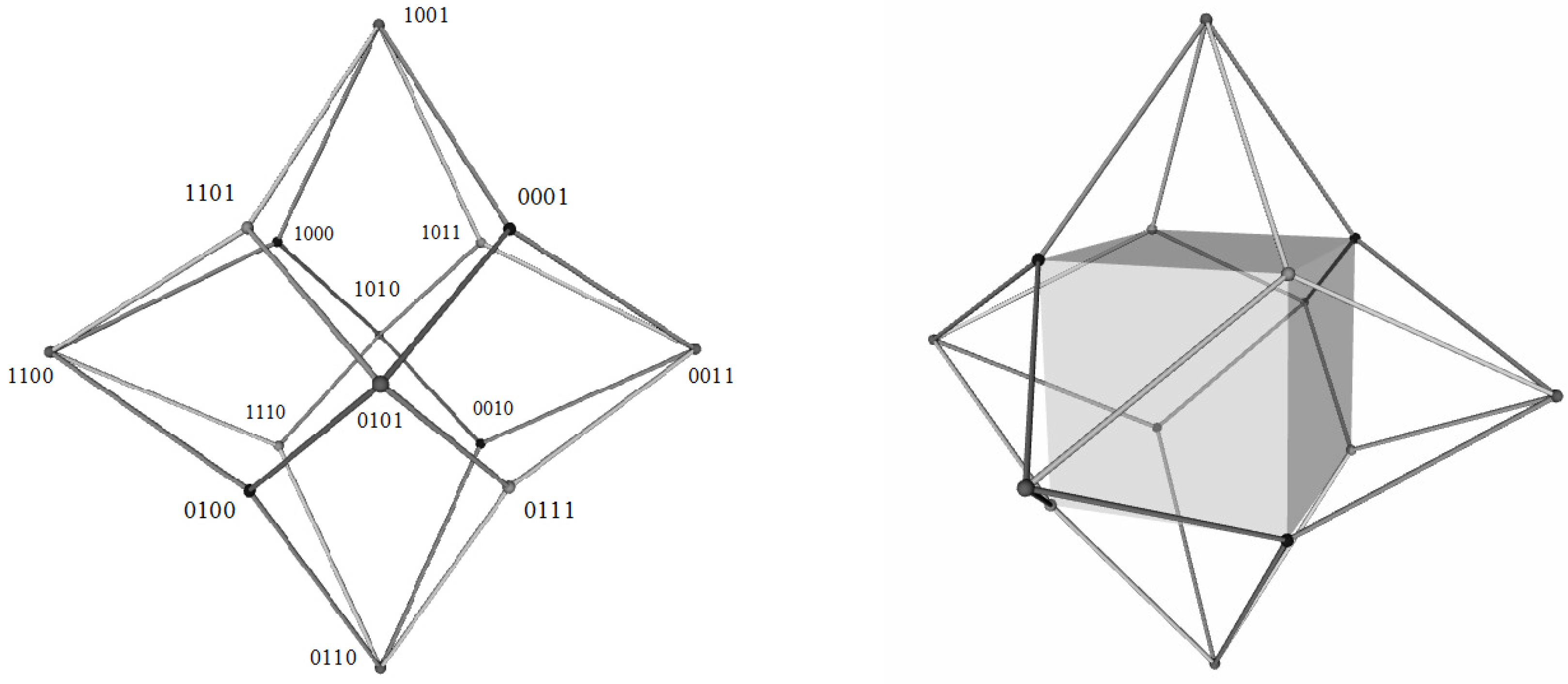
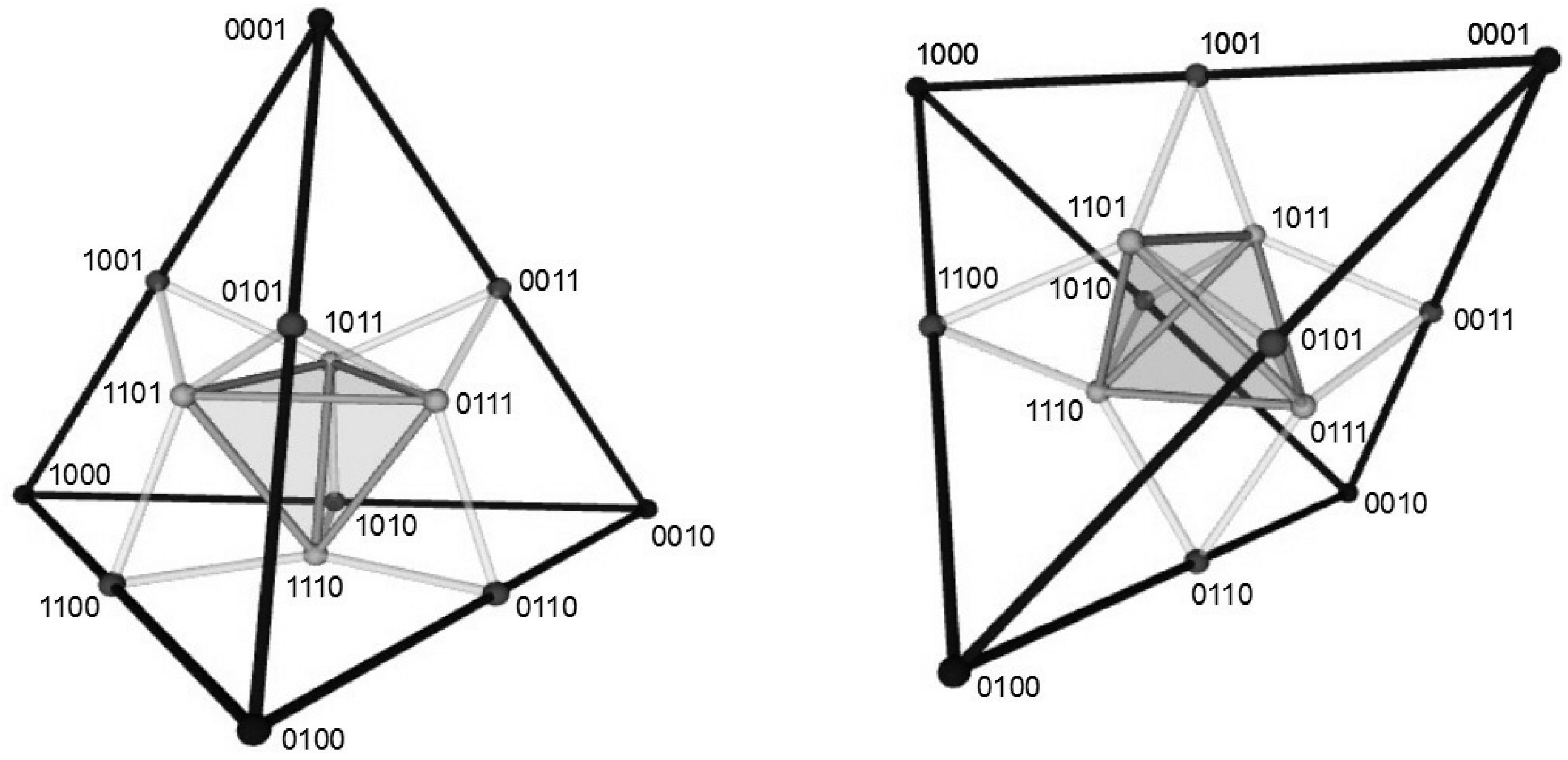
The final polyhedron to be considered, is the Aristotelian nested tetrahedron (NTH) for , as shown in Figure 8. Ciucci, Dubois and Prade have recently made use of this Aristotelian diagram in their comparative research on the logical geometry of rough set theory, formal concept analysis and possibility theory [38,40]. Furthermore, recent historical research has shown that a predecessor of this diagram was already used by the 19th-century logician (and novelist) Lewis Carroll [68,87].
The tetrahedron is a Platonic solid with 4 vertices, 6 edges and 4 faces [80,81,82]. As a convex polyhedron, it satisfies the Euler formula ; its symmetry group is the tetrahedral group (of order 24) [78,80]. It is well-known that the tetrahedron is its own dual polyhedron (and consequently, ); the nested tetrahedron is thus obtained by dually embedding one tetrahedron into another. Note that the number of vertices () does not straightforwardly correspond to the number of contingent bitstrings of . The reason for this is that the nested tetrahedron not only assigns bitstrings to its vertices, but also to (the centers of) its edges and faces; the total number of vertices, edges and faces combined does indeed correspond to the number of contingent bitstrings of , viz. .
Upon visual inspection of Figure 8, it should immediately be clear that the nested tetrahedron is fundamentally different from the three polyhedra that have been discussed thus far; in particular, it cannot be seen as the result of adding pyramids onto the faces of a cube. Despite these clear visual differences, there is still a deep geometrical connection between the nested tetrahedron and the rhombic dodecahedron. We have seen in Section 3.1 that the Aristotelian rhombic dodecahedron for is the vertex-first parallel projection of a tesseract, along the projection axis defined by (the vertices corresponding to) the bitstrings 1111 and 0000. Completely analogously, the Aristotelian nested tetrahedron for is also the vertex-first projection of a tesseract, along the same projection axis; the only difference is that we now use a perspective projection instead of a parallel projection [55,57]. In the rhombic dodecahedron, the four -bitstrings and the four -bitstrings constitute two tetrahedra, which are of equal size (because they are the parallel projections of the - and -hyperplanes in the tesseract) and ‘interlock’ with each other to constitute the cube inside the rhombic dodecahedron (cf. Figure 5). By contrast, in the nested tetrahedron, the four -bitstrings and the four -bitstrings again constitute two tetrahedra, but these are no longer of equal size (because they are the perspective projections of the - and -hyperplanes in the tesseract). In particular, the perspective projection can be defined in such a way that the -tetrahedron is exactly 3 times smaller than, and nested as the dual polyhedron inside, the -tetrahedron (thereby also illustrating the self-dual nature of the tetrahedron).
To visually emphasize this similarity between the Aristotelian rhombic dodecahedron and the Aristotelian nested tetrahedron, the latter will henceforth not be visualized as sitting on one of its faces (cf. Figure 8a), but rather as sitting on one of its edges; cf. Figure 8b [55,57]. Comparing Figure 8b with Figure 5, we clearly see how the - and -tetrahedra can be found in the Aristotelian rhombic dodecahedron (where they are equally large and interlock to yield a cube) as well as in the Aristotelian nested tetrahedron (where the -tetrahedron is dually embedded inside the -tetrahedron).
We once again fix a set of standard coordinates for the vertices of the Aristotelian nested tetrahedron. The coordinate function shown in Table 1 at the end of this section maps the bitstrings of onto the vertices of the Aristotelian nested tetrahedron, and onto the centers of its edges and faces. Note that we still have i.e., the top and bottom elements of coincide with each other in the center of the Aristotelian nested tetrahedron. However, it is not the case that for all , i.e., logical negation is not visualized by means of central symmetry; this is a major difference with respect to the first three polyhedra. (However, it should be noted that a weaker version of this principle does hold, even in the case of the nested tetrahedron. In particular, we have (i) for all , for all , and finally, (iii) simply for all .) Furthermore, note that the -bitstrings are mapped onto exactly the same tetrahedron as that in the Aristotelian rhombic dodecahedron, i.e., for all . By contrast, the -bitstrings are mapped onto a tetrahedron that is three times smaller than that in the Aristotelian rhombic dodecahedron, i.e., for all ; furthermore, the -bitstrings are mapped onto an octahedron that is two times smaller than that in the Aristotelian rhombic dodecahedron, i.e., for all . Finally, it should be noted that the join of two or three -bitstrings is mapped onto the center of the edge or face defined by the vertices corresponding to those -bitstrings. For example, we have , and hence ; similarly, we have , and hence .
3.5. Summary
In this section we have surveyed four polyhedral Aristotelian diagrams for the Boolean algebra , viz. the rhombic dodecahedron, the tetrakis hexahedron, the tetraicosahedron and the nested tetrahedron. Table 2 summarizes the numbers of vertices, edges and faces of each of these polyhedra, while Table 1 provides canonical coordinate functions. Both tables show that the first three polyhedra are most clearly visually related to each other. Nevertheless, the nested tetrahedron is also closely geometrically related to the rhombic dodecahedron, since both polyhedra are (perspective/parallel) vertex-first projections of a tesseract.
4. A Comparative Analysis of Logical and Geometrical Distance
In the previous section we have discussed four polyhedral Aristotelian diagrams for the Boolean algebra , and provided canonical coordinate functions for each of them (cf. Table 1). In this section we will make use of these coordinate functions to analyze the correlation (or lack thereof) between the logical distance and the geometrical distance between the elements of in each of these four polyhedral Aristotelian diagrams.
Since the elements of the Boolean algebra are represented by means of bitstrings of length 4, the logical distance between these elements can naturally be captured by means of the Hamming distance () between their bitstring representations. The notion of Hamming distance comes from coding theory [88], and simply counts the number of bits that need to be flipped to transform one bitstring into the other. For example, we have , and . For all bitstrings of length 4, it trivially holds that , and iff .
There also exist other ways to formalize the informal idea of ‘logical distance’. For example, if one is working with formulas from some propositional language, it might make sense to measure the logical distance between two formulas by counting the number of propositional atoms that they share (e.g., the distance between and is then 2). Although such alternative, more syntactically oriented notions of distance can be useful for certain applications, we believe that the notion of Hamming distance is by far the most suitable for the purposes of this paper. First and foremost, Hamming distance is effectively a distance measure, in the technical sense of the word [89]. Furthermore, by appealing to the bitstring representations, it goes beyond superficial syntactic similarities, while remaining very simple to measure. On a more abstract level, Hamming distance also has a natural relationship with the notion of geometrical distance that will be introduced later (cf. infra). Finally, Hamming distance exhibits some very intuitive properties, such as the connection between negation and maximal distance (cf. Equation (3)). (Thanks to an anonymous reviewer for some useful discussion about this.)
In total, there are pairs of distinct contingent elements of . However, since the Hamming distance between two bitstrings b and is uniquely determined by the levels of these bitstrings and the Aristotelian relation holding between them, these 91 pairs can be partitioned into 10 clusters. Table 3 lists these clusters in order of ascending Hamming distance. Each row specifies a specific Hamming distance , the logical levels and (i.e., the numbers such that and ), the Aristotelian relation R holding between b and , and a concrete pair of bitstrings exemplifying that cluster. (The other columns of Table 3 will be described below.) For example, the first row states that if we have a subalternation from an -bitstring to an -bitstring, the Hamming distance between these two bitstrings is always one; a typical example would be 1000-1100. Similarly, the sixth row states that if we have two -bitstrings that are unconnected (abbreviated as Un)—i.e., that do not stand in any Aristotelian relation whatsoever [50]—the Hamming distance between these two bitstrings is always 2; a typical example would be 1100-0110.
Next to the logical distance between two bitstrings, we can also consider the geometrical distance between them, in each of the four polyhedral Aristotelian diagrams described in the previous section. The geometrical distance between two bitstrings in a given polyhedron can straightforwardly be calculated as the ordinary Euclidean distance () between the polyhedron’s vertices that correspond to those bitstrings. (Note that the logical distance can alternatively also be thought of as the Manhattan distance on , i.e. . From this perspective, logical distance () and geometrical distance () both turn out to be special cases of Minkowski distance , by taking and , respectively [89].) Making use of the canonical coordinate functions introduced in Table 1, we thus define:
where is the usual Euclidean distance function on , i.e., .
It is easy to verify that the polyhedral Aristotelian diagrams studied in this paper ‘respect’ the clusters of bitstring pairs that are listed in Table 3; in other words, the Aristotelian relation holding between two bitstrings together with the logical levels of those bitstrings not only uniquely determine the logical distance between these two bitstrings, but also their geometrical distance (in each of the four polyhedral Aristotelian diagrams). Consequently, Table 3 can be extended to incorporate this information on geometrical distances. (All geometrical distances shown in Table 3 are written in (approximate) decimal expansion; for example, . This will facilitate the numerical comparisons later in this section.) For example, the first row states that if we have , , and , then , , and . Similarly, the sixth row states that if we have that do not stand in any Aristotelian relation whatsoever, then then , , and .
Having discussed the details of the logical distance function and the geometrical distance functions , , and , we are now in a position to carry out a comparative analysis of the correlation between these logical and geometrical distance functions.
4.1. Logical and Geometrical Distance in the Aristotelian Rhombic Dodecahedron for
Table 3 shows that the Aristotelian rhombic dodecahedron exhibits a clear ordinal correlation between logical and geometrical distance; in particular, increasing Hamming distances systematically correspond to increasing Euclidean distances in the rhombic dodecahedron. More formally, for all bitstrings , we have:
The corresponding ⟸-claim does not hold; for example, we have , and yet . Nevertheless, a slightly weaker version of the ⟸-claim does hold: for all bitstrings , we have:
A special case of this correlation, which was first studied in [55], is concerned with maximal logical and geometrical distance. Logically speaking, one can argue that contradiction is the ‘strongest’ Aristotelian relation, since it is the only relation that involves not one, but two identity conditions (cf. the discussion in Section 2) [73,90,91]. Consequently, every bitstring has exactly one contradictory, , whereas it has multiple contraries and/or subcontraries [50,71]. In terms of Hamming distances, turning a bitstring b into its contradictory, , involves switching the values in all of its bit positions. It thus follows that for all bitstrings , we have:
As can be seen in the last two rows of Table 3, the maximal Hamming distance (viz. four) indeed occurs with the contradictions. Additionally, these rows show that for all bitstrings , we have:
(Note that the geometrical distance in the rhombic dodecahedron is different for the - and - contradictions, viz. 3.46 and 4, respectively. Nevertheless, both types of contradictions give rise to one and the same Hamming distance, viz. 4 — recall that the ⟸-version of (1) does not hold, but that (2) does hold.)
Putting (3) and (4) together, we obtain the following restricted version of the correlation between logical and geometrical distances, which states that in the Aristotelian rhombic dodecahedron for , maximal logical distance directly corresponds to maximal geometrical distance: for all it holds that:
In sum, then, the Aristotelian rhombic dodecahedron for exhibits a strong correlation between logical distance () and geometrical distance (). In light of the congruence principle, which is one of the cognitive principles for designing effective visualizations [66,67], and which states that “the structure and content of the visualization should correspond to the desired mental structure and content” ([66], p. 37), this logico-geometrical correlation should count as a strong argument in favor of the rhombic dodecahedron as a polyhedral Aristotelian diagram for .
4.2. Logical and Geometrical Distance in the Aristotelian Tetrakis Hexahedron for
Moving on to the next polyhedral Aristotelian diagram for , we observe that the geometrical similarities between the Aristotelian rhombic dodecahedron and tetrakis hexahedron are also manifested in the geometrical distances that these polyhedra give rise to. In particular, since for all , it immediately follows that for all . Furthermore, since for all , it also follows that if or . In sum, we thus find that for all . Informally: the tetrakis hexahedron is essentially a ‘smaller’ polyhedron than the rhombic dodecahedron (the six pyramids of the former are lower than those of the latter), and hence never gives rise to greater geometrical distances among its vertices.
Looking at Table 3, we observe that the geometrical differences between the rhombic dodecahedron and the tetrakis hexahedron are insufficient to lead to any fundamental differences between these two polyhedral Aristotelian diagrams with respect to the correlation between logical and geometrical distance. In particular, it again holds that increasing Hamming distances systematically correspond to increasing Euclidean distances in the tetrakis hexahedron: for all bitstrings , we have:
The corresponding ⟸-claim again fails to hold (with the same counterexample, based on the pairs and ), but the weaker version of the ⟸-claim again does hold: for all bitstrings we have:
Finally, if we focus on maximal logical and geometrical distance, then we see in Table 3 that for all bitstrings , it holds that:
Putting (3) and (8) together, we again obtain a restricted version of the correlation between logical and geometrical distances, stating that in the Aristotelian tetrakis hexahedron for , maximal logical distance directly corresponds to maximal geometrical distance: for all , it holds that:
In sum, then, the correlation between logical distance () and geometrical distance () exhibited by the tetrakis hexahedron for is equally strong as that exhibited by the rhombic dodecahedron. If we focus exclusively on this type of logico-geometrical distance correlation, the congruence principle from diagram design thus does not give us any reason for preferring either of these two polyhedra over the other one as an Aristotelian diagram for .
4.3. Logical and Geometrical Distance in the Aristotelian Tetraicosahedron for
Taking the Aristotelian rhombic dodecahedron as a common starting point, the tetraicosahedron is essentially the inverse of the tetrakis hexahedron: while the latter moves the pyramids’ apices closer to the cube’s faces, the former moves these apices farther away. The geometrical similarities between the Aristotelian rhombic dodecahedron and tetraicosahedron are thus again clearly manifested in the geometrical distances that these polyhedra give rise to. In particular, since for all , it immediately follows that for all . Furthermore, since for all , it also follows that if or . In sum, we thus find that for all . Informally: the tetraicosahedron is essentially a ‘larger’ polyhedron than the rhombic dodecahedron (the six pyramids of the former are higher than those of the latter), and hence never gives rise to smaller geometrical distances among its vertices.
Although the geometrical differences between the tetraicosahedron and the rhombic dodecahedron are not more fundamental than those between the tetrakis hexahedron and the rhombic dodecahedron, the former do have drastic consequences with respect to the correlation between logical and geometrical distance. In particular, a quick glance at Table 3 suffices to see that increasing Hamming distances do not correspond to increasing Euclidean distances in the tetraicosahedron: there exist multiple cases of bitstrings such that:
More specifically, there are four types of such cases:
- if and , then and yet ,
- if and , then and yet ,
- if and , then and yet ,
- if and , then and yet .
Finally, if we focus on maximal logical and geometrical distance, then we see in Table 3 that for all bitstrings , it holds that:
and hence:
In the Aristotelian tetraicosahedron for , maximal logical distance thus directly corresponds to maximal geometrical distance, at least in the case of -bitstrings. However, for - and -bitstrings, even this restricted principle of correlation between logical and geometrical distance no longer holds; for example:
- , so ,
- , so .
In sum, then, the correlation between logical distance () and geometrical distance () exhibited by the tetraicosahedron is not particularly strong. The general correlation principle fails, with four types of counterexamples. Furthermore, the restricted principle that focuses on maximal logical and geometrical distance succeeds for -bitstrings, but fails for - and -bitstrings. If we focus exclusively on logico-geometrical distance correlation, the congruence principle from diagram design thus predicts that the tetraicosahedron will fare worse than the rhombic dodecahedron and the tetraicosahedron as an Aristotelian diagram for .
4.4. Logical and Geometrical Distance in the Aristotelian Nested Tetrahedron for
We now turn to the final polyhedral Aristotelian diagram for , viz. the nested tetrahedron. Once again, a quick glance at Table 3 suffices to see that increasing Hamming distances do not correspond to increasing Euclidean distances in the case of the nested tetrahedron: there exist multiple cases of bitstrings such that:
More specifically, there are ten types of such cases:
- if and , then and yet ,
- if and , then and yet ,
- if and , then and yet ,
- if and , then and yet ,
- if and , then and yet ,
- if and , then and yet ,
- if and , then and yet ,
- if and , then and yet ,
- if and , then and yet ,
- if and , then and yet .
Finally, if we focus on maximal logical and geometrical distance, then we see in Table 3 that for all bitstrings , it holds that:
and hence:
In the Aristotelian nested tetrahedron for , maximal logical distance thus directly corresponds to maximal geometrical distance, at least in the case of -bitstrings. However, for - and -bitstrings, even this restricted principle of correlation between logical and geometrical distance no longer holds; for example:
- , so ,
- , so .
In sum, then, the nested tetrahedron exhibits virtually no correlation between logical distance () and geometrical distance (). The general correlation principle fails, with ten types of counterexamples. Furthermore, the restricted principle that focuses on maximal logical and geometrical distance succeeds for -bitstrings, but fails for - and -bitstrings. If we focus exclusively on logico-geometrical distance correlation, the congruence principle from diagram design thus predicts that the nested tetrahedron will perform very poorly as an Aristotelian diagram for .
The fact that the restricted logico-geometrical correlation principle succeeds for but fails for , is clearly related to the fact that logical negation does not correspond to central symmetry in the nested tetrahedron. After all, logical negation establishes a systematic connection between both logical levels: iff . To understand this better, note that in polyhedral Aristotelian diagrams in which negation does correspond to central symmetry, the restricted logico-geometrical correlation principle holds for iff it holds for . In particular, in the rhombic dodecahedron and the tetrakis hexahedron, the restricted principle holds for both and , and in the tetraicosahedron, this principle fails for both and .
4.5. Summary
In this section, we have performed a comparative analysis of the correlation between logical and geometrical distance in each of the four polyhedral Aristotelian diagrams for . The rhombic dodecahedron and the tetrakis hexahedron perform equally well: both satisfy the general correlation principle (cf. (1),(2) and (6),(7)) and, hence, also the restricted principle that focuses on maximal logical/geometrical distance; cf. (5) and (9). The tetraicosahedron fares worse: it does not satisfy the general correlation principle (with four types of counterexamples), and the restricted principle for maximal distance only holds for -bitstrings; cf. (12). Finally, the nested tetrahedron exhibits virtually no correlation between logical and geometrical distance: it does not satisfy the general principle (with ten types of counterexamples), and the restricted principle only holds for -bitstrings; cf. (15).
If logical distance among the elements of is considered to be crucial information, and no other visualization criteria are taken into consideration, then the congruence principle from diagram design [66,67] will predict that the rhombic dodecahedron and the tetrakis hexahedron are both optimal Aristotelian diagrams for visualizing , the nested tetrahedron performs worst, and the tetraicosahedron falls somewhere in between.
5. Conclusions
In this paper, we have developed the idea that Aristotelian diagrams can be fruitfully studied as truly geometrical entities. In particular, we have focused on four polyhedral Aristotelian diagrams for the Boolean algebra , viz. the rhombic dodecahedron, the tetrakis hexahedron, the tetraicosahedron and the nested tetrahedron. After an in-depth comparison of the geometrical properties and interrelationships of these polyhedral diagrams, we have analyzed the correlation (or lack thereof) between logical and geometrical distance. The outcome of this analysis is that the Aristotelian rhombic dodecahedron and tetrakis hexahedron exhibit the strongest degree of correlation; the tetraicosahedron performs worse; and the nested tetrahedron has the lowest degree of correlation. These considerations should clearly be taken into account by any researcher in artificial intelligence (and other fields) who makes use of and wishes to clarify/illustrate her/his results by means of a polyhedral Aristotelian diagram. In particular, if visualizing logical distance is the only desideratum a diagram for should fulfill, then the congruence principle states that this ordering of polyhedral diagrams according to their degree of correlation will also be an ordering according to diagrammatic quality, with the rhombic dodecahedron and tetrakis hexahedron being the best visualizations of and the nested tetrahedron being the worst.
Note that the last sentence of the previous paragraph is a conditional statement, and we can thus question the plausibility of its condition. In particular, could not there be several other desiderata that a diagram for should fulfill, besides visualizing logical distance? For example, one might consider it a reasonable desideratum that a diagram for should visualize the logical levels of this Boolean algebra. If such additional desiderata are taken into consideration, one should expect the comparative assessment of diagrammatic quality to become drastically more complicated. Undertaking such a multiple-criteria comparison between the four polyhedral Aristotelian diagrams studied in this paper is a topic of ongoing research [55,57,92].
Acknowledgments
We would like to thank Margaux Smets and two anonymous reviewers for their feedback on an earlier version of this paper. The first author holds a Postdoctoral Fellowship of the Research Foundation—Flanders (FWO). This paper is published with the financial support of the University Foundation (FU/US) of Belgium.
Author Contributions
Both authors contributed equally to the research presented in this paper.
Conflicts of Interest
The authors declare no conflict of interest.
References
- Parsons, T. The Traditional Square of Opposition. In Stanford Encyclopedia of Philosophy; Zalta, E.N., Ed.; CSLI: Stanford, CA, USA, 2012. [Google Scholar]
- Read, S. John Buridan’s Theory of Consequence and His Octagons of Opposition. In Around and Beyond the Square of Opposition; Béziau, J.Y., Jacquette, D., Eds.; Springer: Basel, Switzerland, 2012; pp. 93–110. [Google Scholar]
- Lenzen, W. Leibniz’s Logic and the “Cube of Opposition”. Log. Univ. 2016, 10, 171–189. [Google Scholar] [CrossRef]
- Kienzler, W. The Logical Square and the Table of Oppositions. Five Puzzles about the Traditional Square of Opposition Solved by Taking up a Hint from Frege. Log. Anal. Hist. Philos. 2013, 15, 398–413. [Google Scholar]
- Beller, S. Deontic reasoning reviewed: Psychological questions, empirical findings, and current theories. Cognit. Process. 2010, 11, 123–132. [Google Scholar] [CrossRef] [PubMed]
- Mikhail, J. Universal moral grammar: Theory, evidence and the future. Trends Cognit. Sci. 2007, 11, 143–152. [Google Scholar] [CrossRef] [PubMed]
- Abrusci, V.M.; Casadio, C.; Medaglia, M.T.; Porcaro, C. Universal vs. Particular Reasoning: A Study with Neuroimaging Techniques. Log. J. IGPL 2013, 21, 1017–1027. [Google Scholar] [CrossRef]
- Saurí, R.; Pustejovsky, J. FactBank: A Corpus Annotated with Event Factuality. Lang. Resour. Eval. 2009, 43, 227–268. [Google Scholar] [CrossRef]
- Joerden, J. Logik im Recht; Springer: Berlin, Germany, 2010. [Google Scholar]
- O’Reilly, D. Using the Square of Opposition to Illustrate the Deontic and Alethic Relations Constituting Rights. Univ. Tor. Law J. 1995, 45, 279–310. [Google Scholar] [CrossRef]
- Vranes, E. The Definition of ‘Norm Conflict’ in International Law and Legal Theory. Eur. J. Int. Law 2006, 17, 395–418. [Google Scholar] [CrossRef]
- Dekker, P. Not Only Barbara. J. Log. Lang. Inf. 2015, 24, 95–129. [Google Scholar] [CrossRef]
- Horn, L.R. A Natural History of Negation; University of Chicago Press: Chicago, IL, USA, 1989. [Google Scholar]
- Seuren, P.; Jaspers, D. Logico-Cognitive Structure in the Lexicon. Language 2014, 90, 607–643. [Google Scholar] [CrossRef]
- Van der Auwera, J. Modality: The Three-layered Scalar Square. J. Semant. 1996, 13, 181–195. [Google Scholar] [CrossRef]
- Glöckner, I. Fuzzy Quantifiers; Springer: Berlin, Germany, 2006. [Google Scholar]
- Murinová, P.; Novák, V. Analysis of Generalized Square of Opposition with Intermediate Quantifiers. Fuzzy Sets Syst. 2014, 242, 89–113. [Google Scholar] [CrossRef]
- Murinová, P.; Novák, V. Graded Generalized Hexagon in Fuzzy Natural Logic. In Information Processing and Management of Uncertainty in Knowledge-Based Systems 2016, Part II; Carvalho, J.P., Lesot, M.J., Kaymak, U., Vieiram, S., Bouchon-Meunier, B., Yager, R.R., Eds.; CCIS 611; Springer: Berlin, Germany, 2016; pp. 36–47. [Google Scholar]
- Murinová, P.; Novák, V. Syllogisms and 5-Square of Opposition with Intermediate Quantifiers in Fuzzy Natural Logic. Log. Univ. 2016, 10, 339–357. [Google Scholar] [CrossRef]
- Trillas, E.; Seising, R. Turning Around the Ideas of ‘Meaning’ and ‘Complement’. In Fuzzy Technology; Collan, M., Fedrizzi, M., Kacprzyk, J., Eds.; SFSC 335; Springer: Berlin, Germany, 2016; pp. 3–31. [Google Scholar]
- Carnielli, W.; Pizzi, C. Modalities and Multimodalities; Springer: Dordrecht, The Netherlands, 2008. [Google Scholar]
- Demey, L. Structures of Oppositions for Public Announcement Logic. In Around and Beyond the Square of Opposition; Béziau, J.Y., Jacquette, D., Eds.; Springer: Basel, Switzerland, 2012; pp. 313–339. [Google Scholar]
- Fitting, M.; Mendelsohn, R.L. First-Order Modal Logic; Kluwer: Dordrecht, The Netherlands, 1998. [Google Scholar]
- Lenzen, W. How to Square Knowledge and Belief. In Around and Beyond the Square of Opposition; Béziau, J.Y., Jacquette, D., Eds.; Springer: Basel, Switzerland, 2012; pp. 305–311. [Google Scholar]
- Luzeaux, D.; Sallantin, J.; Dartnell, C. Logical Extensions of Aristotle’s Square. Log. Univ. 2008, 2, 167–187. [Google Scholar] [CrossRef]
- Gilio, A.; Pfeifer, N.; Sanfilippo, G. Transitivity in Coherence-Based Probability Logic. J. Appl. Log. 2016, 14, 46–64. [Google Scholar] [CrossRef]
- Pfeifer, N.; Sanfilippo, G. Square of Opposition under Coherence. In Soft Methods for Data Science; AISC 456; Springer: Berlin, Germany, 2017; pp. 407–414. [Google Scholar]
- Pfeifer, N.; Sanfilippo, G. Probabilistic Squares and Hexagons of Opposition under Coherence. Int. J. Approx. Reason. 2017, 88, 282–294. [Google Scholar] [CrossRef]
- Amgoud, L.; Besnard, P.; Hunter, A. Foundations for a Logic of Arguments. In Logical Reasoning and Computation: Essays Dedicated to Luis Fariñas del Cerro; Cabalar, P., Herzig, M.D.A., Pearce, D., Eds.; IRIT: Toulouse, France, 2016; pp. 95–107. [Google Scholar]
- Amgoud, L.; Prade, H. Can AI Models Capture Natural Language Argumentation? Int. J. Cognit. Inf. Nat. Intell. 2012, 6, 19–32. [Google Scholar] [CrossRef]
- Amgoud, L.; Prade, H. Towards a Logic of Argumentation. In Scalable Uncertainty Management 2012; LNCS 7520; Springer: Berlin, Germany, 2012; pp. 558–565. [Google Scholar]
- Amgoud, L.; Prade, H. A Formal Concept View of Formal Argumentation. In Symbolic and Quantiative Approaches to Resoning with Uncertainty (ECSQARU 2013); van der Gaag, L.C., Ed.; LNCS 7958; Springer: Berlin, Germany, 2013; pp. 1–12. [Google Scholar]
- Ciucci, D.; Dubois, D.; Prade, H. Structures of Opposition in Fuzzy Rough Sets. Fundam. Inform. 2015, 142, 1–19. [Google Scholar] [CrossRef]
- Ciucci, D.; Dubois, D.; Prade, H. Structures of opposition induced by relations. The Boolean and the gradual cases. Ann. Math. Artif. Intell. 2016, 76, 351–373. [Google Scholar] [CrossRef]
- Dubois, D.; Prade, H. Gradual Structures of Oppositions. In Enric Trillas: A Passion for Fuzzy Sets; Magdalena, L., Verdegay, J.L., Esteva, F., Eds.; SFSC 322; Springer: Berlin, Germany, 2015; pp. 79–91. [Google Scholar]
- Dubois, D.; Prade, H.; Rico, A. Graded Cubes of Opposition and Possibility Theory with Fuzzy Events. Int. J. Approx. Reason. 2017, in press. [Google Scholar] [CrossRef]
- Ciucci, D.; Dubois, D.; Prade, H. The Structure of Oppositions in Rough Set Theory and Formal Concept Analysis—Toward a New Bridge between the Two Settings. In Foundations of Information and Knowledge Systems (FoIKS 2014); Beierle, C., Meghini, C., Eds.; LNCS 8367; Springer: Berlin, Germany, 2014; pp. 154–173. [Google Scholar]
- Dubois, D.; Prade, H. From Blanché’s Hexagonal Organization of Concepts to Formal Concept Analysis and Possibility Theory. Log. Univ. 2012, 6, 149–169. [Google Scholar] [CrossRef]
- Dubois, D.; Prade, H. Formal Concept Analysis from the Standpoint of Possibility Theory. In Formal Concept Analysis (ICFCA 2015); Baixeries, J., Sacarea, C., Ojeda-Aciego, M., Eds.; LNCS 9113; Springer: Berlin, Germany, 2015; pp. 21–38. [Google Scholar]
- Ciucci, D.; Dubois, D.; Prade, H. Oppositions in Rough Set Theory. In Rough Sets and Knowledge Technology; Li, T., Nguyen, H.S., Wang, G., Grzymala-Busse, J., Janicki, R., Hassanien, A.E., Yu, H., Eds.; LNCS 7414; Springer: Berlin, Germany, 2012; pp. 504–513. [Google Scholar]
- Yao, Y. Duality in Rough Set Theory Based on the Square of Opposition. Fundam. Inform. 2013, 127, 49–64. [Google Scholar]
- Dubois, D.; Prade, H.; Rico, A. The Cube of Opposition—A Structure underlying many Knowledge Representation Formalisms. In Proceedings of the Twenty-Fourth International Joint Conference on Artificial Intelligence (IJCAI 2015); Yang, Q., Wooldridge, M., Eds.; AAAI Press: Palo Alto, CA, USA, 2015; pp. 2933–2939. [Google Scholar]
- Dubois, D.; Prade, H.; Rico, A. The Cube of Opposition and the Complete Appraisal of Situations by Means of Sugeno Integrals. In Foundations of Intelligent Systems (ISMIS 2015); LNCS 9384; Springer: Berlin, Germany, 2015; pp. 197–207. [Google Scholar]
- Dubois, D.; Prade, H.; Rico, A. Organizing Families of Aggregation Operators into a Cube of Opposition. In Granular, Soft and Fuzzy Approaches for Intelligent Systems; Kacprzyk, J., Filev, D., Beliakov, G., Eds.; Springer: Berlin, Germany, 2017; pp. 27–45. [Google Scholar]
- Miclet, L.; Prade, H. Analogical Proportions and Square of Oppositions. In Information Processing and Management of Uncertainty in Knowledge-Based Systems 2014, Part II; CCIS 442; Springer: Berlin, Germany, 2014; pp. 324–334. [Google Scholar]
- Prade, H.; Richard, G. From Analogical Proportion to Logical Proportions. Log. Univ. 2013, 7, 441–505. [Google Scholar] [CrossRef] [Green Version]
- Prade, H.; Richard, G. Picking the one that does not fit—A matter of logical proportions. In Proceedings of the 8th Conference of the European Society for Fuzzy Logic and Technology (EUSFLAT-13); Pasi, G., Montero, J., Ciucci, D., Eds.; Atlantis Press: Amsterdam, The Netherlands, 2013; pp. 392–399. [Google Scholar]
- Prade, H.; Richard, G. On Different Ways to be (dis)similar to Elements in a Set. Boolean Analysis and Graded Extension. In Information Processing and Management of Uncertainty in Knowledge-Based Systems 2016, Part II; CCIS 611; Springer: Berlin, Germany, 2016; pp. 605–618. [Google Scholar]
- Prade, H.; Richard, G. From the Structures of Opposition Between Similarity and Dissimilarity Indicators to Logical Proportions. In Representation and Reality in Humans, Other Living Organisms and Intelligent Machines; Dodig-Crnkovic, G., Giovagnoli, R., Eds.; Springer: Berlin, Germany, 2017; pp. 279–299. [Google Scholar]
- Smessaert, H.; Demey, L. Logical Geometries and Information in the Square of Opposition. J. Log. Lang. Inf. 2014, 23, 527–565. [Google Scholar] [CrossRef]
- Demey, L.; Smessaert, H. Combinatorial Bitstring Semantics for Arbitrary Logical Fragments. J. Philos. Log. 2017. [Google Scholar] [CrossRef]
- Demey, L. Interactively Illustrating the Context-Sensitivity of Aristotelian Diagrams. In Modeling and Using Context; Christiansen, H., Stojanovic, I., Papadopoulos, G., Eds.; LNCS 9405; Springer: Berlin, Germany, 2015; pp. 331–345. [Google Scholar]
- Demey, L.; Smessaert, H. Shape Heuristics in Aristotelian Diagrams. In Shapes 3.0 Proceedings; Kutz, O., Borgo, S., Bhatt, M., Eds.; Workshop Proceedings 1616; CEUR: Aachen, Germany, 2016; pp. 35–45. [Google Scholar]
- Demey, L.; Smessaert, H. The Interaction between Logic and Geometry in Aristotelian Diagrams. In Diagrammatic Representation and Inference; Jamnik, M., Uesaka, Y., Elzer Schwartz, S., Eds.; LNCS 9781; Springer: Berlin, Germany, 2016; pp. 67–82. [Google Scholar]
- Smessaert, H.; Demey, L. Visualising the Boolean Algebra in 3D. In Diagrammatic Representation and Inference; Jamnik, M., Uesaka, Y., Elzer Schwartz, S., Eds.; LNCS 9781; Springer: Berlin, Germany, 2016; pp. 289–292. [Google Scholar]
- Demey, L.; Smessaert, H. The Relationship between Aristotelian and Hasse Diagrams. In Diagrammatic Representation and Inference; Dwyer, T., Purchase, H., Delaney, A., Eds.; LNCS 8578; Springer: Berlin, Germany, 2014; pp. 213–227. [Google Scholar]
- Demey, L.; Smessaert, H. Geometric and Cognitive Differences between Aristotelian Diagrams for the Boolean Algebra . 2017. submitted. [Google Scholar]
- Kruja, E.; Marks, J.; Blair, A.; Waters, R. A Short Note on the History of Graph Drawing. In Graph Drawing (GD 2001); Mutzel, P., Jünger, M., Leipert, S., Eds.; LNCS 2265; Springer: Berlin, Germany, 2002; pp. 272–286. [Google Scholar]
- Ford, B.J. Images of Science: A History of Scientific Illustration; Oxford University Press: New York, NY, USA, 1993. [Google Scholar]
- Moretti, A. The Geometry of Logical Opposition. Ph.D. Thesis, University of Neuchâtel, Neuenburg, Switzerland, 2009. [Google Scholar]
- Smessaert, H. On the 3D Visualisation of Logical Relations. Log. Univ. 2009, 3, 303–332. [Google Scholar] [CrossRef]
- Béziau, J.Y. New light on the square of oppositions and its nameless corner. Log. Investig. 2003, 10, 218–232. [Google Scholar]
- Smessaert, H.; Demey, L. Béziau’s Contributions to the Logical Geometry of Modalities and Quantifiers. In The Road to Universal Logic; Koslow, A., Buchsbaum, A., Eds.; Springer: Basel, Switzerland, 2015; pp. 475–493. [Google Scholar]
- Pellissier, R. Setting n-Opposition. Log. Univ. 2008, 2, 235–263. [Google Scholar] [CrossRef]
- Moretti, A. The Geometry of Standard Deontic Logic. Log. Univ. 2009, 3, 19–57. [Google Scholar] [CrossRef]
- Tversky, B. Prolegomenon to Scientific Visualizations. In Visualization in Science Education; Gilbert, J.K., Ed.; Springer: Dordrecht, The Netherlands, 2005; pp. 29–42. [Google Scholar]
- Tversky, B. Visualizing Thought. Top. Cognit. Sci. 2011, 3, 499–535. [Google Scholar] [CrossRef] [PubMed]
- Moretti, A. Was Lewis Carroll an Amazing Oppositional Geometer? Hist. Philos. Log. 2014, 35, 383–409. [Google Scholar] [CrossRef]
- Smessaert, H.; Demey, L. Logical and Geometrical Complementarities between Aristotelian Diagrams. In Diagrammatic Representation and Inference; Dwyer, T., Purchase, H., Delaney, A., Eds.; LNCS 8578; Springer: Berlin, Germany, 2014; pp. 246–260. [Google Scholar]
- Givant, S.; Halmos, P. Introduction to Boolean Algebras; Springer: New York, NY, USA, 2009. [Google Scholar]
- Smessaert, H.; Demey, L. The Unreasonable Effectiveness of Bitstrings in Logical Geometry. In The Square of Opposition: A Cornerstone of Thought; Béziau, J.Y., Basti, G., Eds.; Springer: Basel, Switzerland, 2017; pp. 197–214. [Google Scholar]
- Demey, L.; Smessaert, H. Metalogical Decorations of Logical Diagrams. Log. Univ. 2016, 10, 233–292. [Google Scholar] [CrossRef] [Green Version]
- Demey, L. Metalogic, Metalanguage and Logical Geometry. 2017. submitted. [Google Scholar]
- Davey, B.; Priestley, H. Introduction to Lattices and Order; Cambridge University Press: Cambridge, UK, 2002. [Google Scholar]
- Kauffman, L.H. The Mathematics of Charles Sanders Peirce. Cybern. Hum. Knowing 2001, 8, 79–110. [Google Scholar]
- Zellweger, S. Untapped potential in Peirce’s iconic notation for the sixteen binary connectives. In Studies in the Logic of Charles Peirce; Houser, N., Roberts, D.D., Van Evra, J., Eds.; Indiana University Press: Bloomington, IN, USA, 1997; pp. 334–386. [Google Scholar]
- Harary, F.; Hayes, J.P.; Wu, H.J. A Survey of the Theory of Hypercube Graphs. Comput. Math. Appl. 1988, 15, 277–289. [Google Scholar] [CrossRef]
- Coxeter, H.S.M. Regular Polytopes; Dover Publications: New York, NY, USA, 1973. [Google Scholar]
- Larkin, J.; Simon, H. Why a Diagram is (Sometimes) Worth Ten Thousand Words. Cognit. Sci. 1987, 11, 65–99. [Google Scholar] [CrossRef]
- Conway, J.H.; Burgiel, H.; Goodman-Strauss, C. The Symmetries of Things; CRC Press: Boca Raton, FL, USA, 2008. [Google Scholar]
- Wenninger, M. Polyhedron Models; Cambridge University Press: Cambridge, UK, 1974. [Google Scholar]
- Wenninger, M. Dual Models; Cambridge University Press: Cambridge, UK, 1983. [Google Scholar]
- Coxeter, H.S.M. Regular and Semiregular Polyhedra. In Shaping Space. Exploring Polyhedra in Nature, Art, and the Geometrical Imagination; Senechal, M., Ed.; Springer: New York, NY, USA, 2013; pp. 41–52. [Google Scholar]
- Walter, M.; Pedersen, J.; Wenninger, M.; Schattschneider, D.; Loeb, A.L.; Demaine, E.; Demaine, M.; Hart, V. Six Recipes for Making Polyhedra. In Shaping Space. Exploring Polyhedra in Nature, Art, and the Geometrical Imagination; Senechal, M., Ed.; Springer: New York, NY, USA, 2013; pp. 13–40. [Google Scholar]
- Sauriol, P. Remarques sur la Théorie de l’hexagone logique de Blanché. Dialogue 1968, 7, 374–390. [Google Scholar] [CrossRef]
- Johnson, N.W. Convex Polyhedra with Regular Faces. Can. J. Math. 1966, 18, 169–200. [Google Scholar] [CrossRef]
- Carroll, L. Symbolic Logic. Edited, with Annotations and an Introduction by William Warren Bartley III; Clarkson N. Potter: New York, NY, USA, 1977. [Google Scholar]
- Roth, R.M. Introduction to Coding Theory; Cambridge University Press: Cambridge, UK, 2006. [Google Scholar]
- Deza, M.M.; Deza, E. Encyclopedia of Distances; Springer: Dordrecht, The Netherlands, 2009. [Google Scholar]
- Demey, L.; Smessaert, H. Logische geometrie en pragmatiek. In Patroon en Argument; Van De Velde, F., Smessaert, H., Van Eynde, F., Verbrugge, S., Eds.; Leuven University Press: Leuven, Belgium, 2014; pp. 553–564. [Google Scholar]
- Peterson, P. On the Logic of “Few”, “Many”, and “Most”. Notre Dame J. Form. Log. 1979, 20, 155–179. [Google Scholar] [CrossRef]
- Demey, L.; Smessaert, H. The Logical Geometry of the Boolean Algebra . 2017. Unpublished work. [Google Scholar]
Figure 1.
Square of opposition for the categorical statements from syllogistics.

Figure 2.
(a) Two-dimensional Hasse diagram for ; (b) Three-dimensional Hasse diagram for , based on a rhombic dodecahedron (with the planes corresponding to the logical levels shown in gray).
Figure 2.
(a) Two-dimensional Hasse diagram for ; (b) Three-dimensional Hasse diagram for , based on a rhombic dodecahedron (with the planes corresponding to the logical levels shown in gray).

Figure 3.
(a) Aristotelian rhombic dodecahedron for ; (b) The rhombic dodecahedron as a cube with pyramids put onto each of its six faces.
Figure 3.
(a) Aristotelian rhombic dodecahedron for ; (b) The rhombic dodecahedron as a cube with pyramids put onto each of its six faces.

Figure 4.
The rhombic dodecahedron as the compound of a cube and an octahedron.

Figure 5.
(a) Tetrahedron for the -bitstrings; (b) octahedron for the -bitstrings and (c) tetrahedron for the -bitstrings inside the Aristotelian rhombic dodecahedron for .
Figure 5.
(a) Tetrahedron for the -bitstrings; (b) octahedron for the -bitstrings and (c) tetrahedron for the -bitstrings inside the Aristotelian rhombic dodecahedron for .

Figure 6.
(a) Aristotelian tetrakis hexahedron for ; (b) The tetrakis hexahedron as a cube with pyramids put onto each of its six faces.
Figure 6.
(a) Aristotelian tetrakis hexahedron for ; (b) The tetrakis hexahedron as a cube with pyramids put onto each of its six faces.

Figure 7.
(a) Aristotelian tetraicosahedron for ; (b) The tetraicosahedron as a cube with pyramids put onto each of its six faces.
Figure 7.
(a) Aristotelian tetraicosahedron for ; (b) The tetraicosahedron as a cube with pyramids put onto each of its six faces.

Figure 8.
(a) Aristotelian nested tetrahedron for , sitting on one of its faces; (b) Aristotelian nested tetrahedron for , sitting on one of its edges.
Figure 8.
(a) Aristotelian nested tetrahedron for , sitting on one of its faces; (b) Aristotelian nested tetrahedron for , sitting on one of its edges.


Table 1.
Coordinate functions for the four polyhedral Aristotelian diagrams for .
| 0000 | ||||
| 1000 | ||||
| 0100 | ||||
| 0010 | ||||
| 0001 | ||||
| 1100 | ||||
| 1010 | ||||
| 1001 | ||||
| 0110 | ||||
| 0101 | ||||
| 0011 | ||||
| 1110 | ||||
| 1101 | ||||
| 1011 | ||||
| 0111 | ||||
| 1111 |
Table 2.
Vertices, edges and faces of the four polyhedral Aristotelian diagrams studied in this paper.
Table 2.
Vertices, edges and faces of the four polyhedral Aristotelian diagrams studied in this paper.
| Elements | Rhombic Dodecahedron | Tetrakis Hexahedron | Tetraicosahedron | Nested Tetrahedron |
|---|---|---|---|---|
| (RDH) | (THH) | (TIH) | (NTH) | |
| vertices | 14 | 14 | 14 | 4 |
| edges | 24 | 36 | 36 | 6 |
| faces | 12 | 24 | 24 | 4 |
Table 3.
Logical and geometrical distance in the four polyhedral Aristotelian diagrams for .
| Example | ||||||||
|---|---|---|---|---|---|---|---|---|
| 1 | 1 | 2 | 1000-1100 | 1.73 | 1.5 | 2 | 1.41 | |
| 1 | 2 | 3 | 1100-1110 | 1.73 | 1.5 | 2 | 0.82 | |
| 2 | 1 | 3 | 1000-1110 | 2 | 2 | 2 | 1.63 | |
| 2 | 1 | 1 | 1000-0001 | 2.83 | 2.83 | 2.83 | 2.83 | |
| 2 | 3 | 3 | 1110-0111 | 2.83 | 2.83 | 2.83 | 0.94 | |
| 2 | 2 | 2 | 1100-0110 | 2.83 | 2.12 | 3.41 | 1.41 | |
| 3 | 1 | 2 | 1000-0110 | 3.32 | 2.87 | 3.70 | 2.45 | |
| 3 | 2 | 3 | 1100-0111 | 3.32 | 2.87 | 3.70 | 1.41 | |
| 4 | 1 | 3 | 1000-0111 | 3.46 | 3.46 | 3.46 | 2.31 | |
| 4 | 2 | 2 | 1100-0011 | 4 | 3 | 4.83 | 2 |
© 2017 by the authors. Licensee MDPI, Basel, Switzerland. This article is an open access article distributed under the terms and conditions of the Creative Commons Attribution (CC BY) license (http://creativecommons.org/licenses/by/4.0/).
Share and Cite
MDPI and ACS Style
Demey, L.; Smessaert, H. Logical and Geometrical Distance in Polyhedral Aristotelian Diagrams in Knowledge Representation. Symmetry 2017, 9, 204. https://doi.org/10.3390/sym9100204
AMA Style
Demey L, Smessaert H. Logical and Geometrical Distance in Polyhedral Aristotelian Diagrams in Knowledge Representation. Symmetry. 2017; 9(10):204. https://doi.org/10.3390/sym9100204
Chicago/Turabian StyleDemey, Lorenz, and Hans Smessaert. 2017. "Logical and Geometrical Distance in Polyhedral Aristotelian Diagrams in Knowledge Representation" Symmetry 9, no. 10: 204. https://doi.org/10.3390/sym9100204
Note that from the first issue of 2016, this journal uses article numbers instead of page numbers. See further details here.