An Integrated Statistical Method to Generate Potential Future Climate Scenarios to Analyse Droughts


1
Departamento de Investigación en Recursos Geológicos, Instituto Geológico y Minero de España, Urb. Alcázar del Genil, 4. Edificio Zulema Bajo, 18006 Granada, Spain
2
Departamento de Investigación en Recursos Geológicos, Instituto Geológico y Minero de España, Ríos Rosas, 23, 28003 Madrid, Spain
3
Departamento de Ingeniería Civil, Universidad Católica de Murcia, Campus de los Jerónimos s/n, 30107 Guadalupe, Murcia, Spain
*
Author to whom correspondence should be addressed.
Water 2018, 10(9), 1224; https://doi.org/10.3390/w10091224
Submission received: 9 July 2018
/
Revised: 31 August 2018
/
Accepted: 7 September 2018
/
Published: 11 September 2018
(This article belongs to the Section Hydrology)
Abstract
:The objective of this paper is to investigate different methods to generate future potential climatic scenarios at monthly scale considering meteorological droughts. We assume that more reliable scenarios would be generated by using regional climatic models (RCMs) and statistical correction techniques that produce better approximations to the historical basic and drought statistics. A multi-objective analysis is proposed to identify the inferior approaches. Different ensembles (equifeasible and non-equifeasible) solutions are analysed, identifying their pros and cons. A sensitivity analysis of the method to spatial scale is also performed. The proposed methodology is applied in an alpine basin, the Alto Genil (southern Spain). The method requires historical climatic information and simulations provided by multiple RCMs (9 RCMs are considered in the proposed application) for a future period, assuming a potential emission scenario. We generate future series by applying two conceptual approaches, bias correction and delta change, using five statistical transformation techniques for each. The application shows that the method allows improvement of the definition of local climate scenarios from the RCM simulation considering drought statistics. The sensitivity of the results to the applied approach is analysed.
1. Introduction
Water-scarce areas frequently suffer severe drought periods and their optimal operation is crucial for sustainable management of their water resources systems. Over the last thirty years, Europe has been affected by a series of major droughts: in 1976, 1989, 1991, and 2003 [1]. The drought of 2005 has been the most marked in the Iberian Peninsula. In addition, the latest studies on climate change expect significant decreases in resources in the Mediterranean river catchments, with significant environmental, economic, and social impacts [2]. In most of these areas, the problem will be exacerbated in the future, due to climate change [3], which is associated with an increment in the occurrence of extreme events [4].
In recent years, the number of studies assessing the impacts of climate change on droughts (through appropriate indices and techniques) in water resources systems [5,6], which is a major concern of climate change, has increased [7,8,9]. Some authors point out that the global climate models (GCMs) and regional climatic models (RCMs) are generally able to reproduce the observed pattern of droughts [10,11]. There are some works that directly use climate model simulations to assess droughts (e.g., [12,13]). However, other authors show cases where there is significant bias between the historical and modelled precipitation [14,15], which requires further analysis.
Future scenarios of climatic variables can be generated by applying statistical correction techniques to the output of physical climate models (control and future scenarios), taking into account the statistics of the historical series [16,17,18]. RCMs provide a dynamic approach, with a spatial resolution of tens of kilometres. They are nested with GCMs that have a coarser spatial resolution (hundreds of kms). In most cases, the statistics generated by these physical models show a significant bias with respect to the “real” values, and the application of appropriate correction techniques is required to analyse climate change impacts in these systems. There are several correction techniques with various degrees of complexity and accuracy: correction of first and second order moments, regression approach, quantile mapping (QM), etc. They can be applied assuming two different conceptual approaches: bias correction and delta change techniques [19,20]. The bias correction techniques apply a perturbation to the control series to obtain another one whose statistics are more similar to the historical ones. They assume that the bias between statistics of real data and model scenarios (control scenarios) will be maintained invariant, into the future (e.g., [21,22,23,24]). The delta change techniques assume that the RCMs provide an accurate assessment of the relative changes between the present and future statistics, but do not adequately assess their absolute values. They use the relative difference in the statistics of future and control simulations to create a perturbation in the historical series in accordance with these estimated changes (e.g., [25,26,27]).
When future scenarios are generated from RCMs nested to GCM, an important aspect to take into account is the assessment of uncertainties, which play a big role in the definition of future climate projections [28]. In order to reduce the modelling uncertainty, different RCM simulations should be considered. On the other hand, the generation of potential future scenarios, based on a selection of the most reliable RCMs, could reduce the uncertainty of the future predictions, which would be important for the assessment of extreme events, such as droughts [29]. From individual climate change projections, different authors (e.g., [26,30]) have proposed defining ensemble scenarios, which coalesce and consolidate the results of individual climate projections, thus allowing for more robust climate projections that are more representative than those based on a single model [31].
In this study, we perform an analysis of several statistical approaches and RCMs, to generate future potential scenarios at a monthly scale, which is the usual timescale for the analysis of water resource management problems. We assess different solutions, taking into account basic and drought statistics of the historical series and the climatic model simulations. A multi-objective analysis is proposed to identify the inferior approaches. The elimination of the inferior approaches in the definition of ensemble scenarios would also help to reduce the uncertainties associated with the generation of scenarios. Different ensembles (equifeasible and non-equifeasible) solutions are analysed, identifying their pros and cons. A sensitivity analysis of the method to the spatial resolution employed in the assessment is also performed. The proposed methodology is applied to the Alto Genil Basin (southern Spain).
The paper is structured as follows. In Section 2, we describe the methodology, which includes the sequential application of different statistical techniques (correction techniques; multi-objective analysis, and predictions of ensembles). Section 3 describes the case study and available data, including historical and climatic simulations. Section 4 includes the results and the discussion, Section 5 presents limitations of this study and, finally, Section 6 summarises the main conclusions.
2. Method
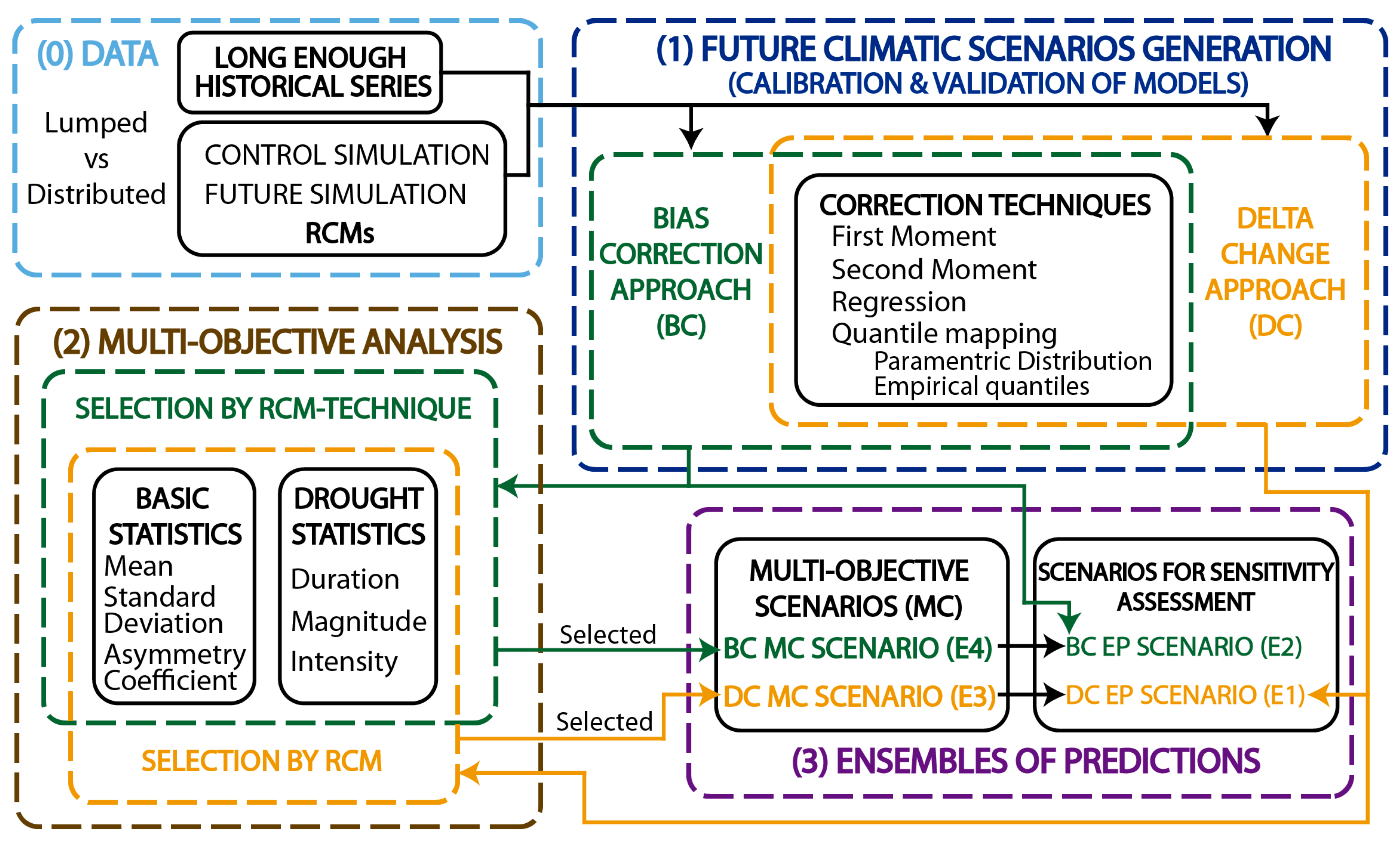
The steps of the proposed methodology to generate potential monthly future climate scenarios (precipitation and temperature) are represented in Figure 1. This includes the analysis of data and generation of future individual projections, a multi-objective analysis to identify inferior models, and different ensembles of predictions (described in Section 2.1, Section 2.2, and Section 2.3, respectively).
2.1. Generation of Future Individual Projections
An analysis of historical data and RCM simulations allows for identifying the necessity of applying statistical correction techniques to generate future scenarios. These techniques can be employed under two different approaches:
- (1)
- For each RCM model, we can represent the differences between the statistics (basic and drought statistics) of the control scenarios simulations and the “historical” values. These usually reveal significant bias, which justifies correcting them. The set of techniques to address this issue are known as bias correction approaches, since they apply a perturbation to the control series with the aim of forcing some of their statistics to get closer to the historical ones. In order to generate future series, they assume that the bias between the statistics of real data and model scenarios (control scenarios) will remain invariant into the future (e.g., [22,32]).
- (2)
- We can also represent and analyse the relative differences between control and future scenario statistics for the climatic model simulation for specific emission scenarios. Based on this information, future scenarios can be also generated by assuming that the RCMs provide accurate assessment of the relative changes in the statistics between present and future scenarios, but that they do not adequately assess the absolute values. These approaches, known as delta change solutions, use the relative difference in the statistics of control and future simulations to create a perturbation in the historical series, in accordance with these estimated changes (e.g., [25,26,27]).
Both approaches, bias correction and delta change, use the same time series (historical and control and future simulation from RCMs) to generate future climatic scenarios. In the bias correction approach, a transformation function is calibrated to modify the RCM control series, in order to obtain a corrected one whose statistics are similar to the historical ones. The calibrated correction function is applied to the future RCM simulation series to generate potential future scenarios. In the delta change approach, the transformation function is defined, taking into account the difference between future and control RCM simulations. They assume that the changes described by these transformation functions can be applied directly to the historical series to obtain potential future series. For both conceptual approaches, bias correction models and delta change solutions, we intend to test several statistical techniques with various degrees of complexity and accuracy that intend to preserve different statistics: correction of first- and second-order moments, regression approach, and QM, which are described below.
In the first-moment correction techniques, the transformation function only intends to provide a good approximation to the mean values. It is the simplest correction technique and has been extensively used for delta change [33] and bias correction [34] approaches. The second-moment correction technique is focused on the approximation of the mean and standard deviation to define the transformation function. We will apply the transformation function proposed by Pulido-Velazquez et al. [25]. The regression technique defines the transformation function by adjusting a regression function. Usually, a linear function can provide reliable results in the adjustment. This technique has been extensively applied using the bias correction approach (e.g., [35,36]). The QM is another correction technique commonly employed. The transformation is elaborated using the cumulative distribution function of the series. In this study, we will consider two QM techniques [37]: the distribution-derived transformations and empirical quantiles. The two techniques were applied using the qmap package developed by Gudmundsson et al. [37]. We will use the Bernoulli–gamma distribution to adjust precipitation data and the normal distribution for temperature series. The cumulative distribution function is approximated using tables of empirical percentiles, while values between the percentiles are approximated using linear interpolation in the case of empirical quantiles. Table 1 shows a brief summary of advantages and disadvantages of each correction technique.
In the bias correction approaches, a correction function will be calibrated to modify the control series to make the statistics of the new corrected series equal or similar to the historical ones. Since the bias correction is focused on the statistics of the series, we need to use long-enough historical and control series with invariant statistics, in order to be representative of the system climate. In cases in which these historical series can be divided into two long-enough series, one should be employed for the calibration and the other for the validation. It can be achieved through a “traditional split sample test” or a “differential split sample test” [38]. The first has earlier been used to evaluate bias correction methods for stationary conditions [39,40], while the second is used for non-stationary conditions [41]. If the series are not long enough, they might include drought or wet periods that modify the statistics of the series, making them not representative of the climate. In those cases, we need to assume the hypotheses of climate stationarity, the statistic of the representative series being invariant. In this case, the validation is not possible, and we need to assume that those inferiors in calibration would also be inferiors in a hypothetical validation. The adopted calibrated bias model will be applied to the future series to generate the corrected future scenarios.
We also analyse the statistics of the corrected series (corrected control and corrected future in the bias correction approach and future series generated by perturbation of the historical series in the delta change approach) in order to discuss and draw conclusions about the pros and cons of each statistical technique applied under different conceptual approaches.
We analyse not only classic but also drought statistics (duration, magnitude, and intensity) [42,43]. The Standard Precipitation index (SPI) was adopted to perform the drought analysis [44,45]. From the SPI series, the statistics were obtained by applying run theory [46,47]. Note that the probability of occurrence of precipitation for the SPI calculation, in the control and future simulations, was obtained using parameters calibrated from the observed series, in order to perform an appropriate comparison [9].
2.2. Multi-Objective Analysis of the Main Statistics (Basic and Drought Statistics)
A multi-objective analysis based on the goodness-of-fit to some statistics is proposed to identify the approaches that provide more reliable approximations to basic (mean, standard deviation, and asymmetry coefficient) and drought statistics (duration, magnitude, and intensity). The criteria employed to identify the inferior approaches is the next one: An approach is inferior if any other approach provides approximations significantly better for all the cited statistics (basic and drought statistics). In this analysis of the goodness-of-fit, we do not provide a higher relevance to any of the selected statistics. A homogeneous criteria (threshold) has been adopted to consider an approach significantly better than others with respect to a specific statistic. It is defined by a maximum value of the relative difference with respect to the historical statistic. This maximum threshold will be discussed in the application to the case study.
It allows discrimination of the inferior RCMs (in delta change solutions) and combinations of RCM models and correction techniques (in bias correction approaches). Note that in bias correction approaches, each technique generates a corrected control simulation, whose statistics can be compared with the historical ones, and, therefore, the goodness-of-fit for each technique can be assessed. However, delta change approaches do not generate corrected control series and the goodness-of-fit with respect to the historical statistics can only be assessed for the RCMs and not for the correction techniques.
A multi-objective analysis, somewhat similar to the one proposed here, was performed in an earlier study of an aquifer, but it was focused only on basic statistics (mean, standard deviation, and asymmetry coefficient) [26] of “delta change” solutions for two different corrections (first and second moment corrections). It aimed to identify reliable RCM models in terms of goodness-of-fit for the first and second statistics of the control scenario simulations of the historical data. The inferior RCM models (in terms of goodness-of-fit) were identified (“dominated solutions”, using the terminology of multiple-objective analysis) and eliminated. In this way, a model is eliminated if any other RCM model provides a more accurate approximation for all the cited historical statistics. In the present study, we propose a more general and complete multi-objective analysis, in which drought statistics (duration, magnitude, and intensity) are also included in the selection objective.
The application is also extended to consider bias correction approaches. This allows us to identify the best combination of RCM models and bias correction technique, in terms of the goodness-of-fit of the corrected control scenarios to the main statistics of the historical data. These multi-objective analyses should be performed in accordance with the results obtained when validating the correction model. Nevertheless, if the information cannot be divided into two long-enough series representative of the climate whose statistics are nearly invariant, we cannot perform, explicitly, a validation of the correction model. In these cases, assuming that the statistics of any long-enough period remain invariant, the calibration implicitly could be considered validated, due to the fact that the same results would be obtained under this hypothesis for any other period representatives of the climate conditions. Therefore, in these cases, the results of the calibration periods should be used to perform the multi-objective analyses.
2.3. Ensembles of Predictions to Define More Representative Future Climate Scenarios
We will study different options to define ensemble of potential future series from the results obtained in the multi-objective analysis. Some authors suggest that the ensembles of predictions produce more robust climate projections than those based on a single model [31]. We compare equifeasible solutions (considering all the RCMs simulations) and non-equifeasible solutions (considering only those RCMs, or combination of RCMs and techniques that are not inferior according to the multi-objective analysis).
Two ensemble scenarios were defined by combining, as equifeasible members, all the future series (that correspond to different RCMs simulations) generated by applying delta change (scenario E1) or bias correction (scenario E2) approaches. Note that, in the equifeasible ensembles, the number of members employed to define the future scenarios can be obtained by multiplying the number of RCMs and the number of techniques. Two other options were defined by combining only the uneliminated models (E3) (in delta change approach) or the uneliminated combinations of models and correction techniques (E4) (bias correction techniques), assuming that we do not trust the eliminated ones. As we already commented on in the previous section, in the delta change approaches, we eliminate RCM simulations, instead of series obtained by the combinations of RCM and correction technique. Therefore, when we eliminate an RCM simulation, we remove all the series generated with this RCM by applying different correction techniques. This will allow us to perform a sensitivity analysis of the goodness-of-fit of the future ensemble scenarios generated with or without any previous selection. From a methodological point of view, the proposed ensembles (E3 and E4) defined with the uneliminated models are based exclusively in those that provide better approximations of both basic and drought statistics.
The sensitivity of the solutions to the spatial scale has been also analysed for the selected case study. The Alto Genil Basin (southern Spain) extends over a wide range of altitudes and may, therefore, produce greater spatial variability with respect to the impacts of climate change on precipitation [48]. The distributed approaches are defined by applying the correction techniques (Section 2.1) to generate the future series in each cell by using the historical and RCM series available for the cell. The multi-objective analyses (Section 2.2) in the distributed approaches is defined by using, for each statistic, the weighted average for all the cells in the domain (taking into account the surface area of each) of the square relative differences, with respect to the historical one. The final ensemble of predictions obtained for the distributed approaches (Section 2.3) allows us to analyse the spatial heterogeneity of the climate change impacts. We will also analyse the sensitivity of the overall results obtained at catchment scale from using a lumped or a distributed procedure.
3. Study Area: Description and Available Data
3.1. Location and Description of the Alto Genil Basin
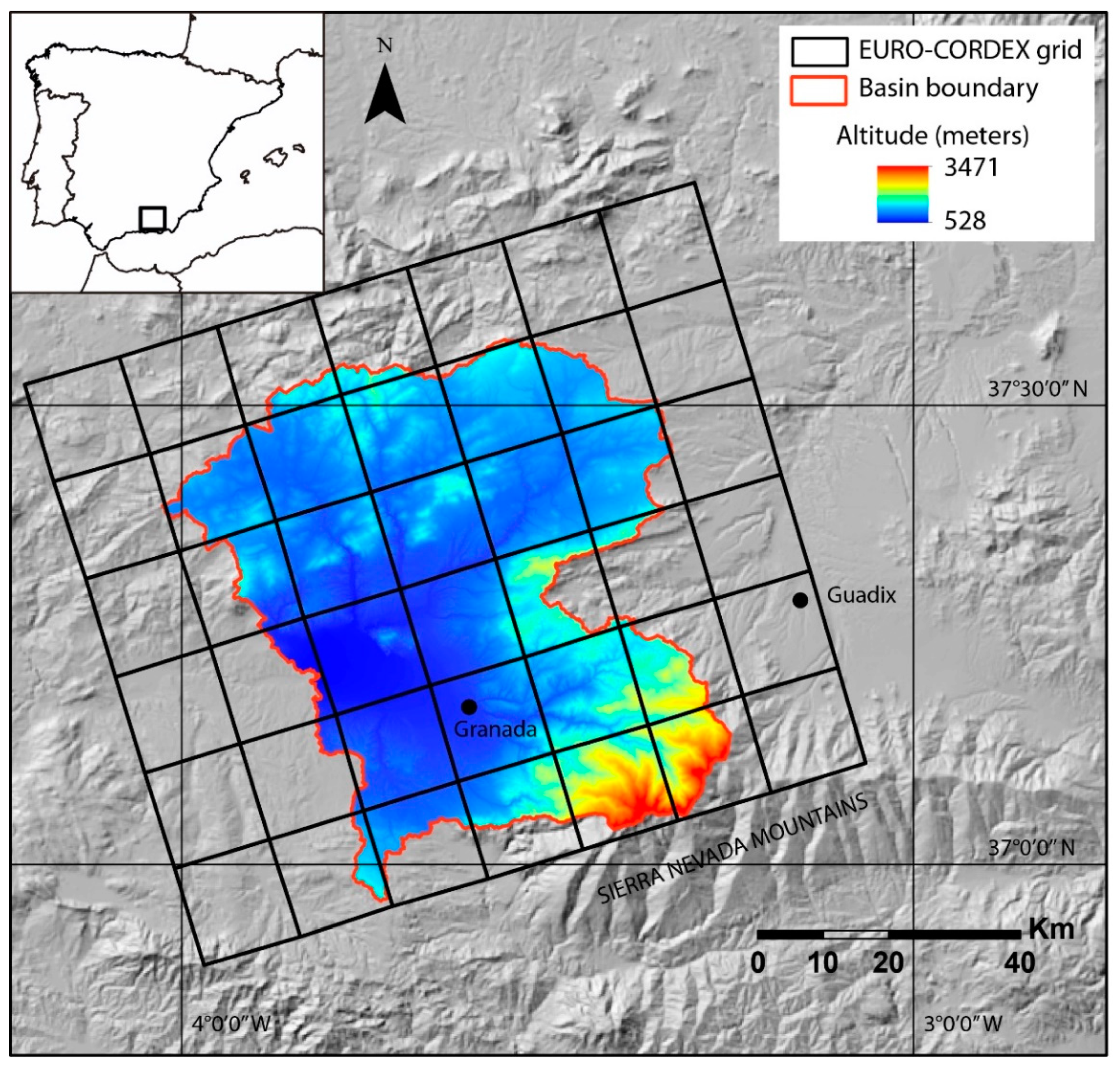
The study basin has an area of 2596 km², and it is situated in the south of Spain (see Figure 2). The basin varies substantially in elevation, from 528 m to 3471 m. The main river of the basin is the river Genil, which is the most important in the province of Granada, and one of the most important in Andalusia. The main contributions to the river come from Sierra Nevada Mountains in the melt season. The spatial resolution applied to perform a distributed approach is defined by the grid represented in Figure 2, in which the cell size is 12.5 km.
3.2. Historical Climate Data
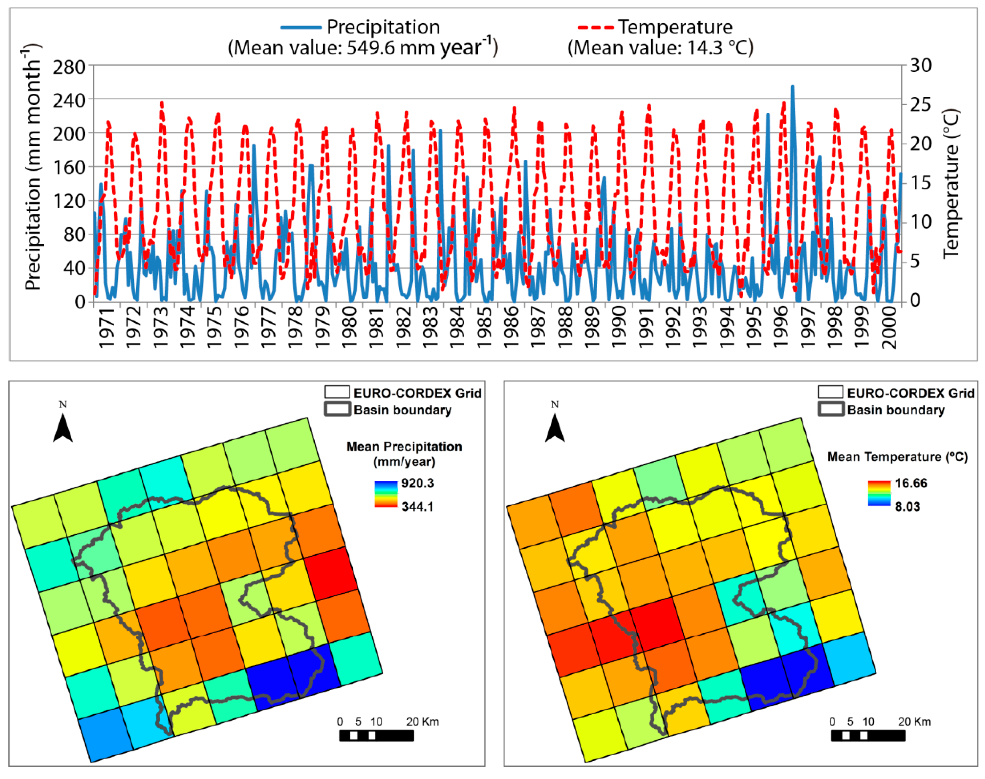
We used historical data provided by the Spain02 project [49,50] for the period 1971–2000. It includes daily temperature and precipitation estimates from observations (around 2500 quality-control stations) of the Spanish Meteorological Agency. An assessment of the validation of some Spanish datasets (including Spain02) was recently made by Quintana-Seguí et al. [51]. We used version 4 (v4) of the Spain02 project dataset (http://www.meteo.unican.es/en/datasets/spain02). The project uses the same grid as the EURO-CORDEX project [52] (see Figure 2) with a spatial resolution of 0.11° (approximately 12.5 km). The Spain02 dataset has already been employed in many research studies [53,54]. Figure 3 shows the lumped historical monthly temperature and precipitation for the catchment and the distributed mean temperature and precipitation. The areas of higher elevation (see Figure 2) produce higher precipitation and lower temperatures.
3.3. Climate Model Simulation Data. Control and Future Scenarios
The most pessimistic emission scenario of the CORDEX project [52] was considered (RCP8.5). For this scenario, we analysed nine climate-change scenarios corresponding to four different GCMs. To assess potential future climate scenarios (for the period 2071–2100) we used the output series (control and future simulations available from the CORDEX EU Project) from five RCMs (CCLM4-8-17, RCA4, HIRHAM5, RACMO22E, and WRF331F) nested inside each of the GCMs considered. The RCM simulations considered are summarised in Table 2.
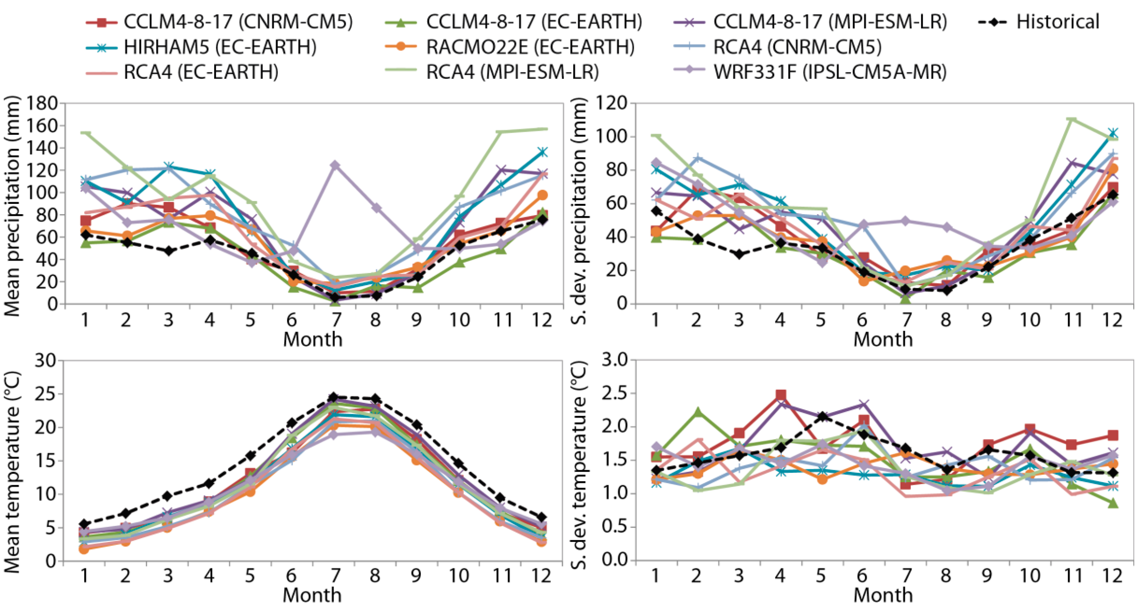
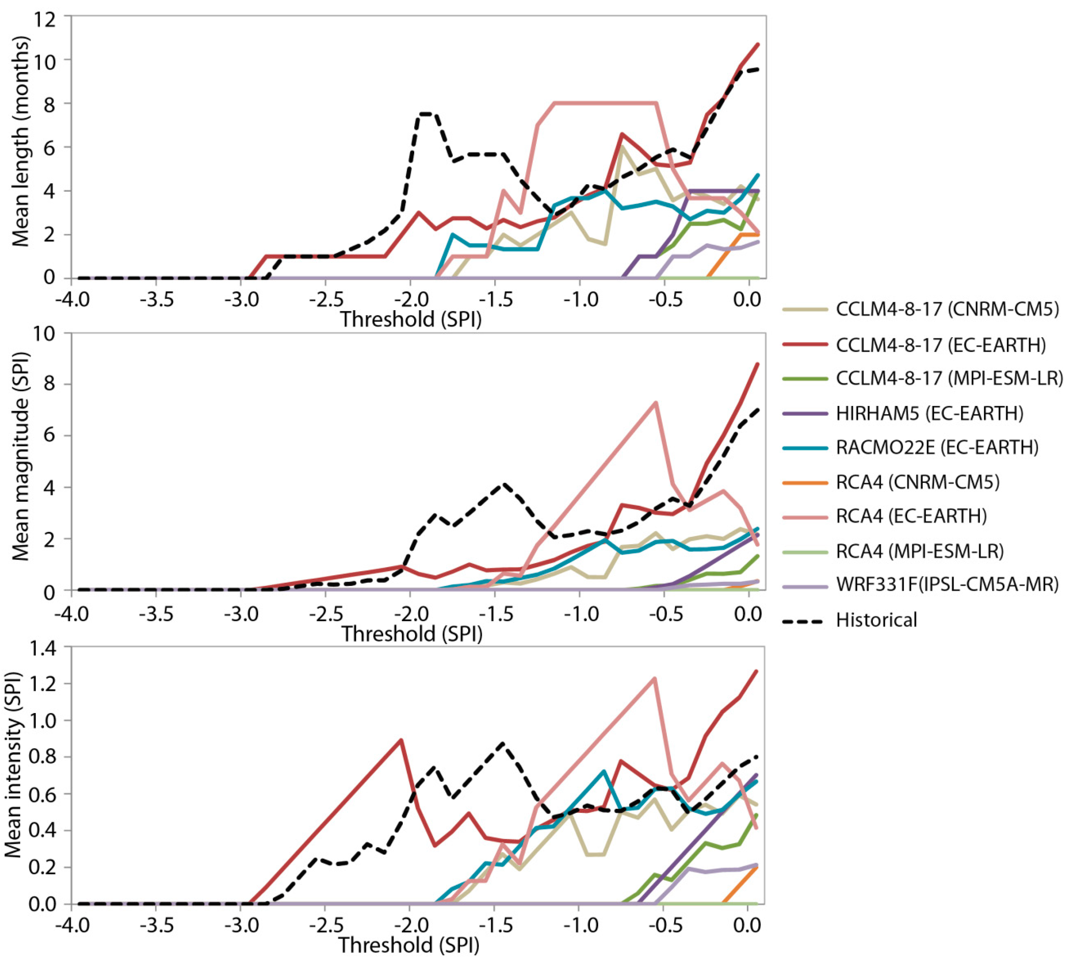
In order to show the bias between historical data and the control simulation, Figure 4 shows the monthly mean and standard deviation of the historical and control series from RCMs (precipitation and temperature) for the mean year in the reference period (1971–2000). All RCMs show significant biases with historical data for the basic statistics. The mean relative differences in precipitation are significant (54% for the mean and 36% for the standard deviation). They are lower, though also significant, for temperature (22% for the mean and 11% for the standard deviation). Figure 5 shows the drought statistics of the historical and control series of the RCM in the reference period (1971–2000). The RCM drought statistics also show significant biases with historical data.
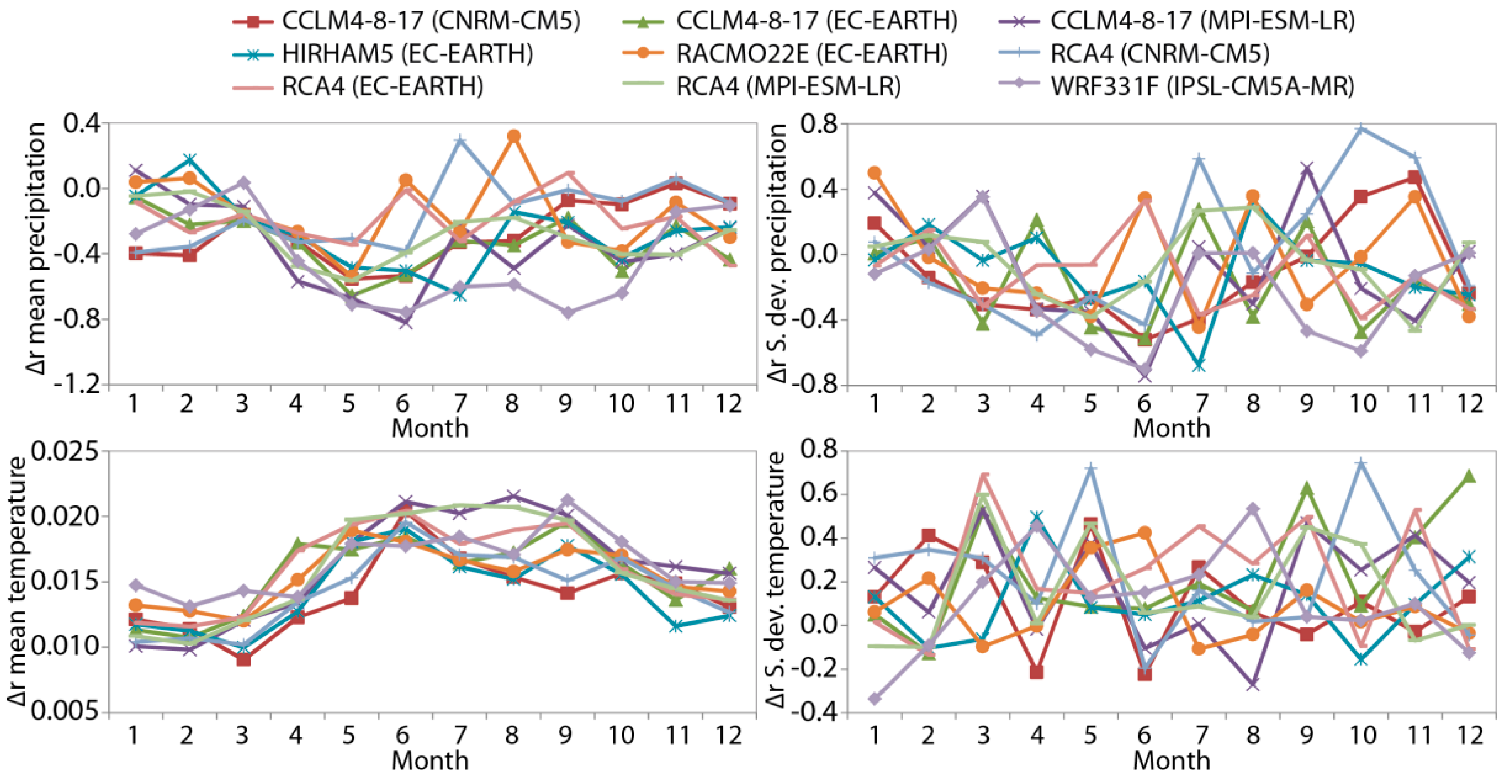
Significant bias in the basic (Figure 4) and drought (Figure 5) statistics, also pointed out by several authors in different case studies [3,23], forces us to apply a correction technique to generate future scenarios (see Section 2.1). These techniques use the relative changes between the control and future simulation to perturb the historical series, in order to generate future climatic series. Figure 6 shows the relative monthly change between mean and standard deviation of the future (2071–2100) and control (1971–2000) series (precipitation and temperature) for each RCM. This information is used directly in the delta change approach to generate the future series. However, the bias correction approach, as commented in Section 2.1, uses the changes between the historical and the control simulations. The mean relative changes in mean temperature and mean precipitation predicted by the different RCMs were −27% and 1.5%, and the mean relative changes in the standard deviation of temperature and precipitation were −9% and 16%, respectively.
4. Results and Discussion
4.1. Application of Different Correction Techniques
In order to apply statistical techniques to generate future scenarios, we assume that our 30-year period of historical data is long enough to summarise the climate conditions in our system, being similar to those obtained with any other previous historical time series. However, if we split this period in two series, the statistics of these two periods are significantly different, and we cannot perform an explicit calibration and validation of the representative climate statistics with these data. For this reason, we have used the statistics of the calibration period to assess the combinations of correction technique—RCMs under the bias correction approach and RCMs under the delta change approach, instead of using a “split sample test”.
Different correction techniques under the two considered approaches (bias correction and delta change) have been applied to the nine RCMs considered. In this section, we only present results for one of them. The results concerning all the RCMs are presented in Section 4.2 (multi-objective analysis) and Section 4.3 (ensembles of scenarios).
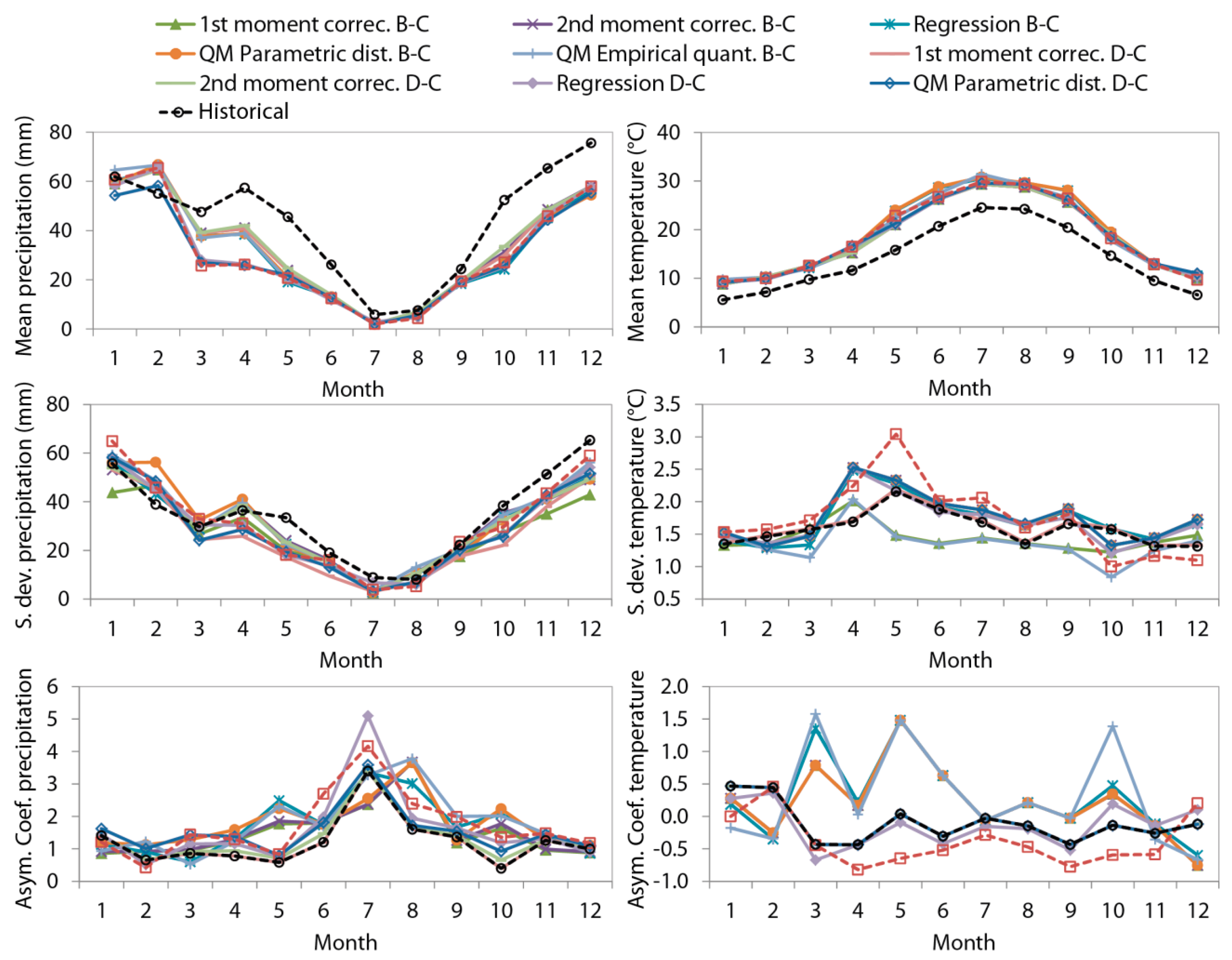
In the bias correction approach, we correct the control simulation in order to assess what combination of RCM technique provides the smallest difference compared to the historical data. If we focus on the mean, all the techniques provide accurate results. Figure 7 shows the control simulation, the corrected control simulation generated with each correction technique, and the historical data for the lumped approaches obtained for one of the nine RCMs used (HIRHAM5 RCM model nested in the EC-EARTH GCM).
The corrected control simulations for all the techniques considered reproduce, almost exactly, the monthly means of the historical data. For precipitation, there are very small differences in means for some months because the correction procedure may produce some values lower than zero, which have to be moved to zero to have physical meaning. This has been pointed out in earlier work (e.g., [25]). In terms of standard deviation, most of the techniques provide accurate results for temperature and acceptable results for precipitation, except for the first-moment correction, which maintains the same standard deviation as the control simulation. In the precipitation case, the results are not as accurate as in the temperature case because the correction procedure produces values lower than zero, which are moved to zero. For the asymmetry coefficient, QM using empirical quantiles provides the most accurate results. QM using empirical quantiles corrects this statistic, and using parametric distribution provides acceptable results. Again, these conclusions cannot be fully affirmed. With respect to the drought statistics (presented in Figure 8) for lumped approaches obtained using the HIRHAM5 RCM model nested in the EC-EARTH GCM, they still show important bias with respect to the historical droughts. As commented on in Section 1, several authors have previously pointed out that, in some cases, RCMs are not capable of reproducing the drought statistics of the observed series [14,15]. All the bias techniques provide considerable improvement in the drought statistic. However, since we are not proposing bias correction techniques that specifically correct drought statistics, we still have significant biases (see Figure 8). Nevertheless, we will apply a multi-objective analysis in order to eliminate, in the definition of potential future scenarios, the approaches that provide inferior approximations in terms of goodness-of-fit to the cited statistics.
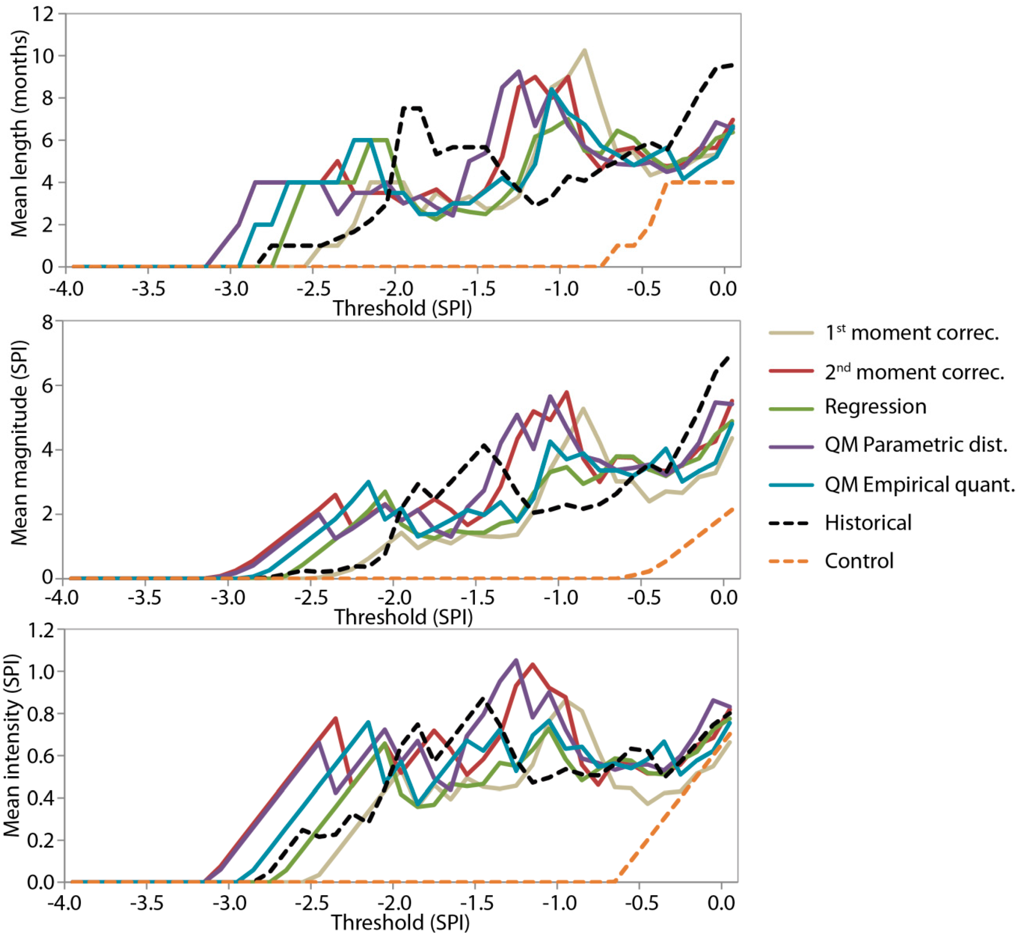
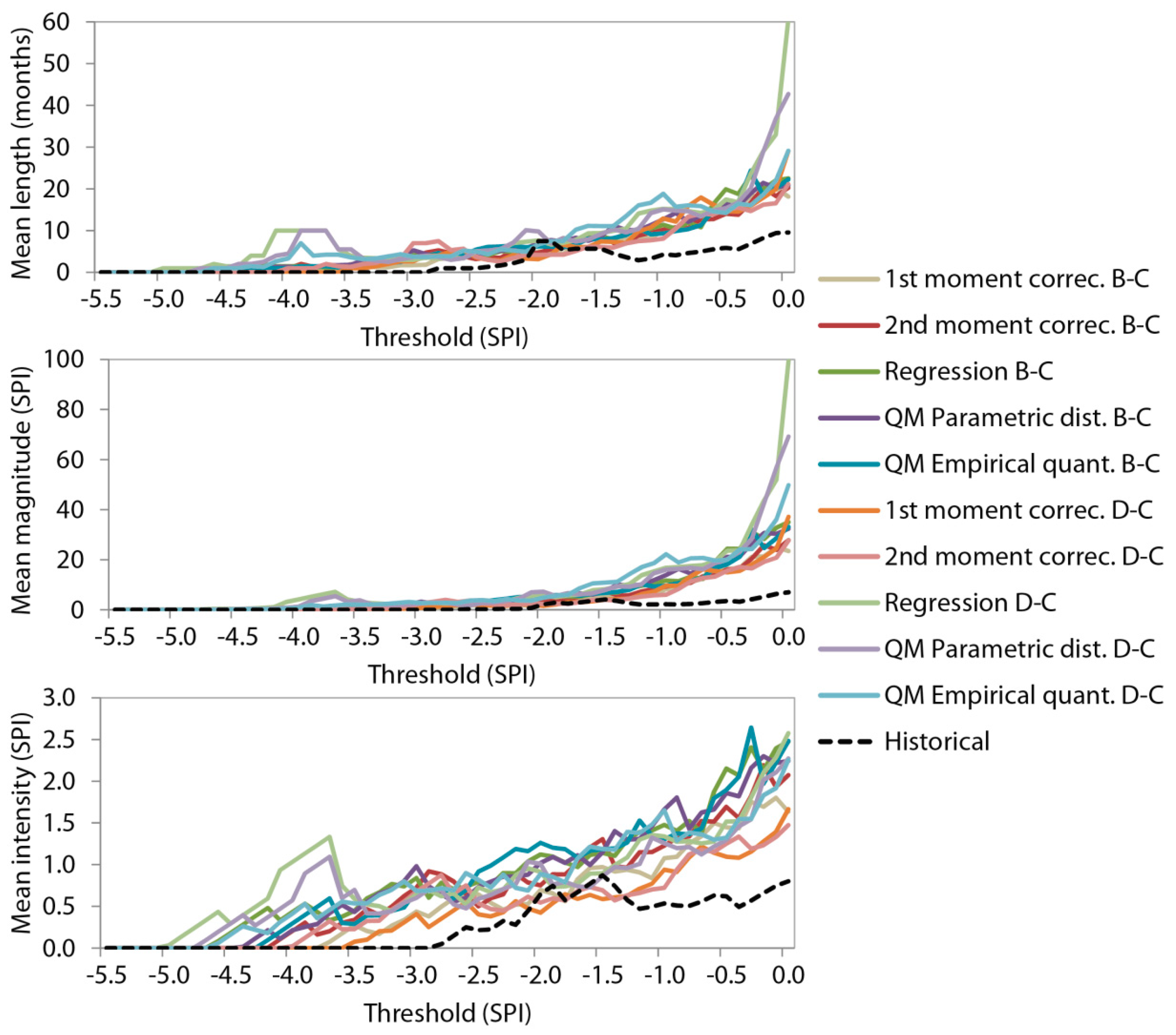
The basic and drought statistics of the future series generated (obtained using the HIRHAM5 RCM model nested in the EC-EARTH GCM) by the five correction techniques considered under the two approaches (bias correction and delta change) can be observed in Figure 9 and Figure 10, respectively. All of the generated future series provide similar monthly means, especially for temperature. First-moment correction provides the same means for the two approaches, although the generated series are different. The same happens with the second-moment correction regarding the mean and standard deviation. However, the generated series show reduced precipitation and higher temperature for all techniques and approaches. The drought analysis indicates a significant increase in duration, magnitude, and intensity of droughts (see Figure 10).
Figure 10 shows some SPI values lower than −4, which are too small, even for the Mediterranean area impacted by the extreme climate changes. In other studies, these values are commonly considered as outliers. Why do we obtain such small values? We should take into account that they are obtained from the simulation with a single specific RCM model in a long-term future horizon (2071–2100) under the most pessimistic emission scenario (RCP 8.5). On the other hand, we should also take into account that the probability of occurrence of precipitation for the SPI calculation, in the control and future simulations, was obtained using parameters calibrated from the observed series, in order to perform an appropriate comparison [9]. Nevertheless, these results show that, using a single model, we could obtain some “strange” values. For this reason, we recommend performing the analyses of potential future scenarios considering several RCMs and correction techniques. In order to reduce the uncertainty due to the RCM employed, many authors recommend using an ensemble of several approaches coming from different RCM models. In our methodology, we also propose the analyses of different ensemble solutions, which would be described for our case study in the next subsections, where we will see if we still obtain values smaller than −4.
4.2. Multi-Objective Analysis of Basic and Drought Statistics
A multi-objective analysis taking into account basic statistics (mean, standard deviation, and asymmetry coefficient) and drought statistics (duration, magnitude, and intensity) has been performed in accordance with the methodology explained in Section 2.2. Since most of the combinations of model and bias correction technique provide accurate approximations to the first and second moments, a relative error threshold was defined for each statistic to define, as inferior approaches, only those whose corrected control is significantly worse. This threshold allows us to assume certain differences in some statistics as not significant. For a given statistic, we assumed that, when the relative difference of the estimated corrected control to the historical ones is smaller than 3%, the approach is labelled accurate enough, and not considered inferior to other approaches that provide slightly better estimates. If we do not apply this threshold to the analyses of bias correction approaches, a technique producing very reliable results for certain statistics, but poor results in the others, could not be eliminated by other techniques, with reliable results in all the statistics.
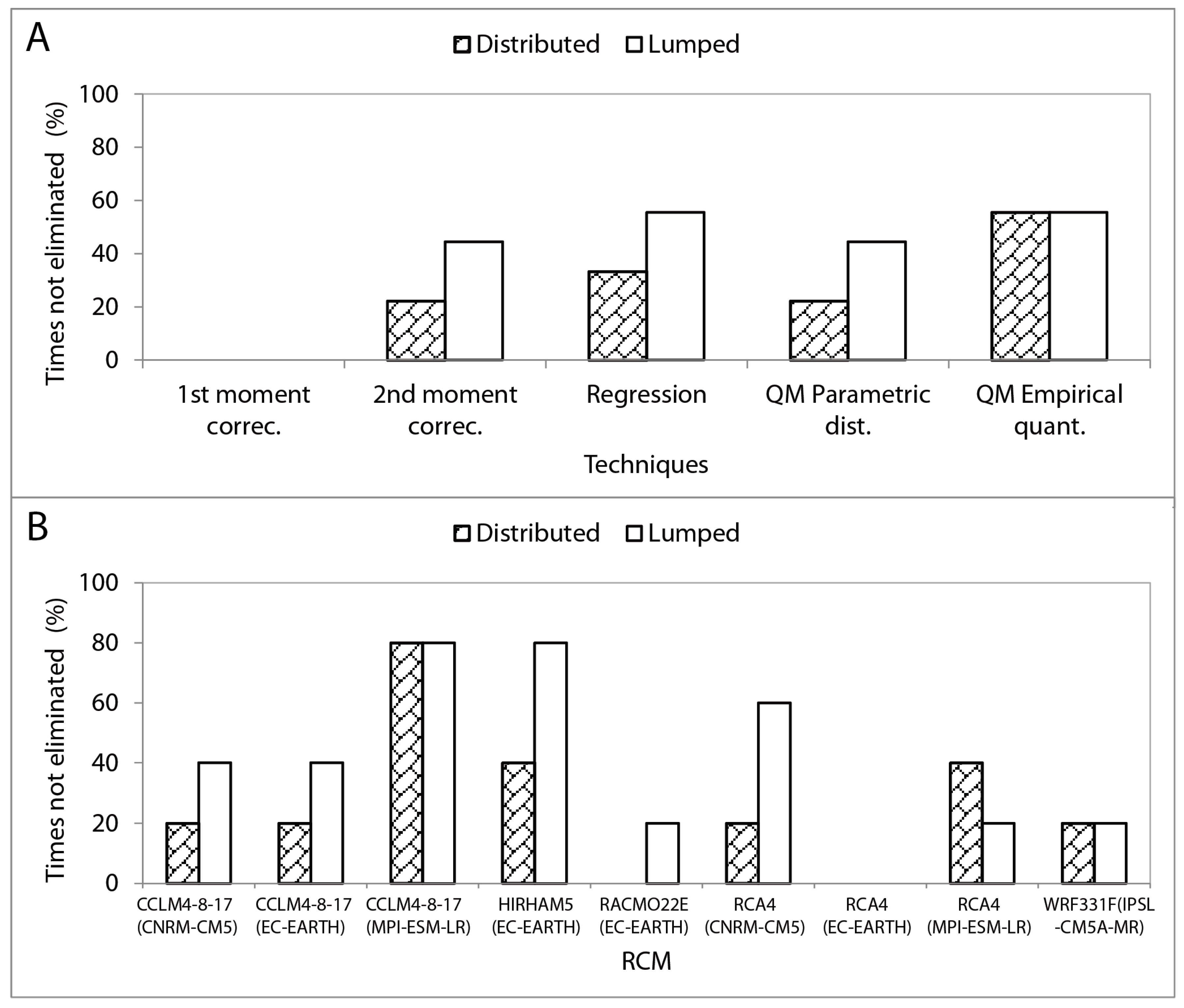
Table 3 shows the eliminated (inferior models in terms of goodness-of-fit) and uneliminated models for the delta change approaches for the lumped and distributed cases. As described in Section 2, the lumped approaches are derived from single series for the whole case study, while the distributed approaches are defined by applying the correction techniques in each cell by using the historical and RCM series available for the cell. In these distributed approaches, the multi-objective analyses is defined by using, for each statistic, the weighted average (taking into account the surface area of each) for all the cells in the domain of the square relative differences, with respect to the historical one. In the lumped case only, the RCM RCA4 nested with the GCM MPI-ESM-LR provides results inferiors to the others. In the distributed case, two models are inferior (HIRHAM5 nested to EC-EARTH and RCA4 nested to EC-EARTH). On the other hand, the multi-objective analysis allows us to identify the inferior combinations of RCM and correction technique in the bias correction approach. Table 4 shows the eliminated and uneliminated combinations of models and correction technique for the bias correction approach. The approaches obtained with the first-moment correction technique are eliminated independently of the RCM employed. The approaches coming from the model RCA4, nested to EC-EARTH, are removed independently of the correction technique employed. The data presented in Table 4 were used to elaborate Figure 11. It shows the number of times that the approaches defined with each technique or RCM are not eliminated in the multi-objective analysis under the bias correction approach. The first-moment correction technique, which is the most basic one, is always eliminated. Although it provides very accurate results in terms of the mean, its bias regarding other statistics is quite high. These simple first-moment correction approaches were also identified by other authors as the less accurate solutions [27]. The approaches obtained by regression and QM empirical quantile techniques show better agreement between historical and corrected control statistics (see Figure 7 and Figure 8), and yield a greater number of uneliminated approaches. Regarding RCMs, CCLM4-8-17 (MPI-ESM-LR) and HIRHAM5 (EC-EARTH) are the most participative models in the ensembles, though the other models have considerable participation, with the exception of RCA4 (MPI-ESM-LR) and RACMO22E (EC-EARTH).
In general, the sensitivity of the multi-objective analyses, with respect to using distributed approaches instead of lumped ones, depends on the model and the applied correction technique. Figure 11 shows that the results are not sensitive for the approaches obtained from the models MPI-ESM-LR nested to CCLM4-8-17, and IPSL-CM5A-MR nested to WRF331F. On the other hand, the approaches obtained with the correction technique “QM empirical quantile” are the only ones that are not sensitive. In general, the distributed approaches are eliminated a higher number of times than the lumped approaches, which makes sense, due to the higher complexity that supposes to fulfil the different objectives with distributed approaches.
4.3. Ensembles of Predictions to Define More Representative Future Climate Scenarios
We considered four options to define the most representative future scenarios by applying different ensembles of potential scenarios deduced from the available climate models. Two ensemble scenarios were considered by combining all future series (under different RCMs simulations and correction techniques) generated by delta change (E1) or bias correction (E2). This combination was done as equifeasible members. From the multi-objective analysis, two other combinations were defined using only the uneliminated models (E3) (in delta change approach) or the uneliminated combinations of models and correction techniques (E4) (in bias correction approach), assuming that we do not trust the eliminated ones.
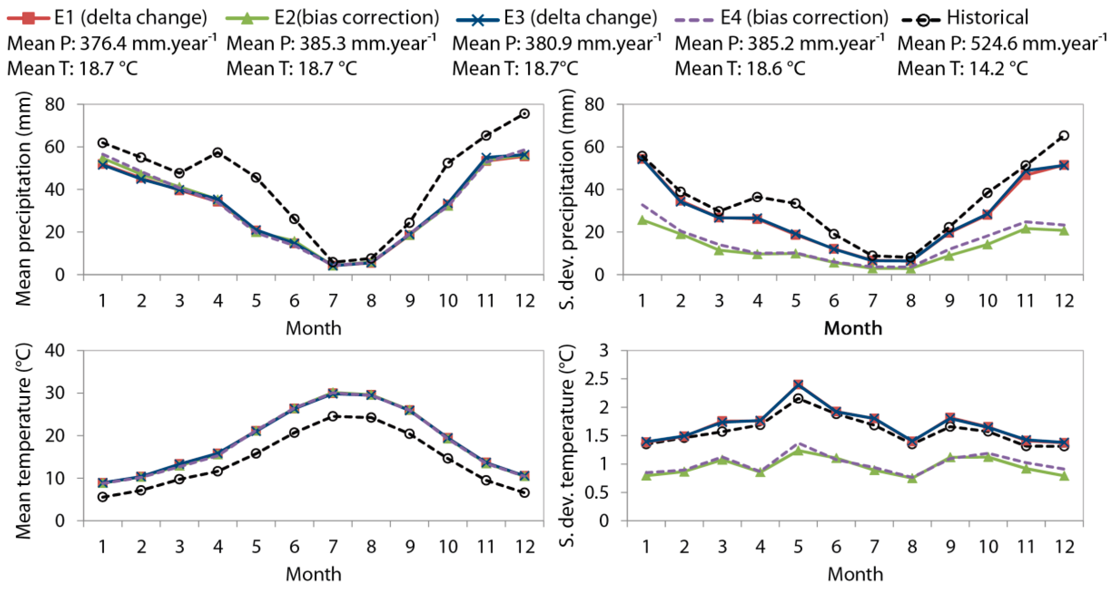
In terms of future temperature statistics, the ensemble scenarios defined with the lumped approach (Figure 12) show practically the same increment in monthly means. The standard deviation estimated using delta change approaches are quite similar to the historical, but both ensembles defined by applying bias correction show significantly lower values.
In terms of future precipitation statistics, almost the same reduction in future mean values are predicted by all the ensembles for every month (Figure 12). The standard deviation of the future precipitation predicted using the delta change approaches are more similar to the historical (as for temperature variable) than those defined by applying bias correction, whose values are significantly lower. The scenarios under the same approach provide very similar statistics.
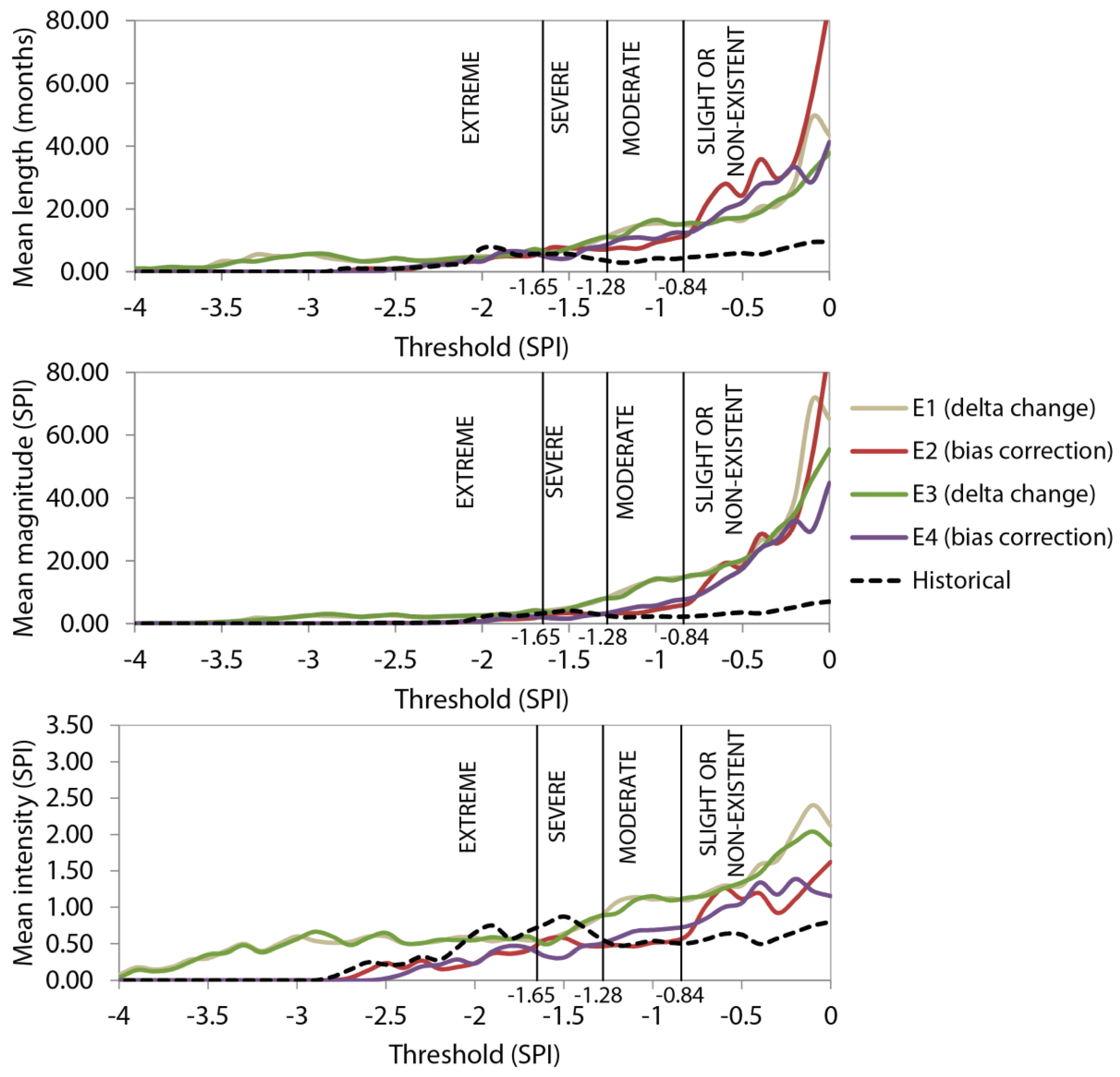
The future ensemble precipitation scenarios were analysed in terms of drought statistics (Figure 13). All four ensembles predict considerable increases in length, magnitude, and intensity of droughts as others authors pointed out for different Mediterranean zones [8,9]. Note that, although for a specific RCM model (Figure 10) we obtained some “strange” SPI values, smaller than −4 (see Section 4.1), which are usually considered as outliers, we do not obtain values smaller than −4 for any the considered ensemble scenarios in our case study. In our case study, the sensitivity of the ensemble scenarios to the multi-objective selection is low, but some differences are observed. The statistics are relatively similar in pairs considering the bias correction approach (E2 and E4 ensembles) and delta change approach (E1 and E3 ensembles). For example, for the threshold −0.84 SPI, the statistic with higher changes between the two bias correction scenarios (E2 and E4) is the magnitude with a relative change equal to 24.6%. For the two delta change ensembles (E1 and E3) the statistic with higher changes is the length with a relative change of 1.5%. Nevertheless, the results are more sensitive to the selection of bias correction or delta change approaches. The delta change approach produces more extreme droughts, reaching intensity values of around −4 SPI, while the bias correction approach does not produce droughts with SPIs higher than −2.9 (similar to the maximum historical intensity).
Nevertheless, an important con of using these ensemble scenarios, instead of multiple single projections, is that we lose information about future climate uncertainties and their potential propagation.
4.4. Sensitivity of Results to Spatial Scale
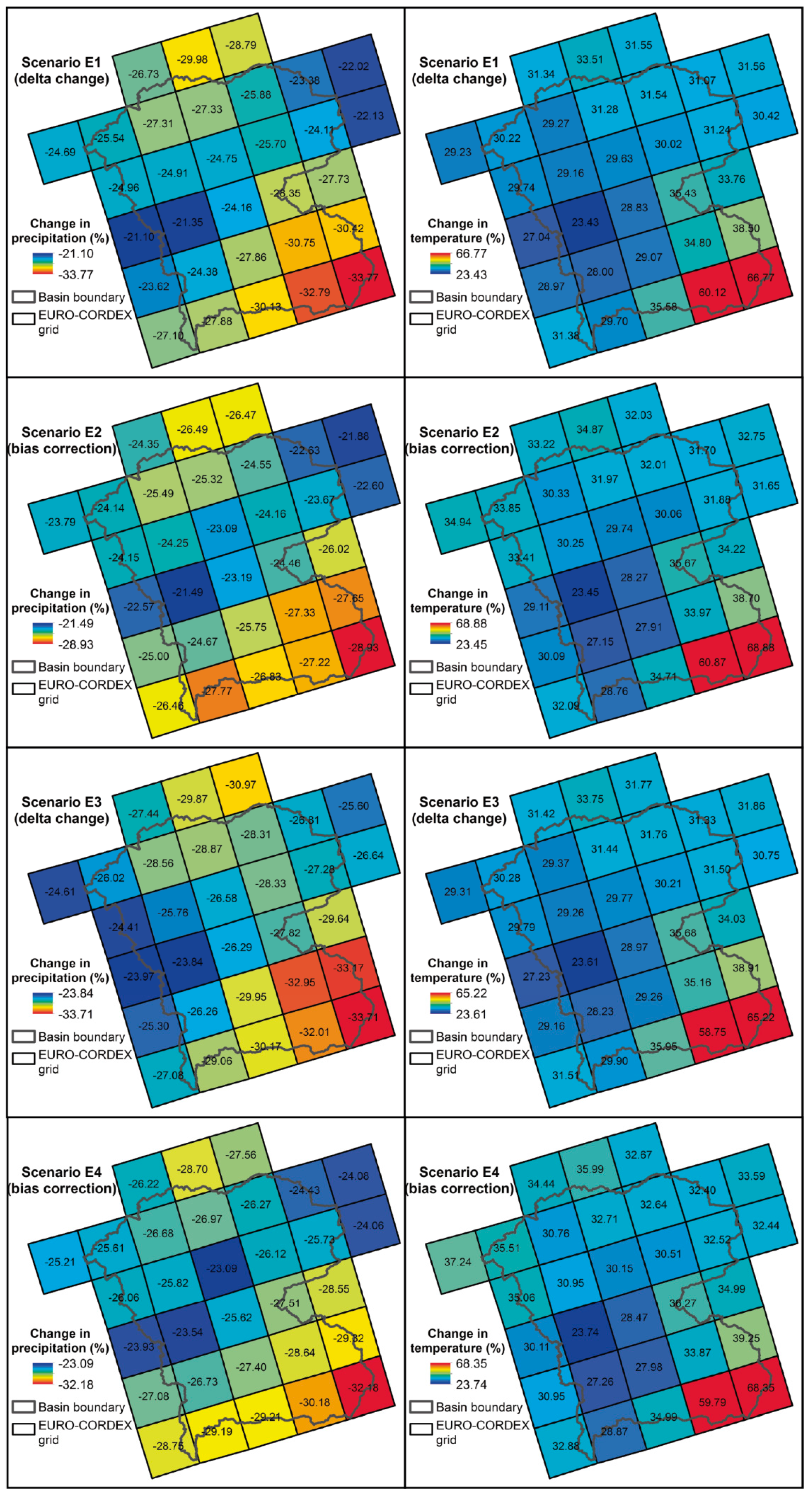
The results were also obtained in a distributed way. Figure 14 shows the spatial heterogeneity of the climate change impacts on precipitation and temperature obtained using the distributed approaches. It shows, in accordance with previous work [55], that significantly greater changes are predicted at higher altitude.
We also analysed the sensitivity of the overall results at the catchment scale calculated using the lumped or distributed procedures. Table 5 shows the mean reduction in precipitation and the overall mean rise in temperature for the four scenarios considered.
Changes in temperature are more homogeneous than in precipitation. The largest difference between the distributed and lumped cases is 1.50% for temperature in scenario E4, and 1.35% for precipitation in scenario E2. Changes in the overall mean between the various future ensemble scenarios with respect to mean historical data are small. Figure 15 shows the monthly mean relative change of the lumped case compared to the distributed case in an average year, in terms of mean and standard deviation.
The equifeasible ensembles (E1 and E2) yields the relative changes closest to zero. The maximum relative changes for the E1 scenario are −4.12%, 0.41%, −4.07%, and 0.64% for mean precipitation, mean temperature, standard deviation of precipitation, and standard deviation of temperature, respectively. For the E2 scenario, the corresponding values are −4.25%, −1.16%, −5.64%, and −3.97%. Therefore, considering an equifeasible ensemble, the differences between the lumped and distributed cases can be considered insignificant. However, in the multi-objective ensemble, these differences are considerable, since the uneliminated models and techniques are different (see Table 3 and Table 4). The maximum relative changes for the E3 scenario are 12.43%, 1.06%, 15.98%, and −3.21% for mean precipitation, mean temperature, standard deviation of precipitation, and standard deviation of temperature, respectively. The corresponding values for the E4 scenario are 11.63%, −2.33%, −28.17%, and −23.70%.
5. Limitations and Future Research Works
This work is focused on the assessment of potential future scenarios of climate change, taking into account drought statistics. From a methodological point of view, the proposed approach is an important step to define scenarios in a systematic and coherent way, taking into account meteorological drought statistics. On the other hand, the proposed statistical correction of precipitation and temperature does not preserve the energy balance when modifying the results from the RCM simulation, which could have some drawbacks as other authors previously pointed out. They reduce the uncertainty of simulations without providing a satisfactory physical justification, which can reduce the advantages of RCMs [56]. On other hand, the reduction of uncertainty could not have importance when the hydrological models have their own sources of uncertainty [57]. Nevertheless, the benefit of these new scenarios when propagating meteorological droughts to hydrological, agricultural, and operational drought have not been assessed yet. More research is required to study their propagation by using hydrological, agronomical, and management models.
In the application performed, the available data are not long enough to perform, explicitly, a calibration and a validation of the model. This work shows how to proceed in these cases, assuming stationarity of the series for an implicit validation of the model. Nevertheless, in the future, it should be also interesting to test other cases where long-enough information allows for performing an explicit validation of the model.
The proposed methodology is applied to the Alto Genil Basin (southern Spain), but could be extended to other basins in different climatic regimes and with longer periods of data, in order to draw more general conclusions.
6. Conclusions
In this research study, we propose a novel method to generate future potential climate scenarios to analyse meteorological droughts. It is based on a non-equifeasible ensemble of scenarios generated by correcting RCMs (using bias correction and delta change approaches), giving more weight to solutions that provide better approximations of the historical statistics identified in multi-objective analyses. We intend to provide consistent pictures of plausible future monthly scenarios, taking into account basic statistics (mean, standard deviation, and asymmetry coefficient) and drought statistics (duration, magnitude, and intensity) of the historical series and climatic model simulations. The drought statistics are obtained by applying run theory to the associated SPI series.
An appropriate approximation of these statistics may significantly influence the analysis of climate change impacts. A detailed analysis of the results obtained combining different hypotheses (correction techniques, conceptual approaches, equifeasible or non-equifeasible ensemble, spatial resolution) was performed for the Alto Genil Catchment.
All the RCMs considered in this study show important bias between control simulation series and historical series, in terms of basic and drought statistics. The correction techniques analysed in this work considerably reduce this bias. With the exception of the mean values, the statistics (basic and drought) of the generated scenarios are quite sensitive to the conceptual approach assumed for the correction (bias correction or delta change). If we only use a single model to generate the potential future scenarios, we might obtain some “strange” results (for example, SPI values smaller than −4) which do not appear when we use an ensemble of approaches based on different models. In order to reduce the uncertainty due to the RCM employed, several approaches coming from different RCM models should be considered. We propose the analyses of different equifeasible and non-equifeasible ensemble solutions based on a multi-objective analysis.
A multi-objective analysis based on the goodness-of-fit to some statistics is proposed to identify the approaches that provide more reliable approximations to basic (mean, standard deviation, and asymmetry coefficient) and drought statistics (duration, magnitude, and intensity). It allows discrimination of the inferior RCMs (in delta change solutions) and combinations of RCM models and correction techniques (in bias correction approaches). The approaches obtained with the first-moment correction technique, which is the most basic one, are always eliminated. Although it provides very accurate results in terms of the mean, its bias regarding other statistics is quite high. The approaches obtained by regression and QM empirical quantile techniques show better agreement between historical and corrected control statistics, and yield a greater number of uneliminated approaches.
In our application, we also conclude that the sensitivity to the hypothesis assumed to define the ensembles (equifeasible or non-equifeasible) is higher in the bias correction approach. Spatial heterogeneity of the climate change impacts on precipitation is high in our case study. Significantly greater changes are predicted in higher altitude areas. Nevertheless, the sensitivity of the overall results at catchment scale, obtained by applying lumped or distributed procedures to perform the calculations, is quite low. The four ensembles of projections for the future horizon 2071–2100 under the emission scenario RCP 8.5, show considerable increases in length, magnitude, and intensity of droughts. The average changes predicted using the four ensembles of scenarios for precipitation and temperature are quite similar for lumped and distributed cases. They are around −27% in precipitation and +32% in temperature.
Author Contributions
D.P.-V. and E.P.-I. conceived and designed the research; A.-J.C.-L. analysed the data and conducted the experiments. All authors contributed to writing the manuscript.
Funding
This research was partially funded by the GeoE.171.008-TACTIC project from GeoERA organization funded by European Union’s Horizon 2020 research and innovation program. It has been also partially funded by the PMAFI/06/14 project with UCAM funds.
Acknowledgments
We would like to thank the Spain02 and CORDEX projects for the data provided for this study and the R package qmap.
Conflicts of Interest
The authors declare no conflict of interest.
References
- Feyen, L.; Dankers, R. Impact of global warming on streamflow drought in Europe. J. Geophys. Res. 2009, 114, D17116. [Google Scholar] [CrossRef]
- Iglesias, A.; Garrote, L.; Flores, F.; Moneo, M. Challenges to manage the risk of water scarcity and climate change in the Mediterranean. Water Resour. Manag. 2007, 21, 227–288. [Google Scholar] [CrossRef]
- Blenkinsop, S.; Fowler, H.J. Changes in drought characteristics for Europe projected by the PRUDENCE regional climate models. Int. J. Climatol. 2007, 27, 1595–1610. [Google Scholar] [CrossRef]
- Skaugen, T.; Astrup, M.; Roald, L.A.; Førland, E. Scenarios of extreme daily precipitation for Norway under climate change. Hydrol. Res. 2004, 35, 1–13. [Google Scholar] [CrossRef]
- Mishra, A.K.; Singh, V.P. A review of drought concepts. J. Hydrol. 2010, 391, 202–216. [Google Scholar] [CrossRef]
- Mishra, A.K.; Singh, V.P. Drought modeling—A review. J. Hydrol. 2011, 403, 157–175. [Google Scholar] [CrossRef]
- Pedro-Monzonís, M.; Solera, A.; Ferrer, J.; Estrela, T.; Paredes-Arquiola, J. A review of water scarcity and drought indexes in water resources planning and management. J. Hydrol. 2015, 52, 482–493. [Google Scholar] [CrossRef]
- Lopez-Nicolas, A.; Pulido-Velazquez, M.; Macian-Sorribes, H. Economic risk assessment of drought impacts on irrigated agriculture. J. Hydrol. 2017, 550, 580–589. [Google Scholar] [CrossRef] [Green Version]
- Marcos-Garcia, P.; Lopez-Nicolas, A.; Pulido-Velazquez, M. Combined use of relative drought indices to analyze climate change impact on meteorological and hydrological droughts in a Mediterranean basin. J. Hydrol. 2017, 554, 292–305. [Google Scholar] [CrossRef]
- Herweijer, C.; Seager, R.; Cook, E. North American droughts of the mid to late nineteenth century: A history, simulation and implication for Mediaeval drought. Holocene 2006, 16, 159–171. [Google Scholar] [CrossRef]
- Seager, R.; Kushnir, Y.; Herweijer, C.; Naik, N.; Velez, J. Modeling of tropical forcing of persistent droughts and pluvials over western North America: 1856–2000. J. Clim. 2005, 18, 4065–4088. [Google Scholar] [CrossRef]
- Lloyd-Hughes, B.; Shaffrey, L.C.; Vidale, P.L.; Arnell, N.W. An evaluation of the spatiotemporal structure of large-scale European drought within the HiGEM climate model. Int. J. Climatol. 2013, 33, 2024–2035. [Google Scholar] [CrossRef]
- Zhang, X.; Tang, Q.; Liu, X.; Leng, G.; Li, Z. Soil moisture drought monitoring and forecasting using satellite and climate model data over Southwest China. J. Hydrometeorol. 2017, 18, 5–23. [Google Scholar] [CrossRef]
- Cook, B.; Miller, R.; Seager, R. Dust and sea surface temperature forcing of the 1930s “Dust Bowl” drought. Geophys. Res. Lett. 2008, 35, L08710. [Google Scholar] [CrossRef]
- Seager, R.; Burgman, R.; Kushnir, Y.; Clement, A.; Cook, E.; Naik, N.; Miller, J. Tropical Pacific forcing of North American medieval megadroughts: Testing the concept with an atmosphere model forced by coral-reconstructed SSTs. J. Clim. 2008, 21, 6175–6190. [Google Scholar] [CrossRef]
- Chen, J.; Brissette, F.P.; Leconte, R. Uncertainty of downscaling method in quantifying the impact of climate change on hydrology. J. Hydrol. 2011, 401, 190–202. [Google Scholar] [CrossRef]
- Chen, J.; Brissette, F.P.; Chaumont, D.; Braun, M. Performance and uncertainty evaluation of empirical downscaling methods in quantifying the climate change impacts on hydrology over two North American river basins. J. Hydrol. 2013, 479, 200–214. [Google Scholar] [CrossRef]
- Chen, J.; Brissette, F.P.; Leconte, R. Assessing regression-based statistical approaches for downscaling precipitation over North America. Hydrol. Process. 2014, 28, 3482–3504. [Google Scholar] [CrossRef]
- Räty, O.; Räisänen, J.; Ylhäisi, J. Evaluation of delta change and bias correction methods for future daily precipitation: Intermodal cross-validation using ENSEMBLES simulations. Clim. Dyn. 2014, 42, 2287–2303. [Google Scholar] [CrossRef]
- Sunyer, M.A.; Hundecha, Y.; Lawrence, D.; Madsen, H.; Willems, P.; Martinkova, M.; Vormoor, K.; Bürger, G.; Hanel, M.; Kriaučiuniene, J.; et al. Inter-comparison of statistical downscaling methods for projection of extreme precipitation in Europe. Hydrol. Earth Syst. Sci. 2015, 19, 1827–1847. [Google Scholar] [CrossRef] [Green Version]
- Piani, C.; Haerter, J.O.; Coppola, E. Statistical bias correction for daily precipitation in regional climate models over Europe. Theor. Appl. Clim. 2010, 99, 187–192. [Google Scholar] [CrossRef]
- Watanabe, S.; Kanae, S.; Seto, S.; Yeh, P.J.-F.; Hirabayashi, Y.; Oki, T. Intercomparison of bias-correction methods for monthly temperature and precipitation simulated by multiple climate models. J. Geophys. Res. 2012, 117, D23114. [Google Scholar] [CrossRef]
- Teutschbein, C.; Seibert, J. Bias correction of regional climate model simulations for hydrological climate-change impact studies: Review and evaluation of different methods. J. Hydrol. 2012, 456–457, 12–29. [Google Scholar] [CrossRef]
- Seaby, L.P.; Refsgaard, J.C.; Sonnenborg, T.O.; Højberg, A.L. Spatial uncertainty in bias corrected climate change projections and hydrogeological impacts. Hydrol. Process. 2015, 29, 4514–4532. [Google Scholar] [CrossRef]
- Pulido-Velazquez, D.; Garrote, L.; Andreu, J.; Martin-Carrasco, F.J.; Iglesias, A. A methodology to diagnose the effect of climate change and to identify adaptive strategies to reduce its impacts in conjunctive-use systems at basin scale. J. Hydrol. 2011, 405, 110–122. [Google Scholar] [CrossRef] [Green Version]
- Pulido-Velazquez, D.; García-Aróstegui, J.L.; Molina, J.L.; Pulido-Velázquez, M. Assessment of future groundwater recharge in semi-arid regions under climate change scenarios (Serral-Salinas aquifer, SE Spain). Could increased rainfall variability increase the recharge rate? Hydrol. Process. 2015, 29, 828–844. [Google Scholar] [CrossRef]
- Räisänen, J.; Räty, O. Projections of daily mean temperature variability in the future: Cross-validation tests with ENSEMBLES regional climate simulations. Clim. Dyn. 2013, 41, 1553–1568. [Google Scholar] [CrossRef]
- Rupp, D.E.; Abatzoglou, J.T.; Hegewisch, K.C.; Mote, P.W. Evaluation of CMIP5 20th century climate simulations for the Pacific Northwest USA. J. Geophys. Res. Atmos. 2013, 118, 10884–10906. [Google Scholar] [CrossRef]
- Ahmadalipour, A.; Rana, A.; Moradkhani, H.; Sharma, A. Multi-criteria evaluation of CMIP5 GCMs for climate change impact analysis. Theor. Appl. Climatol. 2015, 128, 71–87. [Google Scholar] [CrossRef]
- Hashmi, M.Z.; Shamseldin, A.Y.; Melville, B.W. Statistically downscaled probabilistic multi-model ensemble projections of precipitation change in a watershed. Hydrol. Process. 2013, 27, 1021–1032. [Google Scholar] [CrossRef]
- AEMET (Spanish Meteorologial Agency). Generación de Escenarios Regionalizados de Cambio Climático Para España; Agencia Estatal de Meteorología (Ministerio de Medio Ambiente y Medio Rural y Marino): Madrid, Spain, 2009.
- Haerter, J.O.; Hagemann, S.; Moseley, C.; Piani, C. Climate model bias-correction and the role of timescales. Hydrol. Earth Syst. Sci. 2011, 15, 1065–1079. [Google Scholar] [CrossRef]
- Prudhomme, C.; Reynard, N.; Crooks, S. Downscaling of global climate models for flood frequency analysis: Where are we now? Hydrol. Process. 2002, 16, 1137–1150. [Google Scholar] [CrossRef]
- Lafon, T.; Dadson, S.; Buys, G.; Prudhomme, C. Bias correction of daily precipitation simulated by a regional climate model: A comparison of methods. Int. J. Climatol. 2013, 33, 1367–1381. [Google Scholar] [CrossRef] [Green Version]
- Hellström, C.; Chen, D.; Achberger, C.; Räisänen, J. Comparison of climate change scenarios for Sweden based on statistical and dynamical downscaling of monthly precipitation. Clim. Res. 2001, 19, 45–55. [Google Scholar] [CrossRef] [Green Version]
- Hessami, M.; Gachon, P.; Ouarda, T.; St-Hilaire, A. Automated regression-based statistical downscaling tool. Environ. Model. Softw. 2008, 23, 813–834. [Google Scholar] [CrossRef]
- Gudmundsson, L.; Bremnes, J.B.; Haugen, J.E.; Engen-Skaugen, T. Technical Note: Downscaling RCM precipitation to the station scale using statistical transformations—A comparison of methods. Hydrol. Earth Syst. Sci. 2012, 16, 3383–3390. [Google Scholar] [CrossRef]
- Klemeš, V. Operational testing of hydrological simulation models/Vérification, en conditions réelles, des modèles de simulation hydrologique. Hydrol. Sci. J. 1986, 31, 13–24. [Google Scholar] [CrossRef]
- Bennett, J.C.; Ling, F.L.N.; Graham, B.; Grose, M.R.; Corney, S.P.; White, C.J.; Holz, G.K.; Post, D.A.; Gaynor, S.M.; Bindoff, N.L. Climate Futures for Tasmania: Water and Catchments: Technical Report; Antarctic Climate & Ecosystems Cooperative Research Centre: Hobart, Tasmania, Australia, 2010. [Google Scholar]
- Terink, W.; Hurkmans, R.T.W.L.; Torfs, P.J.J.F.; Uijlenhoet, R. Evaluation of a bias correction method applied to downscaled precipitation and temperature reanalysis data for the Rhine basin. Hydrol. Earth Syst. Sci. 2010, 14, 687–703. [Google Scholar] [CrossRef] [Green Version]
- Teutschbein, C.; Seibert, J. Is bias correction of regional climate model (RCM) simulations possible for non-stationary conditions? Hydrol. Earth Syst. Sci. 2013, 17, 5061–5077. [Google Scholar] [CrossRef] [Green Version]
- McKee, T.B.; Doesken, N.J.; Kleist, J. The relationship of drought frequency and duration to time scale. In Proceedings of the Eighth Conference on Applied Climatology, Anaheim, CA, USA, 17–22 January 1993; American Meteorological Society: Boston, MA, USA, 1993. [Google Scholar]
- McKee, T.B.; Doesken, N.J.; Kleist, J. Drought monitoring with multiple timescales. In Proceedings of the Ninth Conference on Applied Climatology, Dallas, TX, USA, 15–20 January 1995; Boston American Meteorological Society: Boston, MA, USA, 1995; pp. 233–236. [Google Scholar]
- Bonaccorso, B.; Bordi, I.; Cancelliere, A.; Rossi, G.; Sutera, A. Spatial Variability of Drought: An Analysis of the SPI in Sicily. Water Resour. Manag. 2003, 17, 273–296. [Google Scholar] [CrossRef]
- Livada, I.; Assimakopoulos, V.D. Spatial and temporal analysis of drought in Greece using the Standardized Precipitation Index (SPI). Theor. Appl. Climatol. 2007, 89, 143–153. [Google Scholar] [CrossRef]
- Mishra, A.K.; Singh, V.P.; Desai, V.R. Drought characterization: A probabilistic approach. Stoch. Environ. Res. Risk Assess. 2009, 23, 41–55. [Google Scholar] [CrossRef]
- González, J.; Valdés, J.B. New drought frequency index: Definition and comparative performance analysis. Water Resour. Res. 2006, 42, W11421. [Google Scholar] [CrossRef]
- Barnett, T.P.; Adam, J.C.; Lettenmaier, D.P. Potential impacts of a warming climate on water availability in snow-dominated regions. Nature 2005, 438, 303–309. [Google Scholar] [CrossRef] [PubMed]
- Herrera, S.; Gutiérrez, J.M.; Ancell, R.; Pons, M.R.; Frías, M.D.; Fernández, J. Development and analysis of a 50-year high-resolution daily gridded precipitation dataset over Spain (Spain02). Int. J. Climatol. 2012, 32, 74–85. [Google Scholar] [CrossRef] [Green Version]
- Herrera, S.; Fernández, J.; Gutiérrez, J.M. Update of the Spain02 Gridded Observational Dataset for Euro-CORDEX evaluation: Assessing the Effect of the Interpolation Methodology. Int. J. Climatol. 2016, 36, 900–908. [Google Scholar] [CrossRef]
- Quintana-Seguí, P.; Turco, M.; Herrera, S.; Miguez-Macho, G. Validation of a new SAFRAN-based gridded precipitation product for Spain and comparisons to Spain02 and ERA-Interim. Hydrol. Earth Syst. Sci. 2017, 21, 2187–2201. [Google Scholar] [CrossRef] [Green Version]
- CORDEX PROJECT. The Coordinated Regional Climate Downscaling Experiment CORDEX. Program Sponsored by World Climate Research Program (WCRP). 2013. Available online: http://www.cordex.org/ (accessed on 8 September 2018).
- Escriva-Bou, A.; Pulido-Velazquez, M.; Pulido-Velazquez, D. The Economic Value of Adaptive Strategies to Global Change for Water Management in Spain’s Jucar Basin. J. Water Resour. Pl. Manag. 2016, 143, 04017005. [Google Scholar] [CrossRef]
- Fernandez-Montes, S.; Rodrigo, F.S. Trends in surface air temperatures, precipitation and combined indices in the southeastern Iberian Peninsula (1970–2007). Clim. Res. 2015, 63, 43–60. [Google Scholar] [CrossRef]
- Pepin, N.C.; Lundquist, J.D. Temperature trends at high elevations: Patterns across the globe. Geophys. Res. Lett. 2008, 35, L14701. [Google Scholar] [CrossRef]
- Ehret, U.; Zehe, E.; Wulfmeyer, V.; Warrach-Sagi, K.; Liebert, J. HESS Opinions “Should we apply bias correction to global and regional climate model data?”. Hydrol. Earth Syst. Sci. 2012, 16, 3391–3404. [Google Scholar] [CrossRef]
- Muerth, M.J.; Gauvin St-Denis, B.; Ricard, S.; Velázquez, J.A.; Schmid, J.; Minville, M.; Caya, D.; Chaumont, D.; Ludwig, R.; Turcotte, R. On the need for bias correction in regional climate scenarios to assess climate change impacts on river runoff. Hydrol. Earth. Syst. Sci. 2013, 17, 1189–1204. [Google Scholar] [CrossRef] [Green Version]
Figure 1.
Flow chart of the proposed methodology.

Figure 2.
Location of the case study.

Figure 3.
Historical precipitation and temperature in Alto Genil basin. Above: Monthly precipitation and temperature time series. Below: Spatial distribution of mean precipitation and temperature.
Figure 3.
Historical precipitation and temperature in Alto Genil basin. Above: Monthly precipitation and temperature time series. Below: Spatial distribution of mean precipitation and temperature.

Figure 4.
Monthly mean and standard deviation for the historical and control series (precipitation and temperature) for the mean year in the period 1971–2000—lumped approaches.
Figure 4.
Monthly mean and standard deviation for the historical and control series (precipitation and temperature) for the mean year in the period 1971–2000—lumped approaches.

Figure 5.
Drought statistics for the historical and control series in the period 1971–2000—lumped approaches.
Figure 5.
Drought statistics for the historical and control series in the period 1971–2000—lumped approaches.

Figure 6.
Dimensionless relative monthly change in mean and standard deviation of the future P and T series (2071–2100) with respect to the control series (1971–2000)—lumped approaches. Relative changes calculated as (F − C)/C where F stands for future model projections and C control model simulations.

Figure 7.
Mean, standard deviation, and asymmetry coefficients of the corrected control scenario (1971–2000) for precipitation (left column) and temperature (right column). Average year for HIRHAM5 RCM model nested inside EC-EARTH GCM—lumped approaches.
Figure 7.
Mean, standard deviation, and asymmetry coefficients of the corrected control scenario (1971–2000) for precipitation (left column) and temperature (right column). Average year for HIRHAM5 RCM model nested inside EC-EARTH GCM—lumped approaches.

Figure 8.
Drought statistics of the corrected precipitation control scenario (1971–2000) for the HIRHAM5 RCM model nested inside EC-EARTHGCM—lumped approaches.
Figure 8.
Drought statistics of the corrected precipitation control scenario (1971–2000) for the HIRHAM5 RCM model nested inside EC-EARTHGCM—lumped approaches.

Figure 9.
Mean, standard deviation and asymmetry coefficients of future precipitation (left column) and temperature series (right column). Average year for HIRHAM5 RCM model nested inside EC-EARTH GCM—lumped approaches.
Figure 9.
Mean, standard deviation and asymmetry coefficients of future precipitation (left column) and temperature series (right column). Average year for HIRHAM5 RCM model nested inside EC-EARTH GCM—lumped approaches.

Figure 10.
Drought statistics of future precipitation series for the HIRHAM5 RCM model nested inside EC-EARTH GCM—lumped approaches.
Figure 10.
Drought statistics of future precipitation series for the HIRHAM5 RCM model nested inside EC-EARTH GCM—lumped approaches.

Figure 11.
(A) Times that the techniques are not eliminated in the multi-objective analysis (bias correction approach); (B) Times that the RCMs are not eliminated in the multi-objective analysis (bias correction change approach).
Figure 11.
(A) Times that the techniques are not eliminated in the multi-objective analysis (bias correction approach); (B) Times that the RCMs are not eliminated in the multi-objective analysis (bias correction change approach).

Figure 12.
Mean and standard deviation of future precipitation and temperature series obtained by the four ensemble options (E1, E2, E3, and E4)—lumped approaches.
Figure 12.
Mean and standard deviation of future precipitation and temperature series obtained by the four ensemble options (E1, E2, E3, and E4)—lumped approaches.

Figure 13.
Drought statistics of future precipitation series obtained by the four ensemble options (E1, E2, E3, and E4)—lumped approaches.
Figure 13.
Drought statistics of future precipitation series obtained by the four ensemble options (E1, E2, E3, and E4)—lumped approaches.

Figure 14.
Spatial distribution of the mean relative change (expressed in %) in precipitation and temperature obtained by the four ensemble options (E1, E2, E3, and E4)—distributed approaches.
Figure 14.
Spatial distribution of the mean relative change (expressed in %) in precipitation and temperature obtained by the four ensemble options (E1, E2, E3, and E4)—distributed approaches.

Figure 15.
Monthly differences in mean and standard deviation in an average year between distributed (D) and lumped (L) approaches ((L − D)/D) × 100) for the four ensembles scenarios (E1, E2, E3 and E4).
Figure 15.
Monthly differences in mean and standard deviation in an average year between distributed (D) and lumped (L) approaches ((L − D)/D) × 100) for the four ensembles scenarios (E1, E2, E3 and E4).


Table 1.
Summary of advantages and disadvantages of each correction technique (P stands for precipitation).
Table 1.
Summary of advantages and disadvantages of each correction technique (P stands for precipitation).
| Correction Technique | Pros | Cons |
|---|---|---|
| First-moment correction | - Does not generate negative values for P | - Only preserve the mean |
| Second-moment correction | - Preserve mean and standard deviation | - Generates some negative values for P |
| Regression | - Allow to use different regression models - Preserve mean and standard deviation | - Generates some negative values for P |
| Quantile mapping | - Preserve mean and standard deviation - No generates negative values of P - Variety of methods (theoretical distribution, parametric, non-parametric, empirical, splines) | - Required more complex transformations (application to the probability distribution of data) |
Table 2.
Regional climatic models (RCMs) and global climate models (GCMs) considered.
| GCM | CNRM-CM5 | EC-EARTH | MPI-ESM-LR | IPSL-CM5A-MR | |
| RCM | |||||
| CCLM4-8-17 | X | X | X | ||
| RCA4 | X | X | X | ||
| HIRHAM5 | X | ||||
| RACMO22E | X | ||||
| WRF331F | X | ||||
Table 3.
Eliminated and uneliminated models in the multi-objective analysis of the delta change approaches for the lumped and distributed cases.
Table 3.
Eliminated and uneliminated models in the multi-objective analysis of the delta change approaches for the lumped and distributed cases.
| RCM | GCM | Eliminated | |
|---|---|---|---|
| Lumped Cases | Distributed Case | ||
| CCLM4-8-17 | CNRM-CM5 | NO | NO |
| CCLM4-8-17 | EC-EARTH | NO | NO |
| CCLM4-8-17 | MPI-ESM-LR | NO | NO |
| HIRHAM5 | EC-EARTH | NO | YES |
| RACMO22E | EC-EARTH | NO | NO |
| RCA4 | CNRM-CM5 | NO | NO |
| RCA4 | EC-EARTH | NO | YES |
| RCA4 | MPI-ESM-LR | YES | NO |
| WRF331F | IPSL-CM5A-MR | NO | NO |
| CCLM4-8-17 | CNRM-CM5 | NO | NO |
Table 4.
Eliminated and uneliminated combinations of model and bias correction technique for the lumped and distributed cases.
Table 4.
Eliminated and uneliminated combinations of model and bias correction technique for the lumped and distributed cases.
| RCM | GCM | Technique | Lumped Case | Distributed Case |
|---|---|---|---|---|
| CCLM4-8-17 | CNRM-CM5 | 1st moment correc. | YES | YES |
| CCLM4-8-18 | CNRM-CM6 | 2nd moment correc. | NO | YES |
| CCLM4-8-19 | CNRM-CM7 | Regression | YES | YES |
| CCLM4-8-20 | CNRM-CM8 | QM Parametric dist. | NO | YES |
| CCLM4-8-21 | CNRM-CM9 | QM Empirical quant. | YES | NO |
| CCLM4-8-17 | EC-EARTH | 1st moment correc. | YES | YES |
| CCLM4-8-18 | EC-EARTH | 2nd moment correc. | YES | YES |
| CCLM4-8-19 | EC-EARTH | Regression | NO | YES |
| CCLM4-8-20 | EC-EARTH | QM Parametric dist. | YES | YES |
| CCLM4-8-21 | EC-EARTH | QM Empirical quant. | NO | NO |
| CCLM4-8-17 | MPI-ESM-LR | 1st moment correc. | YES | YES |
| CCLM4-8-17 | MPI-ESM-LR | 2nd moment correc. | NO | NO |
| CCLM4-8-17 | MPI-ESM-LR | Regression | NO | NO |
| CCLM4-8-17 | MPI-ESM-LR | QM Parametric dist. | NO | NO |
| CCLM4-8-17 | MPI-ESM-LR | QM Empirical quant. | NO | NO |
| HIRHAM5 | EC-EARTH | 1st moment correc. | YES | YES |
| HIRHAM5 | EC-EARTH | 2nd moment correc. | NO | NO |
| HIRHAM5 | EC-EARTH | Regression | NO | NO |
| HIRHAM5 | EC-EARTH | QM Parametric dist. | NO | YES |
| HIRHAM5 | EC-EARTH | QM Empirical quant. | NO | YES |
| RACMO22E | EC-EARTH | 1st moment correc. | YES | YES |
| RACMO22E | EC-EARTH | 2nd moment correc. | YES | YES |
| RACMO22E | EC-EARTH | Regression | NO | YES |
| RACMO22E | EC-EARTH | QM Parametric dist. | YES | YES |
| RACMO22E | EC-EARTH | QM Empirical quant. | YES | YES |
| RCA4 | CNRM-CM5 | 1st moment correc. | YES | YES |
| RCA4 | CNRM-CM5 | 2nd moment correc. | NO | YES |
| RCA4 | CNRM-CM5 | Regression | NO | YES |
| RCA4 | CNRM-CM5 | QM Parametric dist. | YES | YES |
| RCA4 | CNRM-CM5 | QM Empirical quant. | NO | NO |
| RCA4 | EC-EARTH | 1st moment correc. | YES | YES |
| RCA4 | EC-EARTH | 2nd moment correc. | YES | YES |
| RCA4 | EC-EARTH | Regression | YES | YES |
| RCA4 | EC-EARTH | QM Parametric dist. | YES | YES |
| RCA4 | EC-EARTH | QM Empirical quant. | YES | YES |
| RCA4 | MPI-ESM-LR | 1st moment correc. | YES | YES |
| RCA4 | MPI-ESM-LR | 2nd moment correc. | YES | YES |
| RCA4 | MPI-ESM-LR | Regression | YES | NO |
| RCA4 | MPI-ESM-LR | QM Parametric dist. | NO | NO |
| RCA4 | MPI-ESM-LR | QM Empirical quant. | YES | YES |
| WRF331F | IPSL-CM5A-MR | 1st moment correc. | YES | YES |
| WRF331F | IPSL-CM5A-MR | 2nd moment correc. | YES | YES |
| WRF331F | IPSL-CM5A-MR | Regression | YES | YES |
| WRF331F | IPSL-CM5A-MR | QM Parametric dist. | YES | YES |
| WRF331F | IPSL-CM5A-MR | QM Empirical quant. | NO | NO |
Table 5.
Changes of overall mean values for precipitation and temperature scenarios compared to historical data.
Table 5.
Changes of overall mean values for precipitation and temperature scenarios compared to historical data.
| Scenario | Lumped Case | Distributed Case | ||
|---|---|---|---|---|
| P | T | P | T | |
| Absolute Changes (mm or °C) | ||||
| E1 | −147.9 | 4.5 | −142.4 | 4.5 |
| E2 | −139.0 | 4.5 | −131.9 | 4.6 |
| E3 | −143.4 | 4.5 | −149.4 | 4.5 |
| E4 | −139.1 | 4.4 | −141.9 | 4.6 |
| Relative Changes (%) | ||||
| E1 | −28.21 | 31.94 | −27.16 | 31.66 |
| E2 | −26.51 | 31.59 | −25.16 | 32.05 |
| E3 | −27.35 | 31.74 | −28.50 | 31.79 |
| E4 | −26.53 | 30.99 | −27.06 | 32.49 |
© 2018 by the authors. Licensee MDPI, Basel, Switzerland. This article is an open access article distributed under the terms and conditions of the Creative Commons Attribution (CC BY) license (http://creativecommons.org/licenses/by/4.0/).
Share and Cite
MDPI and ACS Style
Collados-Lara, A.-J.; Pulido-Velazquez, D.; Pardo-Igúzquiza, E. An Integrated Statistical Method to Generate Potential Future Climate Scenarios to Analyse Droughts. Water 2018, 10, 1224. https://doi.org/10.3390/w10091224
AMA Style
Collados-Lara A-J, Pulido-Velazquez D, Pardo-Igúzquiza E. An Integrated Statistical Method to Generate Potential Future Climate Scenarios to Analyse Droughts. Water. 2018; 10(9):1224. https://doi.org/10.3390/w10091224
Chicago/Turabian StyleCollados-Lara, Antonio-Juan, David Pulido-Velazquez, and Eulogio Pardo-Igúzquiza. 2018. "An Integrated Statistical Method to Generate Potential Future Climate Scenarios to Analyse Droughts" Water 10, no. 9: 1224. https://doi.org/10.3390/w10091224
Note that from the first issue of 2016, this journal uses article numbers instead of page numbers. See further details here.