Analysis and Prediction of Dammed Water Level in a Hydropower Reservoir Using Machine Learning and Persistence-Based Techniques

Abstract

This paper presents long- and short-term analyses and predictions of dammed water level in a hydropower reservoir. The long-term analysis was carried out by using techniques such as detrended fluctuation analysis, auto-regressive models, and persistence-based algorithms. On the other hand, the short-term analysis of the dammed water level in the hydropower reservoir was modeled as a prediction problem, where machine learning regression techniques were studied. A set of models, including different types of neural networks, Support Vector regression, or Gaussian processes was tested. Real data from a hydropower reservoir located in Galicia, Spain, qwew considered, together with predictive variables from upstream measuring stations. We show that the techniques presented in this paper offer an excellent tool for the long- and short-term analysis and prediction of dammed water level in reservoirs for hydropower purposes, especially important for the management of water resources in areas with hydrology stress, such as Spain.

1. Introduction

The use of river water resources by means of reservoirs and dams is of primary importance for energy generation, water supply, navigation, and flood control, among others [1]. Over half of the major river systems in the world have dammed reservoirs, which control or affect the river’s flow [2]. The management of water reservoirs in rivers is therefore a critical problem, including many possible tasks that depend on the specific aim of the dammed reservoir. Among these tasks, the prediction of the dammed water level in the reservoir is critical in many cases, for evaluating structural problems in dams [3], water supply and resource availability [4,5], water quality [6,7,8], bio-diversity conservation [9], navigation management [10], disaster prevention [11], and hydropower production optimization, which is the problem we are interested in this paper [12,13].

The problem of dammed water level prediction in reservoirs can be tackled by considering very different predictive variables (input data). Many authors [14,15] have considered hydro-meteorological data, but alternative input data for prediction are also available, such as images from video cameras [16] or satellite-based information [17,18], among other possibilities. Regarding the computational methods applied in dammed water level prediction problems, there have been different attempts using time series processing algorithms [19], empirical orthogonal functions [20], error correction-based forecasting [21], multivariate approaches [22], or ensemble-based algorithms [23]. However, the use of Machine Learning (ML) algorithms in this problem has been massive in the last years, including many different types of learning algorithms such as neural networks, support vector machines, and different hybrid approaches. One of the first approaches using ML algorithms for level prediction in reservoirs was presented by [24], who compared the performance of artificial neural networks and neuro-fuzzy approaches in a problem of short-term water level in two German rivers, from hydrological upstream data. Adaptive neuro-fuzzy inference algorithms were also considered by [25,26] for water level prediction in reservoirs after typhoons events. In [1], the performances of different ML algorithms such as neural networks, support vector regression, and deep learning algorithms are evaluated in a problem of reservoir operation (mainly inflow and outflow prediction) at different time scales, in the Gezhouba dam, across the Yangtze River, in China. In [27], a recurrent neural network is proposed for estimating the inflow of a reservoir from a distributed hydrological model. In addition, different hybrid ML approaches have been proposed for problems of water level prediction in reservoirs, e.g., [28], hybridized a neural network with a genetic algorithm to improve the network training. This hybrid approach was tested in a problem of dammed water level prediction at the low Han River, China. In [29], a Support Vector Regression (SVR) algorithm hybridized with a fruit fly algorithm for SVR parameter optimization is proposed. In this case, the authors tested it on a problem of river flow forecasting in Lake Urmia basin, Iran.

In this paper, we present long- and short-term analyses and predictions of dammed water level in a reservoir for hydropower generation. We evaluated the use of persistence-based techniques for long-term analysis of the dammed water level for hydropower (including Detrended Fluctuation Analysis (DFA), auto-regressive models, and pure persistence-based techniques, such as a typical year for dammed water level calculation), together with a number of ML regression techniques for short-term prediction of dammed water level at of Belesar hydropower reservoir (Miño River, Galicia, Spain). The long-term analysis was carried out directly from water level data of the reservoir. On the other hand, for the short-term analysis, the ML models used exogenous hydro-meteorological input variables measured at different stations upstream the river which feeds the reservoir, at weekly time-horizon.

The main contributions of this paper are the following:

• We show that the long-term persistence of the total amount of dammed water at Belesar reservoir has a clear yearly pattern, which supports the application of persistence-based approaches such as typical year or AR models.
• We show how ML techniques are extremely accurate in short-term prediction, involving exogenous hydro-meteorological variables.
• We evaluated the performance of a number of the ML regressors such as multi-layer perceptrons, support vector regression, extreme learning machines, or Gaussian processes in this problem of short-term prediction.
• We finally show how the seasonal pattern of dammed water is very accused in this prediction problem; thus, it can be exploited to obtain better prediction mechanisms, mainly in short-term prediction.

The rest of the paper has been structured as follows. Section 2 presents the data available for this study and all the methods applied to the analysis and prediction of the dammed water level at the objective reservoir. Section 3 presents the experimental part of the article, where the performance of the previously defined approaches is evaluated in the problem. This section also includes a discussion and analysis part, where the results obtained are detailed in connection with previous studies in the literature. Finally, Section 4 closes the paper with some ending conclusions and remarks.

2. Data and Methods

In this section, we first describe the data available for this study, and the methodology carried out, mainly the data split in train and test, and the different input variables considered. The long- and short-term algorithms considered in this study are also described in this section. For the long-term analysis of the dammed water level in the reservoir (reservoir water volume available), we used DFA, auto-regressive models, and a typical year based on persistence algorithm. The short-term analysis of the dammed water level was formulated as a weekly time-horizon prediction problem, where different ML regression techniques were evaluated, such as multi-layer perceptrons, extreme learning machines, support vector regression algorithms or Gaussian processes.

2.1. Data Description and Methodology

Belesar is a dammed water reservoir on the Miño River in Galicia (42.628889${}^{°}$ N, 7.7125${}^{°}$ W), Spain, built in 1963 [30]. Its maximum capacity is 655 hm${}^3$, with a surface of 1910 ha. Belesar reservoir was created as part of a hydropower project, together with a hydropower station. This reservoir is also used for human consumption in the zone. Figure 1 shows the reservoir location at the north-west of Spain. Dammed water level (hm${}^3$) daily data (complete 51 years) are available since the beginning of the reservoir operation, on 1 October 1963, until 30 September 2015. Note that an expansion work in the power generating section of the dam was carried out in 2011, which required the reservoir to be drained almost completely from spring to winter. We therefore skipped 2011 in this study. We considered weekly data, by averaging the daily dammed water level in weekly periods, obtaining a total of 2704 data samples. Observe that, in the long-term analysis, we only considered data from the dammed water level historic time series at Belesar. However, for short-term analysis, exogenous variables must be considered to obtain atmospheric and hydrological information to feed the ML models. This way, we also considered data from nine measuring stations located upstream Miño River and on its tributaries. Figure 2 shows the time series of weekly water level at Belesar reservoir. Figure 2a shows the complete series from 1964 to 2015. We used it to evaluate the long-term prediction and analysis methods. Figure 2b shows the time series since 2009, when data from upstream measuring stations are available. We considered in the latter dataset the results obtained in short-term prediction by the ML regression methods. The descriptive statistics for both cases (complete series and series since 2009) are shown in

Table 1. Descriptive statistics for the dependent variable (water level at Belesar reservoir) for both problems presented in this paper: long-term prediction and analysis (time series since 1964) and short-term prediction (time series since 2009).

Time Series Descriptive Statistics	Water Level Data for Short-Term Prediction Since 2009 (hm${}^3$)	Water Level Data for Long-Term Analysis Since 1964 (hm${}^3$)
Minimum	77.36	33.21
1st Quartile	225.92	244.61
Median	374.92	391.64
Mean	354.42	371.80
3rd Quartile	491.16	511.54
Maximum	560.68	653.62
Standard Deviation	147.19	161.00

.

The location of the measuring stations is also shown in Figure 1. These stations measure the height (m) and flow (m${}^3$/s) upstream and on the tributaries, and also the precipitation amount (mm), both of which account for the predictor variables. The target variable is the dammed water level at Belesar reservoir, measured in hm${}^3$. Along with this variable, another one is provided with the dam’s data: the amount of water used to generate electricity, measured in m${}^3$/s. Given that this water is taken out from the reservoir, it was considered as another input to the model. A change in the demand of electricity causes a variable decrease in the water available in the reservoir. This directly affects the levels of water stored in the reservoir in the next weeks, and, without this variable, this decrease would be impossible to be accounted for by the model.

In addition, the depth of snow accumulated and the level of snow melt were used in the months of spring to try to improve the results obtained with only hydro-meteorological variables. Given the geographical region where the rivers and reservoir are located, barely any high terrain nearby could accumulate snow during the autumn and winter months, and it could affect the levels of water in the reservoir by means of groundwater(s). The snow data were obtained from the reanalysis ERA5 model from the Climate Data Store API [31]. Given that the data of the predictors and the target variable were obtained from different sources, the starting and ending dates do not match. The reservoir data start in 1963 and stopped on 30 September 2015. In turn, the predictive data, from the measurement stations and the Climate Data Store API, start 1 January 2009 and end on 31 December 2015. To use the maximum amount of data available, the dates used in the short-term analysis of Belesar dammed water level for hydropower were considered from 1 January 2009 to 30 September 2015.

As mentioned above, the original data were on a daily basis, thus a weekly aggregation was performed both for long- and short-term analyses. This improved the representation of the differences in the changes of the level of the water stored in the reservoir; otherwise, the differences in a smaller scale of time (daily or hourly) would be too small and unstable to properly train the model. Depending on the type of variable, either an average or a sum was performed. On the precipitations and the output of the reservoir (water used for electricity production), the sum was calculated, while, for the variables that measure the level of the tributaries and the reservoir level, averages were obtained to convert them to weekly data. In the short-term case, we considered a prediction problem with a time-horizon prediction of one week; thus, in this case, the predictive variables were time delayed one week with respect to the objective variable (i.e., the values of the independent variables for the first week of 2009 were used to predict the dammed water level on the second week, and so on). Finally, note that outliers were removed in the target series, so that the models could generalize better on new unknown data that were not used in the training process. As previously explained, in 2011, an expansion work in the power generating section of the dam was carried out which required the reservoir to be drained almost completely for the greater part of the year, specifically from spring to winter. The values of all the variables (both predictive and explained) from that period were removed. After the cleaning and pre-processing of the data, there were 306 data samples for the short term experiments. A seasonal approach was also considered as part of the experimental performance of the ML algorithms considered. Firstly, the available data were split into the four seasons of the year. Then, every regression technique was trained with each corresponding seasonal dataset (data of all the years available but with only one season of the year). This way, it was possible to assess how the different models perform on each season and, accordingly, it was possible to select the best model to predict the dammed water level for spring, summer, autumn, and winter.

To analyze all the input variables effect in the ML regression techniques, different groups of input variables were used to create multiple datasets. This way, the best models could be chosen, so that they were trained with different sets of variables for each season.

Table 2. Input variables included in each of the datasets used in the experimental evaluation of the ML regression techniques for short-term analysis and prediction of dammed water level at Belesar.

Dataset	Variables Included	Number of Variables
1	Upstream and tributaries’ flow	19
2	Upstream and tributaries’ flow & Precipitations	28
3	Upstream and tributaries’ flow, Precipitations & Reservoir output	29
4	Upstream and tributaries’ flow, Precipitations, Reservoir output & Snow data	31

shows the different groups of input variables considered.

A hold-out scheme was used in all the experiments for short-term analysis and prediction with ML algorithms, with a 80/20 split, where $80\%$ of the data were used to train and $20\%$ for testing. This helped check the performance of the trained models on new unseen data. With this hold-out scheme, two datasets were created: a first dataset where the data were split randomly, each week was chosen randomly for training or testing, and a second dataset where the division was made in a temporal manner, taking the first $80\%$ of the weeks for training and the last $20\%$ for testing the models, which allowed a temporal view of the predictions even if the problem was not properly accounted for as a time series by the regression models.

2.2. Detrended Fluctuation Analysis for Long-Term Persistence Evaluation

The DFA algorithm has been recently proposed to analyze long-term persistence in time series in a number of applications [32]. It was also used in the long-term analysis of Belesar water level for hydropower generation. The DFA algorithm consists of three steps:

(1)

First, the periodic annual cycle of the time series is removed, by the procedure explained in detail in [27]. The process consists in standardizing the input time series $x_i$ of length N as follows:

$$x_i^{\prime }=\frac{x_i-{\overline{x}}_i}{{\sigma }_i},$$

(1)

where $x_i$ stands for the original time series, ${\overline{x}}_i$ represents the mean value of the time series, and ${\sigma }_i$ is its standard deviation.

(2)

Then, the time series profile $Y_j$ (integrated time series) is computed as follows:

$$Y_j=\sum _{i=1}^j{x}_i^{\prime }.$$

(2)

The profile $Y_j$ is divided into $N_s=⌊\frac{N}{s}⌋$ non-overlapping segments $Y_j^s=\left\{Y_j^k\right|1\le k\le N_s\}$ of equal length s.

For each segment $Y_j^k$, the local least squares straight-line $Z_j^k$ is calculated, which measures its local trend. As a result, a linear peace-wise function ${\tilde{Z}}_j^s$ compounding each linear fitting is obtained:

$${\tilde{Z}}_j^s=\left[\begin{array}{ccccc}{Z}_j^1& \cdots & Z_j^k& \cdots & Z_j^{N_s}\end{array}\right],$$

(3)

where the superscript s refers to the time window length used to the linear fitting of each piece.

(3)

Then, the so-called fluctuation as the root-mean-square error from this linear piece-wise function ${\tilde{Z}}_j^s$ and the profile $Y_j$ is obtained, varying the time window length s:

$$F\left(s\right)=\sqrt{\frac{1}{N}\sum _{k=1}^N{({\tilde{Z}}_j^s-Y_j^s)}^2}.$$

(4)

At the time scale range where the scaling holds, $F\left(s\right)$ increases with time window s as power law $F\left(s\right)\propto s^{\alpha }$. Thus, the fluctuation $F\left(s\right)$ versus the time scale s would be depicted as a straight line in a log-log plot. The slope of the fitted linear regression line is the scaling exponent $\alpha$, also called correlation exponent. If this coefficient $\alpha =0.5$, the time series is uncorrelated, which means there is not long-term persistence in the time series. For larger values of $\alpha$, the time series are positively long-term correlated, which also means the long-term persistence exist across the corresponding scale range.

A recent study has applied a DFA analysis for studying the long-term persistence of rainfall and streamflow in India and USA [33].

2.3. Auto-Regressive Moving Average Models

Auto-Regressive-Moving-Average (ARMA) models [34] are often used to describe and forecast time series, $x(t,\theta )$, when the dependency on the external variables $\theta$ is not evident or not known, so only the values of $x\left(t\right)$ are available. In general, ARMA models provide a parsimonious description of a stationary stochastic process, in terms of two polynomials, one for the dependency on past values of the series, the Auto-Regressive model (AR), and the other one for the dependency on past errors, the so-called residuals characteristic of the Moving Average model (MA). Formally, ARMA models are defined by the following recursive equation:

$$x\left(t\right)={\varphi }_{1}x(t-1)+\cdots +{\varphi }_{p}x(t-p)+\epsilon \left(t\right)-{\theta }_1\epsilon (t-1)-\cdots -{\theta }_q\epsilon (t-q),$$

(5)

where ${\left\{{\varphi }_i\right\}}_{i=1}^p$ stand for the AR parameters and ${\left\{{\theta }_i\right\}}_{i=1}^q$ are the MA coefficients, which are estimated. Parameters p and q represent the order of polynomials for the AR and MA parts, respectively. The term $x\left(t\right)$ is the original series and $\epsilon \left(t\right)$ stand for the unknown errors (residuals) of the time series, usually assumed to follow a Gaussian probability distribution. This model for a time series is known as an ARMA(p,q) model.

In the description of ARMA models, it is quite common to use the back-shift operator $B[·]$ to write the models in a different form. This operator has the effect of changing the period t to $t-1$. Thus, $B\left[x\right(t\left)\right]=x(t-1)$, $B^2\left[x\left(t\right)\right]=x(t-2)$ and so on. By the back-shift operator, ARMA model analysis simplifies and can be rewritten as follow:

$$\left(1-{\varphi }_{1}B-\cdots -{\varphi }_p{B}^p\right)x\left(t\right)=\left(1-{\theta }_{1}B-\cdots -{\theta }_q{B}^q\right)\epsilon \left(t\right),$$

(6)

or, by defining two linear combinations of powers back-shift operators, ${\mathsf{\Phi }}_p[·]=\left(1-{\varphi }_{1}B-\cdots -{\varphi }_p{B}^p\right)[·]$ and ${\mathsf{\Theta }}_q[·]=\left(1-{\theta }_{1}B-\cdots -{\theta }_q{B}^q\right)[·]$, the ARMA equation becomes:

$${\mathsf{\Phi }}_p\left[x\left(t\right)\right]={\mathsf{\Theta }}_q\left[\epsilon \left(t\right)\right].$$

(7)

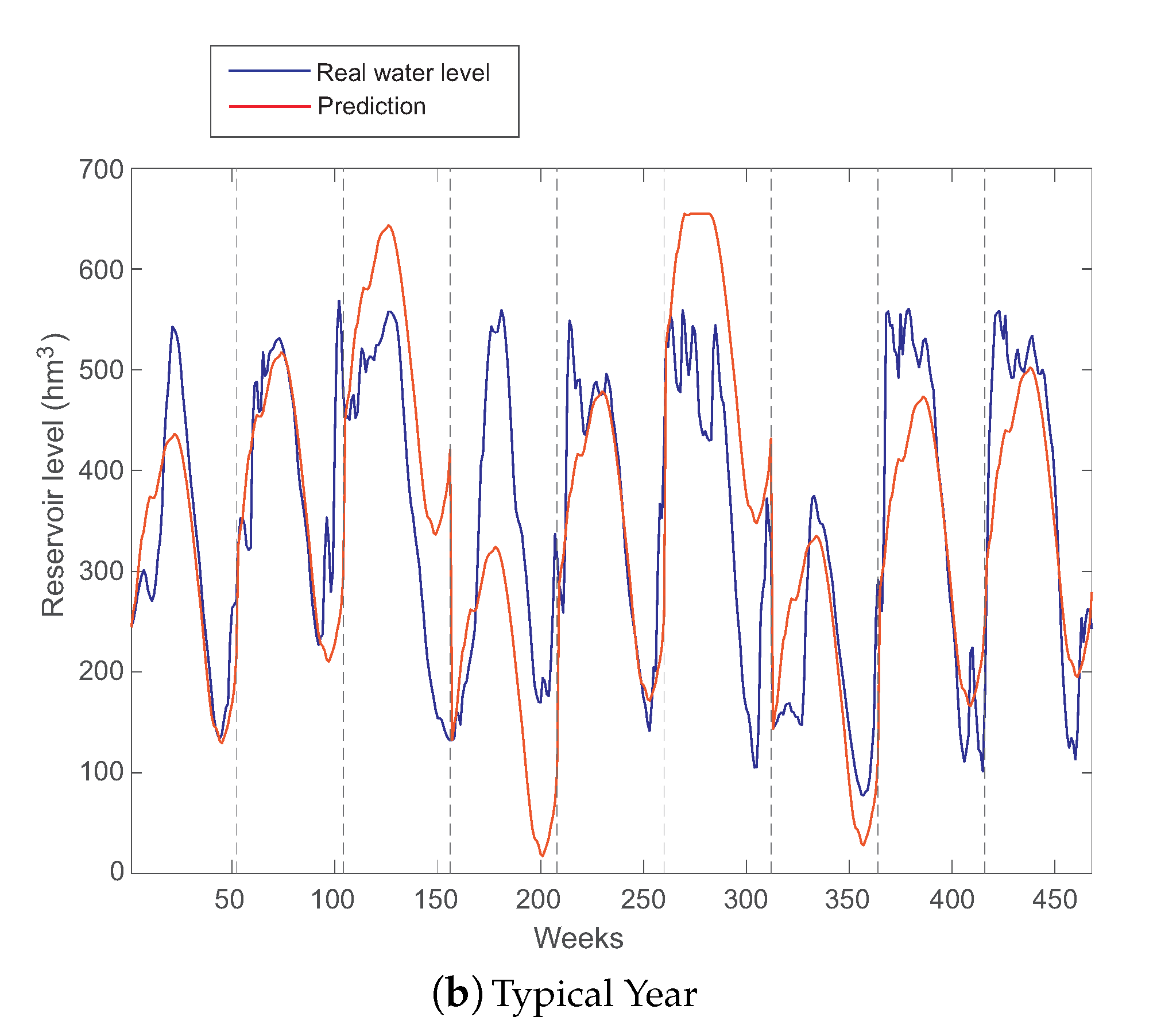
2.4. Typical Year Prediction Approach

The typical year prediction approach is one of the most frequently used persistence-based approach among the last decades. It is a statistical model which assumes processes repeat over time, specifically with a period of one year. The time step can be any period of time less than a year, such as hours, days, or months, but in the present study we used weeks.

Focusing on our purpose, let us consider a training set $\left\{x_i\left(t\right)\right|0<i\le T,0<t\le N\}$ of dammed water level time series of the reservoir along T years. Each $x_i\left(t\right)$ stands for the dammed water level at the ith year during the week t. The number of weeks per year are fixed to $N=52$. From this training set, the corresponding vector of residuals $r_i\left(t\right)$ are created, defined as $r_i\left(t\right)=x_i(t+1)-x_i\left(t\right)$. Moreover, a matrix of residuals for all the training set is calculated:

$$M={\left(\begin{array}{ccccc}{r}_1\left(1\right)& \cdots & r_1\left(t\right)& \cdots & r_1\left(N\right)\\ ⋮& \ddots & \cdots & \ddots & ⋮\\ r_i\left(1\right)& \cdots & r_i\left(t\right)& \cdots & r_i\left(N\right)\\ ⋮& \ddots & \cdots & \ddots & ⋮\\ r_T\left(1\right)& \cdots & r_T\left(t\right)& \cdots & r_T\left(N\right)\end{array}\right)}_{T\times N},$$

(8)

where each coefficient $r_i\left(t\right)$,

$$r_i\left(t\right)=x_i(t+1)-x_i\left(t\right),1<t<N,1<i\le T,$$

(9)

stands for the residuals of the dammed water level in the reservoir in the week t of the ith year of the training set. The typical year prediction approach is then obtained by averaging the residuals over all years in the training set:

$$\overline{r}\left(t\right)=\frac{1}{T}\sum _{i=1}^T{r}_i\left(t\right),0<t<N.$$

(10)

Note that the average residual $\overline{r}\left(t\right)$ can be used to estimate the dammed water level as a typical year, just by setting the first measurement of the dammed water level in a given year in a test set:

$$\widehat{x}\left(t\right)=\left\{\begin{array}{cc}x\left(1\right),\hfill & t=1,\hfill \\ \widehat{x}(t-1)+\overline{r}(t-1),\hfill & 1<t\le N,\hfill \end{array}\right.$$

(11)

where $\widehat{x}\left(t\right)$ stands for the reservoir water level predicted for the week t.

2.5. Machine Learning Regression Techniques

Several ML regression algorithms were considered in this research, for the short-term dammed water level prediction at Belesar: Support Vector Regression (SVR) [35,36], Multi-layer Perceptron (MLP) [37,38], Extreme Learning Machine (ELM) [39,40], and Gaussian Process Regression (GPR) [41,42]. We outline some general characteristics of the applied methods. For instance, the ELM is a very fast-training algorithm, since it is based on a pseudo-inverse calculation. In contrast, the GPR is usually the most computationally-demanding model to be trained, and it has sometimes shown problems related to the amount of time required to train the model in large databases. On the other hand, although the MLP trained with the backpropagation algorithm [43] with stochastic gradient descent [44] is a strong regression approach, it is computationally more demanding than the ELM since it has to iterate the data multiple times to adjust the weights of the model. Finally, the SVR computational burden is comparable to the MLP.

The implementations of the proposed ML regression techniques are those supported by the R language in the cases of ELM and SVR, where the libraries used are: elmNNRcpp [45] for ELM; e1071 [46] for the implementation of the SVR algorithm; and the Python library scikit-learn MLP and GPR [47,48].

2.5.1. Support Vector Regression

SVR [35] is a well-established algorithm for regression and function approximation problems. SVR takes into account an error approximation to the data, as well as the ability to improve the prediction of the model when a new dataset is evaluated. Although there are several versions of the SVR algorithm, we used the classical model ($ϵ$-SVR) described in detail in [35], which has been used for many problems and applications in science and engineering [36].

The $ϵ$-SVR method for regression starts from a given set of training vectors ${\left\{({\mathbf{x}}_i,{\vartheta }_i)\right\}}_{i=1}^N$ and models the input–output relation as the following general model:

$$\widehat{\vartheta }\left(\mathbf{x}\right)=g\left(\mathbf{x}\right)+b={\mathbf{w}}^T\varphi \left(\mathbf{x}\right)+b,$$

(12)

where ${\mathbf{x}}_i$ represents the input vector of predictive variables and ${\vartheta }_i$ stands for the value of the objective variable $\vartheta$ corresponding to the input vector ${\mathbf{x}}_{\mathbf{i}}$, the water level in the reservoir in this case. $\widehat{\vartheta }\left(\mathbf{x}\right)$ represents the model which estimates $\vartheta \left(\mathbf{x}\right)$. The parameters $(\mathbf{w},b)$ are determined to match the training pair set, where the bias parameter b appears separated here. The function $\varphi \left(\mathbf{x}\right)$ projects the input space onto the feature space. During the training, algorithms seek those parameters of the model which minimize the following risk function:

$$R\left[\widehat{\vartheta }\right]=\frac{1}{2}{∥\mathbf{w}∥}^2+C\sum _{i=1}^{N}L\left({\vartheta }_i,\widehat{\vartheta }\left({\mathbf{x}}_i\right)\right),$$

(13)

where the norm of $\mathbf{w}$ controls the smoothness of the model and $L\left({\vartheta }_i,\widehat{\vartheta }\left({\mathbf{x}}_i\right)\right)$ stands for the selected loss function. We used the $L^1$-norm modified for SVR and characterized by the $ϵ$-insensitive loss function [35]:

$$dL\left({\vartheta }_i,g\left({\mathbf{x}}_i\right)\right)=\left\{\begin{array}{cc}0\hfill & \mathrm{if}|{\vartheta }_i-g\left({\mathbf{x}}_i\right)|\le ϵ\hfill \\ |{\vartheta }_i-g\left({\mathbf{x}}_i\right)|-ϵ\hfill & \mathrm{otherwise}.\hfill \end{array}\right.$$

(14)

Figure 3 shows an example of the process of a SVR for a two-dimensional regression problem, with an $ϵ$-insensitive loss function.

To train this model, it is necessary to solve the following optimization problem [35]:

$$\begin{array}{cc}\hfill \underset{\mathbf{w},b,\xi }{min}& \frac{1}{2}\parallel \mathbf{w}\parallel +C\sum _{i=1}^N{\xi }_i+{\xi }_i^{*},\hfill \\ \hfill \mathrm{s}.\mathrm{t}.& {\vartheta }^i-{\mathbf{w}}^T\varphi \left({\mathbf{x}}_i\right)-b\le ϵ+{\xi }_i,\hfill & \hfill i=1,\dots ,N,\\ \hfill & -{\vartheta }^i+{\mathbf{w}}^T\varphi \left({\mathbf{x}}_i\right)+b\le ϵ+{\xi }_i^{*},\hfill & \hfill i=1,\dots ,N,\\ \hfill & {\xi }_i,{\xi }_i^{*}\ge 0,\hfill & \hfill i=1,\dots ,N.\end{array}$$

(15)

The dual form of this optimization problem is obtained through the minimization of a Lagrange function, which is constructed from the objective function and the problem constraints:

$$\begin{array}{ccc}\hfill \underset{\alpha ,{\alpha }^{*}}{max}-\frac{1}{2}\sum _{i,j=1}^N({\alpha }_i-{\alpha }_i^{*})& ({\alpha }_j-{\alpha }_j^{*})K({\mathbf{x}}_i,{\mathbf{x}}_j)-\hfill & ϵ\sum _{i=1}^N({\alpha }_i+{\alpha }_i^{*})+\sum _{i=1}^N{\vartheta }^i({\alpha }_i-{\alpha }_i^{*}),\hfill \\ \hfill \mathrm{s}.\mathrm{t}.& \sum _{i=1}^l({\alpha }_i-{\alpha }_i^{*})=0,\hfill & i=1,\dots ,N,\hfill \\ \hfill & {\alpha }_i,{\alpha }_i^{*}\ge 0,\hfill & i=1,\dots ,N,\hfill \\ \hfill & -{\alpha }_i,-{\alpha }_i^{*}\ge -C,\hfill & i=1,\dots ,N.\hfill \end{array}$$

(16)

In the dual formulation of the problem, the function $K({\mathbf{x}}_i,{\mathbf{x}}_j)$ represents the inner product $〈\varphi \left({\mathbf{x}}_i\right),\varphi \left({\mathbf{x}}_j\right)〉$ in the feature space. Any function $K({\mathbf{x}}_i,{\mathbf{x}}_j)$ may become a kernel function as long as it satisfies the constraints of the inner products. It is very common to use the Gaussian radial basis function:

$$K({\mathbf{x}}_i,{\mathbf{x}}_j)=exp(-\gamma ·{∥{\mathbf{x}}_i-{\mathbf{x}}_j∥}^2).$$

(17)

The final form of the function $g\left(\mathbf{x}\right)$ depends on the Lagrange multipliers ${\alpha }_i,{\alpha }_i^{*}$ as:

$$g\left(\mathbf{x}\right)=\sum _{i=1}^N({\alpha }_i-{\alpha }_i^{*})K({\mathbf{x}}_i,\mathbf{x}).$$

(18)

Incorporating the bias, the estimation of the dammed water level in the reservoir is finally made by the following expression:

$$\widehat{\vartheta }\left(\mathbf{x}\right)=g\left(\mathbf{x}\right)+b=\sum _{i=1}^N({\alpha }_i-{\alpha }_i^{*})K({\mathbf{x}}_i,\mathbf{x})+b.$$

(19)

2.5.2. Multi-Layer Perceptrons

A multi-layer perceptron is a particular class of Artificial Neural Network (ANN), which has been successfully applied to solve a large variety of non-linear problems, mainly classification and regression tasks [37,38]. The multi-layer perceptron consists of an input layer, a number of hidden layers, and an output layer, all of which are basically composed by a number of special processing units called neurons. All neurons in the network are connected to other neurons by means of weighted links (see Figure 4). In the feedforward multi-layer perceptron, the neurons within a given layer are connected to those of the previous layers. The values of these weights are related to the ability of the multi-layer perceptron to learn the problem, and they are learned from a sufficiently long number of examples. The process of assigning values to these weights from labeled examples is known as the training process of the perceptron. The adequate values of the weights minimizes the error between the output given by the multi-layer perceptron and the corresponding expected output in the training set. The number of neurons in the hidden layer is also a parameter to be optimized [37,38].

The input data for the multi-layer perceptron consist of a number of samples arranged as input vectors ${\{{\mathbf{x}}^i\in {\mathbb{R}}^n\}}_{i=1}^N$, where each input vector ${\mathbf{x}}^i=(x_1^i,\cdots ,x_n^i)$. Once a multi-layer perceptron has been properly trained, validated, and tested using an input vector different from those contained in the database, it is able to generate an estimated output $\vartheta \in \mathbb{R}$. The relationship between the output $\vartheta$ and a generic input signal $\mathbf{x}=(x_1,\cdots ,x_n)$ of a neuron is:

$$\vartheta \left(\mathbf{x}\right)=\phi \left(\sum _{j=1}^n{w}_j{x}_j-b\right),$$

(20)

where $\vartheta$ is the output signal, $x_j$ for $j=1,\dots ,n$ are the input signals, $w_j$ is the weight associated with the jth input, and b is the bias term [37,38]. The transfer function $\phi$ is usually considered as the logistic function:

$$\phi \left(x\right)=\frac{1}{1+e^{-x}}.$$

(21)

The well-known Stochastic Gradient Descent (SGD) algorithm is often applied to train the multi-layer perceptron [44]. In this case, we use the scikit-learn implementation of the multi-layer perceptron with the SGD training algorithm.

2.5.3. Extreme-Learning Machines

The extreme-learning machine [39] is a fast training method for neural networks, which can be applied to feed-forward perceptron structures (see Figure 4). In ELM, the network weights of the first layer are randomly set, after which a pseudo-inverse of the hidden-layer output matrix is obtained. This pseudo-inverse is then used to obtain the weights of the output layer which best fit the objective values. The advantage of this method is not only that it is extremely fast, but also that it obtains competitive results versus other established approaches, such as classical training for multi-layer perceptrons, or even SVM algorithms. The universal-approximation capability of the ELM is proven in [40].

The ELM algorithm can be summarized by considering a training set $\left\{({\mathbf{x}}_i,{\vartheta }_i)\right|{\mathbf{x}}_i\in {\mathbb{R}}^n,{\vartheta }_i\in \mathbb{R},1\le i\le N\}$, an activation function $g\left(x\right)$, and a given number of hidden nodes $\tilde{N}$, and applying the following steps:

1.

Randomly assign input weights ${\mathbf{w}}_i$ and the bias $b_i$, where $i=1,\dots ,\tilde{N}$, using a uniform probability distribution in $[-1,1]$.

2.

Calculate the hidden-layer output matrix $\mathbf{H}$, defined as follows:

$$\mathbf{H}={\left[\begin{array}{ccc}g({\mathbf{w}}_1{\mathbf{x}}_1+b_1)& \cdots & g({\mathbf{w}}_{\tilde{N}}{\mathbf{x}}_1+b_{\tilde{N}})\\ ⋮& \cdots & ⋮\\ g({\mathbf{w}}_1{\mathbf{x}}_N+b_1)& \cdots & g({\mathbf{w}}_{\tilde{N}}{\mathbf{x}}_N+b_{\tilde{N}})\end{array}\right]}_{N\times \tilde{N}}.$$

(22)

3.

Calculate the output weight vector $\beta$ as follows:

$$\beta ={\mathbf{H}}^{†}\mathbf{T},$$

(23)

where ${\mathbf{H}}^{†}$ is the Moore–Penrose inverse of the matrix $\mathbf{H}$ [39] and $\mathbf{T}$ is the training output vector, $\mathbf{T}={[{\vartheta }_1,\dots ,{\vartheta }_N]}^T$.

Note that the number of hidden nodes $\tilde{N}$ is a free parameter to be set before the training of the ELM algorithm, and it must be estimated for obtaining good results by scanning a range of $\tilde{N}$. In this study, we used the ELM implemented in Matlab by G. B. Huang, freely available at [45].

2.5.4. Gaussian Processes for Regression

A Gaussian Process for Regression (GPR) is a supervised-learning method designed for solving regression problems. In this section, we give a short description of the most important characteristics of the GPR algorithm. The interested reader can consult exhaustive reviews for further information [41,42].

Given a set of n-dimensional inputs ${\mathbf{x}}_i\in {\mathbb{R}}^n$ and their corresponding scalar outputs ${\vartheta }_i\in \mathbb{R}$, for the dataset ${\mathcal{D}}_S\equiv {\left\{({\mathbf{x}}_i,{\vartheta }_i)\right\}}_{i=1}^N$, the regression task obtains the predictive distribution for the corresponding observation ${\vartheta }_{*}$ based on ${\mathcal{D}}_S$, given a new input ${\mathbf{x}}_{*}$.

The GPR model assumes that the observations can be modeled as some noiseless latent function of the inputs, in addition to an independent noise, $\vartheta =f\left(\mathbf{x}\right)+\epsilon$, and then specifies a zero-mean Gaussian process for both the latent function $f\left(\mathbf{x}\right)$$\sim \mathcal{GP}$$(0,k(\mathbf{x},{\mathbf{x}}^{\prime }))$ and the noise $\epsilon \sim \mathcal{N}(0,{\sigma }^2)$, where $k(\mathbf{x},{\mathbf{x}}^{\prime })$ is a covariance function and ${\sigma }^2$ is a hyper-parameter that specifies the error variance.

The covariance function $k(\mathbf{x},{\mathbf{x}}^{\prime })$ specifies the degree of coupling between $\vartheta \left(\mathbf{x}\right)$ and $\vartheta \left({\mathbf{x}}^{\prime }\right)$ and encodes the properties of the Gaussian process, such as the variance and smoothness. One of the most used covariance functions is the anisotropic-squared exponential, which has the form of an unnormalized Gaussian function, $k(\mathbf{x},{\mathbf{x}}^{\prime })={\sigma }_0^{2}exp\left(-\frac{1}{2}{\mathbf{x}}^T{{\Lambda }}^{-1}\mathbf{x}\right)$, and depends on the signal power ${\sigma }_o^2$ and length scales ${\Lambda }$, where ${\Lambda }$ is a diagonal matrix containing one length scale per input dimension. Each length scale controls the degree to which the correlation between outputs decay as the separation along the corresponding input dimension grows. We collectively refer to all kernel parameters as $\theta$.

The joint distribution of the available observations (collected in $\vartheta$) and some unknown output $\vartheta \left({\mathbf{x}}_{*}\right)$ form a multivariate Gaussian distribution, the parameters of which are specified by the covariance function:

$$\left[\begin{array}{c}\vartheta \\ {\vartheta }_{*}\end{array}\right]\sim \mathcal{N}\left(0,\left[\begin{array}{cc}\mathbf{K}+{\sigma }^2{\mathbf{I}}_N& {\mathbf{k}}_{*}\\ {\mathbf{k}}_{*}^T& k_{**}+{\sigma }^2\end{array}\right]\right),$$

(24)

where ${\left[\mathbf{K}\right]}_{n{n}^{\prime }}=k({\mathbf{x}}_n,{\mathbf{x}}_{n^{\prime }})$, ${\left[{\mathbf{k}}_{*}\right]}_n=k({\mathbf{x}}_n,{\mathbf{x}}_{?})$, and $k_{**}=k({\mathbf{x}}_{*},{\mathbf{x}}_{*})$. Here, ${\mathbf{I}}_N$ is used to denote the identity matrix of size N. The notation ${\left[\mathbf{A}\right]}_{n{n}^{\prime }}$ refers to the entry at row n, column $n^{\prime }$ of $\mathbf{A}$. Likewise, ${\left[\mathbf{a}\right]}_n$ is used to reference the nth element of vector $\mathbf{a}$.

From Equation (24) and the conditioning on the observed training outputs, we obtain the predictive distribution as:

$$\begin{array}{c}{p}_{GP}\left({\vartheta }_{*}\right|{\mathbf{x}}_{*},\mathcal{D})=\mathcal{N}\left({\vartheta }_{*}\right|{\mu }_{GP*},{\sigma }_{GP*}^2)\hfill \\ {\mu }_{GP*}={\mathbf{k}}_{*}^T{(\mathbf{K}+{\sigma }^2{\mathbf{I}}_N)}^{-1}\vartheta \hfill \\ {\sigma }_{GP*}^2={\sigma }^2+k_{**}-{\mathbf{k}}_{*}^T{(\mathbf{K}+{\sigma }^2{\mathbf{I}}_N)}^{-1}{\mathbf{k}}_{*},\hfill \end{array}$$

(25)

which is computed $\mathcal{O}\left(N^3\right)$ times, due to the inversion of the $N\times N$ matrix $\mathbf{K}+{\sigma }^2{\mathbf{I}}_N$.

The hyper-parameters $\{\theta ,\sigma \}$ are typically selected by maximizing the marginal likelihood of the observations, which is

$$\begin{array}{c}logp\left(\vartheta \right|\theta ,\sigma )=-\frac{1}{2}{\mathbf{y}}^T{(\mathbf{K}+{\sigma }^2{\mathbf{I}}_N)}^{-1}\vartheta -\hfill \\ \hfill -\frac{1}{2}|\mathbf{K}+{\sigma }^2{\mathbf{I}}_N|-\frac{N}{2}log\left(2\pi \right).\end{array}$$

(26)

Observe that, by providing analytical derivatives of Equation (26), gradient methods reduce their computation time to an order $\mathcal{O}\left(N^3\right)$.

3. Experiments and Results

We experimentally evaluated the different long- and short-term approaches used for the analysis of Belesar reservoir water level. First, we detail the experimental design carried out both for long- and short-term analyses of the dammed water level. We also describe the error metric used in the short-term analysis of water level in the reservoir. The experimental results for the long-term case are shown after, together with a discussion based on DFA, ARMA, and typical year persistence-based results. This experimental evaluation is closed with the short-term results of dammed water level, focused on a weekly time-horizon prediction problem, and how ML algorithms perform on this problem.

3.1. Experimental Design

The methodology used in this study is introduced in Section 2, but it is explained here in more detail. The long-term analysis was carried out through the DFA on the dammed water level times series, since 1963. This analysis shows that persistence-based approaches, such as ARMA and persistence-based models, are a good option to obtain long-term predictions for the water level at this reservoir. In the short-term case, we considered exogenous variables, and analysis from 2009 to 2015. In this case, for all the datasets considered (see Table 2), two types of experiments were carried out. The first one considered all the weeks in the training set ordered sequentially, whereas in the second one we carried out a seasonal analysis for all the available years (2009–2015). In the first experimental design, two hold-out schemes were used for partitioning the data into a training and test set: a random or shuffle partition and a “temporal” partition. In the shuffle split, each week was chosen randomly to belong to either training or test set, with a proportion of $80\%$ of the data in the training set and the remaining $20\%$ used to test the performance of the model. In the temporal split, the first $80\%$ of the weeks, ordered sequentially, were used for training purposes, and the rest for testing the model. In the second experimental design, the one with a table for each season, only the temporal split was considered.

For the three resulting data partitions, the four regression techniques summarized in Section 2.5 were applied. Other hyper-parameters associated with each method were tuned using an internal k-fold cross-validation ($k=3$) over the training data. The parameter values were explored using a grid-search, in such a way that every classifier was run $3\times C$ times, where C is the number of all possible parameter combinations. The combination of parameters leading to the lowest average validation $RMSE$ from this three-fold cross-validation was selected as the optimal one, and the training process was finally repeated using this configuration. The values explored for each hyper-parameter in the ML techniques are shown in

Table 3. Configuration parameters of the ML regressors considered.

MLP
Transfer function: {Logistic, Hyperbolic Tangent, ReLU}
Architecture: {25, 50, 75, 100, 125, 25:25, 50:50, 75:75,
50:50:50, 75:50:25}
${\mathit{L}}_{\mathbf{2}}$: $0.0035$
Learning rate: {$0.0001$, $0.00085$, $0.0016$,
$0.00235$, $0.0031$, $0.00385$, $0.0046$}
Training algorithms:
{Stochastic Gradient Descent: $\mu$ = {$0.9$, $0.85$, $0.7$},
Adam: ${\beta }_1$ = $0.9$, ${\beta }_2$ = $0.999$ }
SVR Linear
C: $\{0.25,0.5,1,2,4,...,512\}$
$ϵ:$$\{0,0.25,...,0.2\}$
SVR rbf
C: $\{0.25,0.5,1,2,4,...,512\}$
$ϵ:$$\{0,0.25,...,0.2\}$
$\gamma :$$\{\frac{1}{N},\frac{1}{N}+0.1,...,0.4\}$,
(where N is the number of input variables)
GPR
Kernel: {Dot Product, Radial,
Dot Product + White Noise}
$\alpha :$$1\times {10}^{-6}$
ELM
Transfer function: {ReLU, Sigmoid, Radial}
Number of layers: 1
Number of neurons: {50, 75}

, where the values included in curly brackets are the ranges used in the search process, and those that are not in brackets are fixed for all combinations. In the case of the architecture of the MLP, the values shown are the number of neurons in each layer (separated by a colon; the architectures explored range from one to three layers). In the tables where the experimental results are shown (

Table 4. Results of the different ML regression techniques for different variables considered (datasets) in the case of standard data (all seasons) and random partitioning. Boldface stands for the best value found in a dataset, and italic for the second best.

Dataset	Model	RMSE (hm${}^3$)	MAE (hm${}^3$)
1	ELM	33.68	19.61
1	SVM (lin)	35.85	22.76
1	SVM (rbf)	24.63	16.37
1	MLP	24.86	16.45
1	GPR	32.51	21.10
2	ELM	33.17	20.22
2	SVM (lin)	30.52	18.49
2	SVM (rbf)	30.63	22.42
2	MLP	22.94	16.28
2	GPR	36.91	21.57
3	ELM	32.50	17.93
3	SVM (lin)	28.72	15.58
3	SVM (rbf)	30.35	20.80
3	MLP	20.20	14.26
3	GPR	34.27	18.12
4	ELM	31.13	17.99
4	SVM (lin)	27.65	15.04
4	SVM (rbf)	29.79	20.24
4	MLP	20.44	14.04
4	GPR	36.22	18.29

and

Table 5. Results of the different ML regression techniques for different variables considered (datasets) in the case of standard data (all seasons) and temporal partitioning. Boldface stands for the best value found in a dataset, and italic for the second best.

Dataset	Model	RMSE (hm${}^3$)	MAE (hm${}^3$)
1	ELM	24.27	17.48
1	SVM (lin)	19.96	16.18
1	SVM (rbf)	19.34	14.55
1	MLP	21.66	17.24
1	GPR	21.74	18.28
2	ELM	24.86	18.31
2	SVM (lin)	25.35	20.79
2	SVM (rbf)	22.56	16.46
2	MLP	23.42	17.38
2	GPR	24.43	19.28
3	ELM	21.59	14.56
3	SVM (lin)	16.44	11.28
3	SVM (rbf)	19.28	12.09
3	MLP	21.12	15.17
3	GPR	17.00	11.99
4	ELM	22.87	15.10
4	SVM (lin)	18.60	12.74
4	SVM (rbf)	21.88	14.25
4	MLP	20.37	15.19
4	GPR	18.65	13.40

), only the best configuration for each model is included. Note that, for MLP, the best configuration was consistently the one with one layer and 100 neurons, using a hyperbolic tangent as transfer function. In addition, for the GPR, the best kernel was always the dot product. For ELM, the best results were always obtained with a sigmoid function and 50 hidden neurons. Finally, it is important to outline that the test set was never used during parameter tuning.

Note that, for the methods that have a stochastic nature (caused by the training algorithm or the weight initialization), as in the case of MLP, ELM, or GPR, all experiments were run 30 times and the mean value was obtained. For MLP, which involves an iterative training, a stopping criterion was used to prevent overfitting. This caused the training to stop when the validation score stopped improving by less than ${10}^{-4}$ for 10 consecutive iterations. In GPR, a cross-validation method during the maximization of the marginal likelihood was done to prevent the overfitting. Note the obtained results over the test data partition suggest that the evaluated ML methods did not overfit.

Regarding the evaluation metrics for short-term analysis, we considered two metrics for comparison purposes: the Root Mean Square Error (RMSE) and the Mean Absolute Error (MAE). RMSE calculates the value of the root square of the squared difference between the ground truth, ${\vartheta }_i$, and the predicted value, ${\widehat{\vartheta }}_i$, and gives an average for all examples predicted:

$$RMSE=\frac{1}{N}\sqrt{\sum _{i=1}^N{({\vartheta }_i-{\widehat{\vartheta }}_i)}^2},$$

(27)

MAE calculates the value of the difference between the ground truth, ${\vartheta }_i$, and the predicted value, $\widehat{{\vartheta }_i}$, in absolute value, and gives an average for all examples predicted:

$$MAE=\frac{1}{N}\sum _i^N|{\vartheta }_i-{\widehat{\vartheta }}_i|.$$

(28)

Both errors are measured in the same units as the variable under study (in our case, hm${}^3$) and have been widely used for model evaluation [25,26,27,28,29]. While MAE gives the same weight to all errors, RMSE penalizes variance as it gives errors with larger absolute values more weight than errors with smaller absolute values. Both aspects are important and should be taken into account during the model evaluation.

3.2. Long-Term Reservoir Level Analysis

We first applied the DFA algorithm to the complete time series of dammed water level at Belesar. Figure 5 shows the DFA obtained. As can be seen, there is a clear two-ranges structure with separation point at around 52 weeks, which matches a year duration. Up to 52 weeks, the dammed water level time series is extremely long-term correlated, as the correlation exponent $\alpha \approx 1.52$ (recall that an exponent $\alpha =0.5$ represents an uncorrelated process). Over 52 weeks, the time series is mostly uncorrelated since the correlation exponent is $\alpha \approx 0.57$, very close to $0.5$. This result suggests a process with a strong annual period. This justifies the use of persistence-based techniques for analysis of the time series, such as the typical year approach or auto-regressive methods, as good options to obtain accurate long-term predictions of the weekly dammed water level at Belesar.

We therefore evaluated the application of ARMA and typical year persistence-based models for this long-term analysis of water level in Belesar reservoir. We varied the ARMA parameters p and q from 0 to 12 to determine the optimum ARMA model. Finally, the ARMA(9,0) = AR(9) obtained the best results.

Figure 6a,b shows the performance of an AR(9) model (the best auto-regressive method obtained) and the typical year method for dammed water level prediction respectively. Note that, in both cases, we used as training set the values of the dammed water level time series from 1963 to 2006. The model parameters were estimated in the training set, and the results are reported in the test set. As can be seen, the AR(9) model fits most of the dammed water level series. In general, the AR model is able to estimate the trend of the dammed water level time series, obtaining a reasonable result.

The fact that an AR model obtains good results in the prediction indicates that the prediction approach via typical year should also work fine in the prediction of water level at Belesar. This is also expected after the DFA analysis carried out at the beginning of this discussion. Figure 6b shows the performance of the typical year persistence-based method in the test set of Belesar. As can be seen, this approach is very effective in different years, which perfectly fit the typical year. There are, however, other years in which the typical year prediction does not work as well, which indicates that those years present anomalies in terms of the dammed water level, which may be associated with rainfall anomalies, droughts, etc. In general, the prediction given by the typical year is smoother than that of the best AR model found, which seems to indicate that the water level at Belesar has a very important intra-annual persistence, and a small inter-annual contribution, as shown in the DFA analysis of the dammed water level time series.

3.3. Short-Term Reservoir Level Prediction

In this section, we evaluate the performance of different ML regressors in a short-term (one week time-horizon) dammed water level prediction problem at Belesar reservoir. We structured the experiments carried out by the type of data considered (standard, i.e., all seasons, or seasonal) and by the type of train-test partitioning: random or temporal partitioning.

3.3.1. Standard Data, Random Partitioning

Figure 7 shows the results obtained in this experiment considering standard data and random partition for test. Table 4 presents the detailed numerical results of the experiment.

The best model in these set of experiments was an MLP with the input variables defined in Dataset 3 (see Table 2). Figure 8 shows the best prediction obtained by MLP in the test set, plotted against the ground truth. As can be seen, the prediction obtained by MLP is excellent, being close to the dammed water level ground truth. Note that, since random data were considered, there is no time relation between each of the samples shown, which does not allow checking how the regressor model manages the temporal character of the time series. However, observe that both RMSE and MAE values are extremely good, which indicates that MLP is able to obtain an extremely accurate weekly prediction of water level in reservoir based on the variables specified in Dataset 3.

3.3.2. Standard Data, Temporal Partitioning

In the experiment where the standard data and a temporal split partition were used, the best results obtained in the different datasets considered are depicted in Figure 9 and numerically detailed in Table 5.

In this case, the best model is the SVR with linear kernel in Dataset 3.

Figure 10 shows the prediction obtained with SVR together with the ground truth for each test sample. As can be seen, in this case the data shape is smoother, given the continuity in time of the data samples. This allows checking the temporal behavior of the prediction algorithm, given that the model is fed $({\mathbf{X}}_t,y_t)$ to predict $y_{t+1}$, which could not be observed in the previous experiment. It seems that the temporal continuity in the data has helped the model make a better prediction, as can be seen in the improvement of the results in both error metrics considered. The SVR result fits extremely well to the ground truth, having a few small abrupt errors in some areas where there are notable changes. Note that the SVR has correctly accounted for this intrinsic characteristic of the data and with great success.

3.3.3. Seasonal Data, Temporal Partitioning

Finally, we considered an experiment with seasonal data and temporal partitioning. We skipped the experiment with random partitioning since the ML algorithms obtain worse results here. The results obtained in this case of seasonal data and a temporal partition are shown in

Table 6. Best results obtained for the case of temporal partitioning. Only the best algorithm in each season and dataset are detailed in this table.

Season	Model	Dataset	RMSE (hm${}^3$)	MAE (hm${}^3$)
Spring	SVR (Linear)	3	17.41	13.94
Summer	ELM	1	7.83	5.73
Autumn	Gaussian Process	3	14.40	11.01
Winter	SVR (RBF)	1	22.14	15.39
	Average Metrics		15.45	11.52

.

The results in Table 6 can be better interpreted if they are observed along with the predictions shown in Figure 11. It is easy to see that the most difficult season to predict seems to be winter, where the SVR (best model) uses the bare minimum information, only the upstream and tributaries’ flows. Note, however, that the same behavior is observed in summer, which is apparently the simplest season to predict (it seems to be quite linear with negative slope). In this case, it is the ELM regressor that provides the best result, also using Dataset 1 (upstream and tributaries’ flows). The complexity in winter seems to be well modeled by the SVR with RBF. In spring, the data seem fairly similar to summer, and they are modeled with a simple model, a linear SVR. In this case, it uses a higher number of variables (Dataset 3) to predict the apparent changes in trend of the data, which seem to first decrease, then increase, and slightly start to decrease again. The autumn data have more complexity, but they are modeled correctly with a GPR and a higher number of variables (Dataset 3).

3.3.4. Discussion on Short-Term Prediction Results

Table 7. General comparison of the experimental results in the short-term prediction of water level at Belesar reservoir. Boldface stands for the best value found in a dataset, and italic for the second best.

Experiment	RMSE (hm${}^3$)	MAE (hm${}^3$)
Standard data, random partitioning	20.20	14.26
Standard data, temporal partitioning	16.44	11.28
Seasonal data, temporal partitioning	15.45	11.52

shows the results obtained in each experiment carried out for the short-term prediction of dammed water level at Belesar reservoir. Note that the best overall result according to RMSE was obtained with the configuration seasonal data, temporal partition, which uses four different ML models for each season. According to MAE, the best overall result was obtained with the configuration standard data, temporal partitioning using a SVR algorithm.

Some specific remarks can be given when the results in Table 4 and Table 5 are analyzed in detail. Note that including the snow variable in the predictive variables (Dataset 4) worsens the results obtained with the variables in Dataset 3. This seems to indicate that snow is not a key variable for this specific reservoir, even though it is known to be important at other locations. We can also observe that, in general, the most relevant variable to predict the dammed water level in the reservoir is the upstream and tributaries’ flow, and not the precipitation amount or the output of the dam for electricity production.

4. Conclusions

In this study, we carried out a complete investigation on the long- and short-term prediction of dammed water level for hydropower generation at a reservoir in Miño River (Belesar, Spain). Different techniques were explored, such as Detrended Fluctuation Analysis, Auto-regressive models, persistence-based techniques, and Machine Learning (ML) regression algorithms.

The long-term analysis of the dammed water level showed a clear annual persistence of the signal, which allows applying auto-regressive and persistence-based algorithms with success for this problem. We showed that, depending on the year analyzed, persistence-based approaches such as a typical year are able to model the water level of the reservoir with a high accuracy.

In the short-term analysis, we tackled a prediction problem of the water level at the reservoir with a prediction time-horizon of one week, by using different ML regression techniques and exogenous hydro-meteorological variables. In this case, we showed that the ML algorithms are able to obtain extremely accurate results. We showed that the predictability of dammed water level of the reservoir is highly based on variables such as upstream and tributaries flow. On the contrary, the precipitation measurements and dam outputs for hydropower production proved to be less relevant variables to predict the dammed water level.

Note that this work is based on measurements and data from a single reservoir (Belesar, Galicia, Spain). This reservoir is interesting since it is mainly devoted to hydropower generation, but it is also used in part to cover human consumption. Measuring stations installed upstream Miño River and on its tributaries provide rich information about the amount of water poured into the reservoir. Thus, note that this reservoir has all the elements needed to explore the performance of both long- and short-term algorithms in a water level prediction problem. All the algorithms developed for this reservoir are directly applicable to any other site with similar rich information of measurements and data. Of course, specific hydro-meteorological characteristics of the zone will not be exportable to other specific areas with different hydro-meteorological characteristics. For example, we showed that snow is not a very important feature in the short-term water level prediction of this reservoir, even though it is known that it is in fact a key feature in other reservoirs, mainly in springtime [49]. However, note that the methodology reported here, both for long- and short-term prediction, is able to detect the importance of specific hydro-meteorological features at any other reservoir where it is applied.

Finally, this work opens new lines of research, e.g., testing alternative regression techniques such as random forest or grammatical evolution, among others, and exploring alternative exogenous atmospheric variables which can provide information to improve the water level prediction of the reservoir.

References

1. Zhang, D.; Lin, J.; Peng, Q.; Wang, D.; Yang, T.; Sorooshian, S.; Liu, X.; Zhuang, J. Modeling and simulating of reservoir operation using the artificial neural network, support vector regression, deep learning algorithm. J. Hydrol. 2018, 565, 720–736. [Google Scholar] [CrossRef] [Green Version]
2. Lehner, B.; Liermann, C.R.; Revenga, C.V.; Vörösmarty, C.; Fekete, B.; Crouzet, P. High-resolution mapping of the world’s reservoirs and dams for sustainable river-flow management. Front. Ecol. Enviorn. 2011, 9, 494–502. [Google Scholar] [CrossRef] [Green Version]
3. Akkose, A.; Bayraktar, A.; Dumanoglu, A.A. Reservoir water level effects on nonlinear dynamic response of arch dams. J. Fluids Struc. 2008, 24, 418–435. [Google Scholar] [CrossRef]
4. Wang, D.; Zhang, S.; Wang, G.; Han, Q.; Huang, G.; Wang, H.; Liu, Y.; Zhang, Y. Quantitative Assessment of the Influences of Three Gorges Dam on the Water Level of Poyang Lake, China. Water 2019, 11, 1519. [Google Scholar] [CrossRef] [Green Version]
5. Zhang, Y.; Zheng, H.; Herron, X.; Liu, X.; Wang, Z.; Chiew, F.W.; Parajka, J. A framework estimating cumulative impact of damming on downstream water availability. J. Hydrol. 2019, 575, 612–627. [Google Scholar] [CrossRef]
6. Chou, J.S.; Ho, C.C.; Hoang, H.S. Determining quality of water in reservoir using machine learning. Ecol. Inform. 2018, 44, 57–75. [Google Scholar] [CrossRef]
7. Ahmed, U.; Mumtaz, R.; Anwar, H.; Shah, A.A.; Irfan, R.; García-Nieto, J. Efficient water quality prediction using supervised Machine Learning. Water 2019, 11, 2210. [Google Scholar] [CrossRef] [Green Version]
8. Sentas, A.; Psilovikos, A. Comparison of ARIMA and Transfer Function (TF) Models in Water Temperature Simulation in Dam—Lake Thesaurus, Eastern Macedonia, Greece; Environmental Hydraulics—Christodoulou & Stamou, Ed.; CRC Press, Taylor and Francis Group: Boca Raton, FL, USA, 2010; Volume 2, pp. 929–934. [Google Scholar]
9. Xu, C.; Xu, Z.; Yang, Z. Reservoir operation optimization for balancing hydropower generation and biodiversity conservation in a downstream wetland. J. Clean. Prod. 2019, 118885. [Google Scholar] [CrossRef]
10. Jia, T.; Qin, H.; Yan, D.; Zhang, Z.; Liu, B.; Li, C. Short-Term Multi-Objective Optimal Operation of Reservoirs to Maximize the Benefits of Hydropower and Navigation. Water 2019, 11, 1272. [Google Scholar] [CrossRef] [Green Version]
11. Wei, C.C. Wavelet kernel support vector machines forecasting techniques: Case study on water-level predictions during typhoons. Expert Syst. Appl. 2012, 39, 5189–5199. [Google Scholar] [CrossRef]
12. Abdulkadir, T.S.; Salami, A.W.; Anwar, A.; Kareem, A.G. Modelling of hydropower reservoir variables for energy generation: Neural network approach. Ethiop. J. Enviorn. Stud. Manag. 2013, 6, 310–316. [Google Scholar] [CrossRef] [Green Version]
13. Ahmad, S.K.; Hossain, F. Maximizing energy production from hydropower dams using short-term weather forecasts. Ren. Energy 2020, 146, 1560–1577. [Google Scholar] [CrossRef]
14. Yadav, B.; Eliza, K. A hybrid wavelet-support vector machine model for prediction of Lake water level fluctuations using hydro-meteorological data. Measurement 2017, 103, 294–301. [Google Scholar] [CrossRef]
15. John, R.; John, M. Adaptation of the visibility graph algorithm for detecting time lag between rainfall and water level fluctuations in Lake Okeechobee. Adv. Water Res. 2019, 134, 103429. [Google Scholar] [CrossRef]
16. Zhang, Z.; Zhou, Y.; Liu, H.; Gao, H. In-situ water level measurement using NIR-imaging video camera. Flow Measur. Instrum. 2019, 67, 95–106. [Google Scholar] [CrossRef]
17. Vanthof, V.; Kelly, R. Water storage estimation in ungauged small reservoirs with the TanDEM-X DEM and multi-source satellite observations. Remote Sens. Environ. 2019, 235, 111437. [Google Scholar] [CrossRef]
18. Li, S.; Chen, J.; Xiang, J.; Pan, Y.; Huang, Z.; Wu, Y. Water level changes of Hulun Lake in Inner Mongolia derived from Jason satellite data. J. Vis. Commun. Image Rep. 2019, 58, 565–575. [Google Scholar] [CrossRef]
19. Plucinski, B.; Sun, Y.; Wang, S.Y.; Gillies, R.R.; Eklund, J.; Wang, C.C. Feasibility of Multi-Year Forecast for the Colorado River Water Supply: Time Series Modeling. Water 2019, 11, 2433. [Google Scholar] [CrossRef] [Green Version]
20. Pan, H.; Lv, X. Reconstruction of spatially continuous water levels in the Columbia River Estuary: The method of Empirical Orthogonal Function revisited. Est. Coast. Shelf Sci. 2019, 222, 81–90. [Google Scholar] [CrossRef]
21. Zhang, X.; Liu, P.; Zhao, Y.; Deng, C.; Li, Z.; Xiong, M. Error correction-based forecasting of reservoir water levels: Improving accuracy over multiple lead times. Environ. Model. Soft. 2018, 104, 27–39. [Google Scholar] [CrossRef]
22. Goovaerts, P. Geostatistical prediction of water lead levels in Flint, Michigan: A multivariate approach. Sci. Total Enviorn. 2019, 647, 1294–1304. [Google Scholar] [CrossRef] [PubMed]
23. Karri, R.R.; Wang, X.; Gerritsen, H. Ensemble based prediction of water levels and residual currents in Singapore regional waters for operational forecasting. Environ. Model. Soft. 2014, 54, 24–38. [Google Scholar] [CrossRef]
24. Bazartseren, B.; Hildebrandt, G. Short-term water level prediction using neural networks and neuro-fuzzy approach. Neurocomputing 2003, 55, 439–450. [Google Scholar] [CrossRef]
25. Chang, F.J.; Chang, Y.T. Adaptive neuro-fuzzy inference system for prediction of water level in reservoir. Adv. Water Res. 2006, 29, 1–10. [Google Scholar] [CrossRef]
26. Wang, A.P.; Liao, H.Y.; Chang, T.H. Adaptive Neuro-fuzzy Inference System on Downstream Water Level Forecasting. In Proceedings of the 2008 IEEE Fifth International Conference on Fuzzy Systems and Knowledge Discovery, Shandong, China, 18–20 October 2008; Volume 3, pp. 503–507. [Google Scholar] [CrossRef]
27. Yang, S.; Yang, D.; Chen, J.; Zhao, B. Real-time reservoir operation using recurrent neural networks and inflow forecast from a distributed hydrological model. J. Hydrol. 2019, 579, 124229. [Google Scholar] [CrossRef]
28. Chen, N.; Xiong, C.; Du, W.; Wang, C.; Lin, X.; Chen, Z. An Improved Genetic Algorithm Coupling a Back-Propagation Neural Network Model (IGA-BPNN) for Water-Level Predictions. Water 2019, 11, 1795. [Google Scholar]
29. Samadianfard, S.; Jarhan, S.; Salwana, E.; Mosavi, A.; Shamshirb, S.; Akib, S. Support Vector Regression Integrated with Fruit Fly Optimization Algorithm for River Flow Forecasting in Lake Urmia Basin. Water 2019, 11, 1934. [Google Scholar] [CrossRef] [Green Version]
30. Confederación Hidrográfica del Miño-Sil. Available online: https://www.chminosil.es/es/ (accessed on 23 March 2020).
31. Climate Data Store. Available online: https://cds.climate.copernicus.eu/cdsapp#!/search?type=dataset (accessed on 23 March 2020).
32. Yang, L.; Fu, Z. Process-dependent persistence in precipitation records. Phys. A 2019, 527, 121459. [Google Scholar] [CrossRef]
33. Dey, P.; Mujumdar, P.P. Multiscale evolution of persistence of rainfall and streamflow. Adv. Water Res. 2018, 121, 285–303. [Google Scholar] [CrossRef]
34. Box, G.P.; Jenkins, G.M.; Reinsel, G.C.; Ljung, G.M. Time Series Analysis: Forecasting and Control, 5th ed.; Wiley Series in Probability and Statistics; Wiley: Hoboken, NJ, USA, 2016. [Google Scholar]
35. Smola, A.J.; Schölkopf, B. A tutorial on support vector regression. Stat. Comput. 2004, 14, 199–222. [Google Scholar] [CrossRef] [Green Version]
36. Salcedo-Sanz, S.; Rojo, J.L.; Martínez-Ramón, M.; Camps-Valls, G. Support vector machines in engineering: An overview. WIREs Data Min. Know. Disc. 2014, 4, 234–267. [Google Scholar] [CrossRef]
37. Haykin, S. Neural Networks: A Comprenhensive Foundation; Prentice Hall: Upper Saddle River, NJ, USA, 1998. [Google Scholar]
38. Bishop, C.M. Neural Networks for Pattern Recognition; Oxford University Press: Oxford, UK, 1995. [Google Scholar]
39. Huang, G.B.; Zhu, Q.Y. Extreme learning machine: Theory and applications. Neurocomputing 2016, 70, 489–501. [Google Scholar] [CrossRef]
40. Huang, G.B.; Zhou, H.; Ding, X.; Zhang, R. Extreme Learning Machine for Regression and Multiclass Classification. IEEE Trans. Syst. Man Cyber. Part B 2012, 42, 513–529. [Google Scholar] [CrossRef] [PubMed] [Green Version]
41. Lázaro-Gredilla, M.; van Vaerenbergh, S.; NLawrence, N. Overlapping mixtures of gaussian processes for the data association problem. Patt. Recog. 2012, 45, 1386–1395. [Google Scholar] [CrossRef] [Green Version]
42. Rasmussen, C.E.; Williams, K.H. Gaussian Processes for Machine Learning; MIT Press: Cambridge, MA, USA, 2006. [Google Scholar]
43. Rumelhart, D.E.; Hinton, G.E.; Williams, R.J. Learning representations by back-propagating errors. Nature 1986, 323, 533–536. [Google Scholar] [CrossRef]
44. Amari, S. Backpropagation and stochastic gradient descent method. Neurocomputing 1993, 5, 185–196. [Google Scholar] [CrossRef]
45. Mouselimis, L.; Gosso, A. ELM R Code and Documentation. Available online: https://cran.r-project.org/package=elmNNRcpp (accessed on 23 March 2020).
46. Meyer, D.; Dimitriadou, E.; Hornik, K.; Weingessel, A.; Leisch, F.; Chang, C.; Lin, C. e1071 Package. Available online: https://cran.r-project.org/package=e1071 (accessed on 23 March 2020).
47. Pedregosa, F.; Varoquaux, G.; Gramfort, A.; Michel, V.; Thirion, B.; Grisel, O.; Blondel, M.; Blondel, M.; Weiss, R.; Dubourg, V.; et al. Scikit-Learn: Machine Learning in Python. J. Mach. Learn. Res. 2011, 12, 2825–2830. [Google Scholar]
48. Pedregosa, F.; Varoquaux, G.; Gramfort, A.; Michel, V.; Thirion, B.; Grisel, O.; Blondel, M.; Prettenhofer, P.; Weiss, R.; Dubourg, V.; et al. Scikit-Learn Library. Available online: https://scikit-learn.org/stable/ (accessed on 23 March 2020).
49. Denaro, S.; Anghileri, D.; Giuliani, M.; Castelletti, A. Informing the operations of water reservoirs over multiple temporal scales by direct use of hydro-meteorological data. Adv. Water Resour. 2017, 103, 51–63. [Google Scholar] [CrossRef] [Green Version]
Figure 1. Geographical location of the meteorological stations (blue dots) and the Belesar reservoir (red dot). (1) Belesar reservoir; (2) Sarria river (Pobra de S. Xulian); (3) Neira river (O Paramo); (4) Miño River (Lugo); (5) Narla river (Gondai); (6) Ladra river (Begonte); (7) Miño River (Cela); (8) Miño River (Pontevilar); and (9) Azúmara river (Reguntille).
Water 12 01528 g001
Figure 2. Time series of weekly water level at Belesar reservoir: (a) complete time series (since 1964); and (b) time series since 2009, when data from upstream measuring stations are available.
Water 12 01528 g002
Figure 3. Example of a support vector regression process for a two-dimensional-regression problem, with an ϵ -insensitive loss function.
Water 12 01528 g003
Figure 4. Structure of a multi-layer perceptron neural network with one hidden layer.
Water 12 01528 g004
Figure 5. DFA for the reservoir water level (weekly) at Belesar.
Water 12 01528 g005
Figure 6. AR(9) and typical year persistence-based long-term predictions for Belesar reservoir water level.
Water 12 01528 g006aWater 12 01528 g006b
Figure 7. Results of the different ML regression techniques for different variables considered (datasets) in the case of standard data (all seasons) and random partitioning: (a) the RMSE results; and (b) the MAE results.
Water 12 01528 g007
Figure 8. Ground truth vs. predicted for weekly Data, random partitioning dataset.
Water 12 01528 g008
Figure 9. Results of the different ML regression techniques for different variables considered (datasets) in the case of standard data (all seasons) and temporal partitioning: (a) the RMSE results; and (b) the MAE results.
Water 12 01528 g009
Figure 10. Ground truth vs. SVR predicted results for seasonal data, random partitioning dataset.
Water 12 01528 g010
Figure 11. Ground truth vs. predicted for seasonal data, temporal partitioning dataset.
Water 12 01528 g011