Application of the Segregation Potential Model to Freezing Soil in a Closed System

Abstract

Previous studies have shown that an accurate prediction of frost heaves largely depends on the pore water pressure and hydraulic conductivity of frozen fringes, which are difficult to determine. The segregation potential model can avoid this problem; however, the conventional segregation potential is considered to be approximately unchanged at a steady state and only valid in an open system without dehydration in the unfrozen zone. Based on Darcy’s law and the conventional segregation potential, the segregation potential was expressed as a function of the pore water pressure at the base of the ice lens, the pore water pressure at the freezing front, the freezing temperature, the segregation freezing temperature and the hydraulic conductivity of the frozen fringe. This expression indicates that the segregation potential under quasi-steady-state conditions is not a constant in a closed system, since the pore water pressure at the freezing front varies with the freezing time owing to the dehydration of the unfrozen zone, and that when the pore water pressure at the freezing front is equal to that at the base of the ice lens, the water migration and frost heave will be terminated. To analyze the possibility of applying the segregation potential model in a closed system, a series of one-sided frost heave tests under external pressure in a closed system were carried out in a laboratory, and the existing frost heaving test data from the literature were also analyzed. The results indicate that the calculated frost heave was close to the tested data, which shows the applicability of the model in a closed system. In addition, the results show the rationality of calculating the segregation potential from the frost heaving test by comparing the potential with that calculated from the numerical simulation results. This study attempted to extend the segregation potential model to freezing soil in a closed system and is significant to the study of frost heaves.

1. Introduction

Infrastructure built in cold regions, such as roads [1], railways [2], pipelines [3], buildings [4] and dams [5], is always subject to frost heaves, resulting in great damage. To address this engineering problem, frost heaves should be considered in the building design phase; thus, the prediction of frost heaves is necessary. Many experimental and theoretical studies have been performed to predict frost heaves. Initially, the capillary theory was proposed to calculate frost heaves and was known as the so-called primary frost heave theory. The theory suggested that capillary ice–water interface tension was the main driving force for water migration. However, the frost heave calculated by the theory was found to be smaller than the real frost heave, and the theory cannot explain the formation of the segregation ice. A second frost heave theory was thus proposed by Miller [6]. This theory suggested that there existed a zone with a lower unfrozen water content, lower hydraulic conductivity and no frost heave between the base of the ice lens and the freezing front, which was named the frozen fringe. In addition, the theory suggested that the difference in pore water pressure of frozen fringes was the main driving force for water migration. Based on this second frost heave theory, the rigid ice model was first proposed by O’Neill and Miller [7]. The model suggested that the pore ice and the ice lens are rigidly connected and that the frost heave rate equals the growth rate of the ice lens. In addition, Michalowski and Zhu [8] developed a thermal-mechanical model based on mass, energy and momentum equations and the entropy principle, and the model suggested that the frost heave was controlled by the porosity.

For the abovementioned frost heave models, many required parameters cannot be measured in the field or even in laboratory tests, such as the pore water pressure and the hydraulic conductivity of frozen fringes [9]. The pore water pressure at the frozen fringe is always estimated by the Clapeyron Equation, which was introduced to describe the nonequilibrium state between the ice phase and the water phase [10], where $u_w\ne u_i$, which violates the requirement of mechanical equilibrium [11]; thus, the effectiveness of using the generalized Clapeyron Equation to describe the driving force of water migration has been very controversial [12]. In addition, the hydraulic conductivity of frozen soil was always assumed to be a function of unfrozen water content and temperature [13,14], which reduced the reliability of the prediction. Moreover, lengthy simulations would be required when applying the abovementioned frost heave models, which could require a week or more. To address this problem, Konrad and Morgenstern [15] proposed the segregation potential model, which suggests that the water migration rate is proportional to the temperature gradient at the formation of the final ice lens, and this proportion is the so-called segregation potential, $v_0={\mathrm{SP}}_0\mathrm{grad}T$, where ${\mathrm{SP}}_0$ is a constant. One significant advantage of the model is that it can be used to calculate the frost heave when the temperature is measured. Nixon [16] suggested that the segregation potential model was sufficient to satisfy actual engineering requirements. However, it should be noted that the segregation potential was developed on the assumption that the pore water pressure at the freezing front was zero. However, the pore water pressure at the freezing front is neither zero nor constant. For frost heave experiments in a closed system and an open system under some conditions, the water in the unfrozen zone migrates to the frozen zone, resulting in the drainage of the unfrozen zone. During the drainage process, the water content at the freezing front decreases, resulting in a decrease in pore water pressure. The drainage process will also occur under steady-state conditions. Thus, considering that the pore water pressure at the freezing front is zero or a constant is unreasonable. Therefore, the conventional segregation potential is no longer valid in closed systems.

In this study, the segregation potential model was applied to freezing soil in a closed system based on the fact that the segregation potential at the quasi-steady state is not a constant since the pore water pressure at the freezing front varies with the freezing time owing to the dehydration of the unfrozen zone. Then the possibility of the application of the model in a closed system was illustrated by a series of frost heave tests and the simulation method.

2. The Segregation Potential

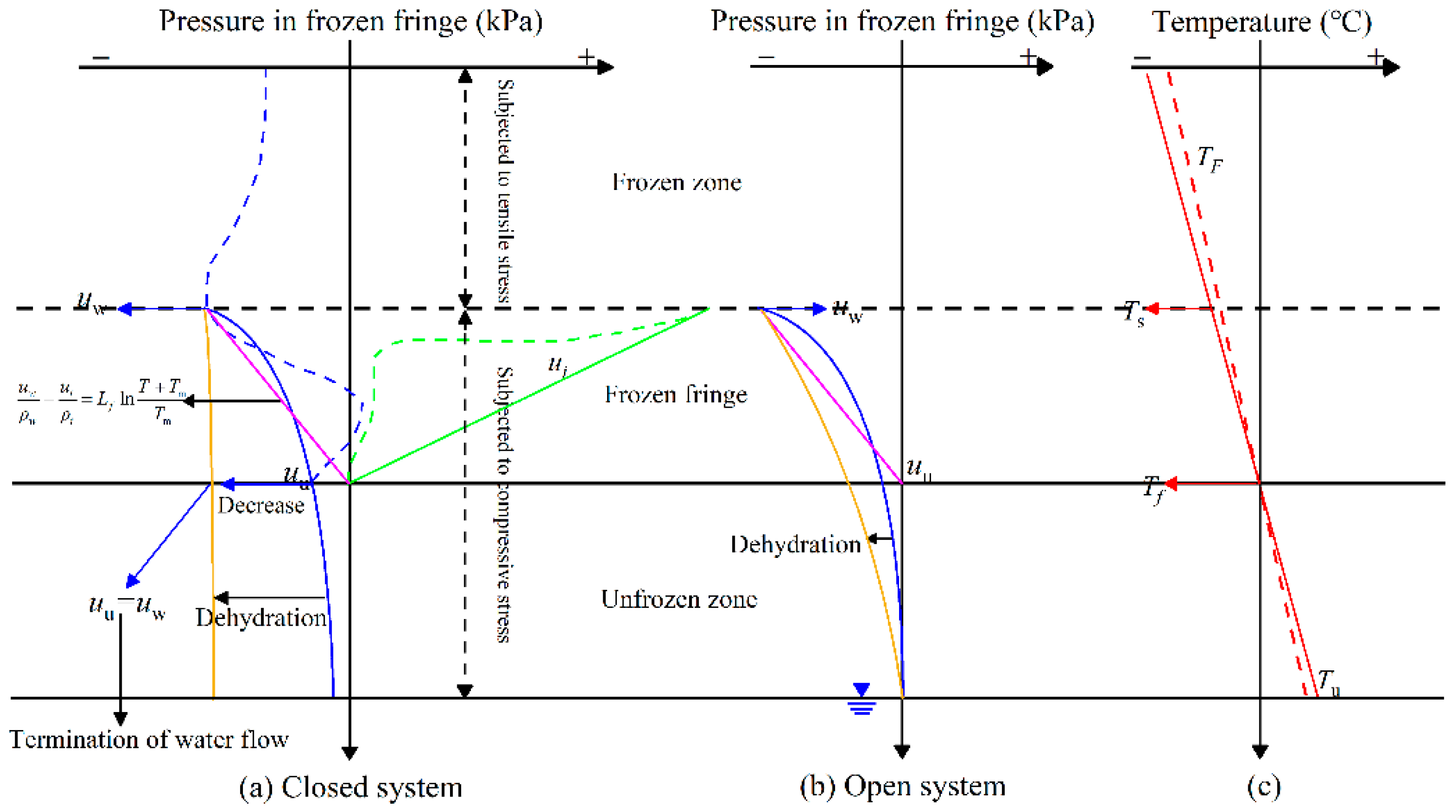
Figure 1 presents a schematic of the frost heave model. It should be noted that Figure 1 is revised from a sketch map of frozen fringe processes from Ma, et al. [17]. Figure 1a shows the pore water pressure and pore ice pressure under dynamic and steady-state conditions in an open system; Figure 1b shows the pore water pressure under steady-state conditions in a closed system; Figure 1c shows the soil temperature distribution profile under dynamic and steady-state conditions. It should be noted that the solid and dashed lines represent the steady and dynamic state, respectively. Moreover, the red, blue, green, brown and pink lines represent the soil temperature, pore water pressure, pore ice pressure, pore water pressure after dehydration and pore water pressure expressed by the Clapeyron Equation. As shown, frozen soil can be divided into frozen zones, frozen fringe zones and unfrozen zones, separated by the freezing temperature and the segregation freezing temperature. Initially, the pore water pressure of saturated unfrozen soil is positive. As the soil freezes, the pore water pressure becomes negative, during which water migrates from the unfrozen zone to the frozen fringe and accumulates and phases into ice at the base of the ice lens, resulting in a frost heave. The growth rate of ice lenses can thus be considered the rate of frost heaving. Following the mass conservation law, the growth rate of the ice lens can be determined by the water flux at the base of the ice lens. The water flux can be approximately determined by the pore water pressure gradient and the hydraulic conductivity of frozen fringes through Darcy’s law, which are all difficult to determine. Nevertheless, the segregation potential model solves this problem. However, the conventional segregation potential model considers the segregation potential to be constant and the pore water pressure at the freezing front to be zero, which is not true in a closed system. As shown in Figure 1a, in a closed system, as the water in the unfrozen zone migrates into the frozen fringe, the decrease in the water content of the unfrozen zone results in the saturated unfrozen zone becoming an unsaturated unfrozen zone and further results in a decrease in the pore water pressure at the freezing front. Therefore, the segregation potential and the pore water pressure at the freezing front should not be constant in a closed system. In addition, it should be noted that when $u_u$ is reduced to equal $u_{\mathrm{w}}$, water migration and frost heaving are terminated. In addition, as shown in Figure 1b, in some open systems, the phenomenon of dehydration similar to that of closed systems can also be observed, which should be classified as a closed system since the segregation potential and the pore water pressure at the freezing front are also not constant. Therefore, the segregation potential model is applied to freezing soil in a closed system in this study, where the segregation potential at the quasi-steady state is not a constant but varies with the water content at the freezing front. As shown in Figure 1c, the temperature in the frozen zone, frozen fringe and unfrozen soil at the quasi-steady process can be approximately viewed as linear distribution.

For freezing soils, the frost heaving phenomenon is mainly caused by water migration. The migrated water phase changes to ice at the warmest side of the ice lens; therefore, the mass conservation law is applied at this position:

$${\rho }_i{v}_i={\rho }_w{v}_w,$$

(1)

where ${\rho }_i\left(\mathrm{kg}/{\mathrm{m}}^3\right)$ and ${\rho }_w\left(\mathrm{kg}/{\mathrm{m}}^3\right)$ are the densities of ice and water, respectively, and $v_i\left(\mathrm{m}/\mathrm{s}\right)$ and $v_i\left(\mathrm{m}/\mathrm{s}\right)$ are the velocities of ice growth and water migration, respectively. Thus, the frost heave can be written as

$$h=v_{i}t=\frac{{\rho }_w}{{\rho }_i}{v}_{w}t,$$

(2)

where $t\left(\mathrm{s}\right)$ is the freezing time. The rate of water migration can be expressed by Darcy’s law,

$$v_w=-k\frac{\partial \left(u_w-u_{\mathrm{u}}\right)}{\partial x},$$

(3)

where $k\left(\mathrm{m}/\mathrm{s}\right)$ is the hydraulic conductivity of the frozen fringe, $u_w\left(\mathrm{kPa}\right)$ is the pore water pressure at the base of the ice lens and $u_u\left(\mathrm{kPa}\right)$ is the pore water pressure at the base of the frozen fringe. The negative symbol denotes that the direction of the pore water pressure is opposite to the freezing direction. In addition, the rate of water migration can also be expressed by [18]

$$v_w=SPGradT,$$

(4)

where $SP\left({\mathrm{m}}^2/\left(℃\mathrm{s}\right)\right)$ is the segregation potential and $\mathrm{Grad}T\left(℃/\mathrm{m}\right)$ is the temperature gradient. Combining Equations (3) and (4), the segregation potential can be expressed as

$$SP=k\frac{u_w-u_u}{T_s-T_f},$$

(5)

where $T_s(℃)$ is the segregation freezing temperature and $T_f(℃)$ is the freezing temperature. As shown, $k$, $u_w$, $T_s$ and $T_f$ in Equation (5) are approximately stable at the quasi-steady state. However, as the freezing time goes on, the water in the unfrozen zone will continuously migrate to the frozen fringe until $u_{\mathrm{u}}=u_{\mathrm{w}}$, resulting in a decrease in the water content in the unfrozen zone, leading to the variation of $u_u$ with freezing time. Thus, during the frost heaving process, the segregation potential expressed by Equation (5) can be revised as

$$SP\left[W_{\mathrm{f}}\left(t\right)\right]=k\frac{u_w-u_u\left[W_{\mathrm{f}}\left(t\right)\right]}{T_s-T_f},$$

(6)

where $SP\left(W_{\mathrm{f}}\right)\left({\mathrm{m}}^2/\left(℃\cdot \mathrm{s}\right)\right)$ is the revised segregation potential and $W_{\mathrm{f}}(\%)$ is the unfrozen water content at the freezing front varying with the freezing time during the dehydration process. The segregation potential is significantly affected by the external pressure and can be expressed as [19]

$$SP\left(P\right)=S{P}_0{\mathrm{e}}^{\alpha P},$$

(7)

where $SP\left(P\right)\left({\mathrm{m}}^2/\left(℃\mathrm{s}\right)\right)$ is the segregation potential under an external pressure of $P\left(\mathrm{kPa}\right)$, $S{P}_0\left({\mathrm{m}}^2/\left(℃\mathrm{s}\right)\right)$ is the initial segregation potential under no load, and $\alpha$ is the constant parameter, which can be determined from tests for various pressures. Equation (7) indicates that there exists a linear relationship between $\ln SP\left(P\right)$ and $P$; thus, Equation (7) can be rewritten as

$$SP\left(P\right)=SP\left(P_i\right){\mathrm{e}}^{\alpha \left(P-P_i\right)},$$

(8)

where $SP\left(P_i\right)$ is the segregation potential under an external pressure of $P_i\left(\mathrm{kPa}\right)$ and $P_i\left(\mathrm{kPa}\right)$ is the $i\mathrm{th}$ external pressure. It should be noted that when $P_i=0$, Equation (8) changes into Equation (7). That is, Equation (8) is the generalized relationship between the segregation potential and the external pressure. Therefore, substituting Equations (4) and (8) into Equation (2) gives the frost heave under external pressure at the quasi-steady state:

$$h\left(P\right)=\frac{{\rho }_w}{{\rho }_i}S{P}_i{\mathrm{e}}^{\alpha \left(P-P_i\right)}GradTt,$$

(9)

From Equation (9), it can be seen that the frost heave amount under external pressure, whether in an open system or closed system, can be determined by the segregation potential under external pressure, the external pressure, the temperature gradient in the frozen fringe, the freezing time and the parameter $\alpha$. Equation (9) can solve the problem of the difficult determination of the hydraulic conductivity of frozen soil, the pore water pressure difference in the frozen fringe and the thickness of the frozen fringe in the prediction of frost heave. As Equation (9) shows, the variation in frost heave amount with freezing time can be calculated on the condition that $S{P}_i$, $P_i$, $\alpha$ and $\mathrm{Grad}T$ are available, of which $S{P}_i$ can be determined by

$$S{P}_i=\frac{v\left(P_i\right)}{\mathrm{Grad}T},$$

(10)

where $v\left(P_i\right)$ can be obtained directly by the water redistribution curves at different freezing times and can be given as

$$v\left(P_i\right)=\frac{\mathrm{\Lambda }\mathrm{S}{\rho }_{\mathrm{d}}}{\mathrm{\Delta }t},$$

(11)

where $\mathrm{\Lambda }S$ is the increased area of the water redistribution curve within the interval of $\mathrm{\Delta }t\left(\mathrm{s}\right)$ and can be obtained by integrating the water redistribution curve. However, it is difficult to directly measure the water redistribution curves during the freezing process; thus, the numerical simulation method is often adopted. However, the numerical simulation method is time-consuming and laborious. In addition, $v\left(P_i\right)$ can also be indirectly obtained by

$$v\left(P_i\right)=\frac{{\rho }_i}{{\rho }_w}{h}^M\left(P_i\right),$$

(12)

where $h^M\left(P_i\right)\left(\mathrm{m}\right)$ is the frost heave under an external pressure of $P_i\left(\mathrm{kPa}\right)$ caused by water migration, $\alpha$ can be determined by tests for various pressures, and $\mathrm{Grad}T\left(℃/\mathrm{m}\right)$ can be approximately determined by the temperature gradient of the frozen soil. In an open system, $h^M$ is approximately equal to the total frost heave amount, while in a closed system, the in situ frost heave cannot be ignored; thus, $h^M\left(P_i\right)$ can be obtained by

$$h^M=h_0\left(P_i\right)-h^I\left(P_i\right),$$

(13)

where $h_0\left(P_i\right)\left(\mathrm{m}\right)$ is the total frost heave amount and $h^I\left(P_i\right)\left(\mathrm{m}\right)$ is the in situ frost heave, which can be expressed as

$$h^I\left(P_i\right)=\alpha W_0{\rho }_{\mathrm{d}}{H}_{\mathrm{f}}\left(P_i\right)\overline{W_i}\left(P_i\right),$$

(14)

where $\alpha$ is the volume expansion coefficient, $W_0(\%)$ is the initial mass water content, ${\rho }_{\mathrm{d}}\left(\mathrm{kg}/{\mathrm{m}}^3\right)$ is the dry density, $H_{\mathrm{f}}\left(P_i\right)\left(\mathrm{m}\right)$ is the frozen depth, and $\overline{W_i}\left(P_i\right)(\%)$ is the average mass ice content. The $\overline{W_i}$ can be obtained by

$$\overline{W_i}\left(P_i\right)=\frac{{\displaystyle {\int }_{T_{\mathrm{f}}\left(P_i\right)}^{T_c}{W}_i\left(P_i\right)\mathrm{d}T}}{T_{\mathrm{f}}\left(P_i\right)-T_c},$$

(15)

where $T_{\mathrm{f}}\left(P_i\right)$ is the freezing temperature, $T_c(℃)$ is the temperature of the cold end, and $W_i\left(P_i\right)$ is the mass ice content. The mass ice content can be calculated by

$$W_i\left(P_i\right)=W_0-W_u\left(P_i\right),$$

(16)

where $W_u\left(P_i\right)$ is the mass unfrozen water content and can be determined from the experiment. The effect of external pressure on the freezing point can be given as [20]

$$T_f\left(P_i\right)=T_{f0}+\frac{1-\beta }{\eta }{P}_i,$$

(17)

where $T_{f0}\left(\mathrm{K}\right)$ is the freezing point under no load, $\beta =1.09$ and $\eta =1.23\mathrm{MPa}/℃$. The effect of external pressure on the unfrozen water content can be given as [20]

$$W_u\left(P_i\right)=A{\left[-T+T_{f0}+\frac{1-\beta }{\eta }{P}_i+{\left(\frac{W_0}{A}\right)}^{\frac{1}{B}}\right]}^B,$$

(18)

where $T\left(\mathrm{K}\right)$ is the temperature of the soil sample and A and B are the parameters that can be obtained from the soil freezing characteristic curve under no load.

3. Frost Heaving Test

3.1. Material and Method

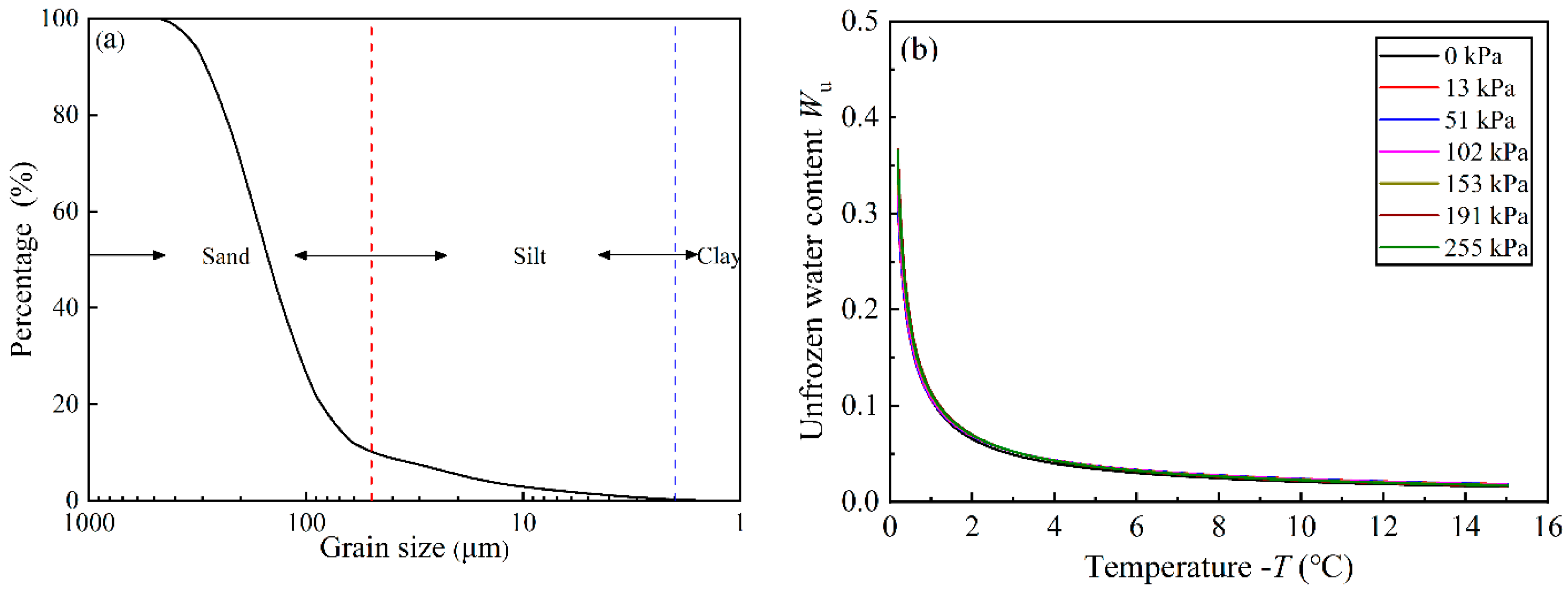
The soil sample studied in this paper was collected from Heihe, China. The soil properties are summarized in

Table 1. Properties of the soil samples.

$\mathit{L}\left(\mathbf{mm}\right)$	$\mathit{D}\left(\mathbf{mm}\right)$	${\mathit{W}}_{\mathit{L}}$	${\mathit{W}}_{\mathit{P}}$	${\mathit{W}}_{\mathbf{i}}$	${\mathit{\rho }}_{\mathbf{d}}\left(\mathbf{kg}/{\mathbf{m}}^3\right)$	${\mathit{T}}_{\mathbf{f}}(℃)$	Sand (%)	Silt (%)	$\mathbf{Clay}(\%)$
110	100	0.351	0.228	0.351	1.43	−0.18	89.8	9.92	0.28

. According to the USDA soil texture triangle [21], the soil can be defined as sand. Figure 2a shows the accumulative curve of particle size grading of the soil sample. Figure 2b shows the soil freezing characteristic curve (SFCC) of the soil sample, describing the relation between the subfreezing temperature and the unfrozen water content, which was obtained in the laboratory through nuclear magnetic resonance (NMR) technology. As shown, the unfrozen water content decreases exponentially with decreasing negative temperature and decreases dramatically within −1 °C. This phenomenon can be explained by the fact that a large amount of capillary water in the soil is prone to freezing, while a small amount of bound water is resistant to freezing.

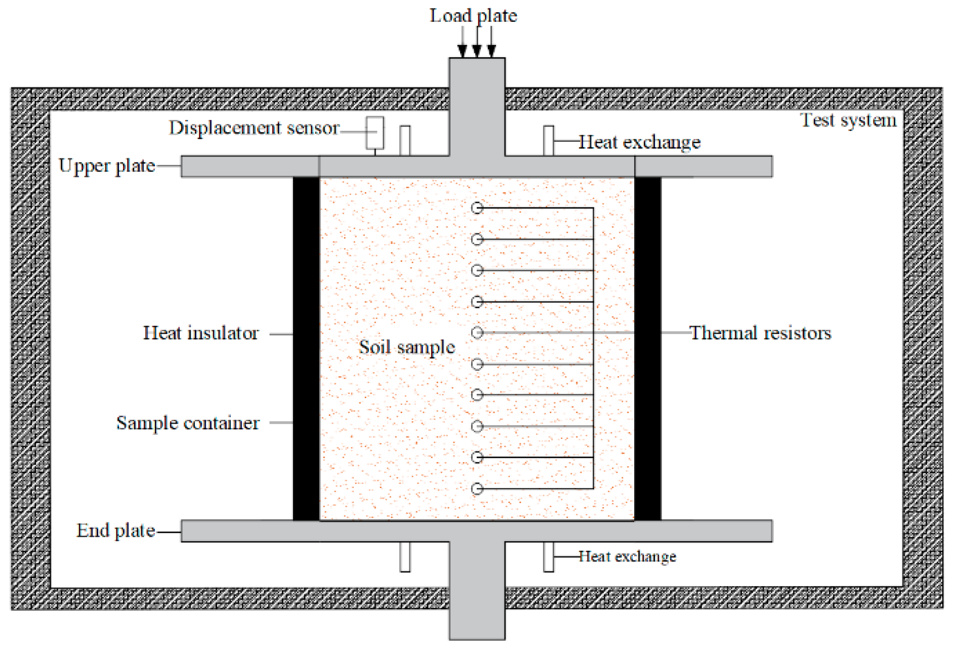
The freezing–thawing test chamber located in the State Key Laboratory of Frozen Soil Engineering was used for this study, a schematic of which is shown in Figure 3. In the freezing–thawing test chamber, the outside chamber was used to control the ambient temperature of the soil sample, the alcohol circulating in the top and end plates was used to cool the top and bottom of the soil sample, the displacement meter placed on the top cooling end was used to measure the frost heave, and the thermal resistors inserted in the soil sample were used to measure the soil temperature.

The experimental procedure can be summarized as follows: (1) Preparation of the soil sample. The air-dried soil was mixed with pure water, packed into the soil container and saturated in the vacuum saturator. (2) Installation of the soil sample. The prepared soil sample container was wrapped with an insulator, and 10 holes were reserved to insert the thermal resistors. The soil container was placed between the bottom and top temperature control plates, the bolts were tightened, and then the displacement meter was installed on the top plate. (3) Initiation of the experiment. The thermostat door was closed, and the temperature of the top and bottom plates was set to 1 °C. After the soil temperature was stable for 8 h, the temperature of the top plate was set to −2 °C for 72 h. The desired pressures were applied during the whole test. No water was allowed to enter or discharge during the entire experimental process. During this time, compression tests of unfrozen soil under the same conditions as the frost heaving tests were carried out since the unfrozen zone of the frozen soil will be compressed during the frost heaving process. The experimental conditions are summarized in

Table 2. Experimental conditions.

Test Number	External Pressure	Controlled Temperature (°C)
		Cool End	Warm End
P1-P7	0, 13, 51,102, 153, 191, 255 (kPa)	−2	1
P1-P7	0, 13, 51,102, 153, 191, 255 (kPa)	20

.

3.2. Test Results

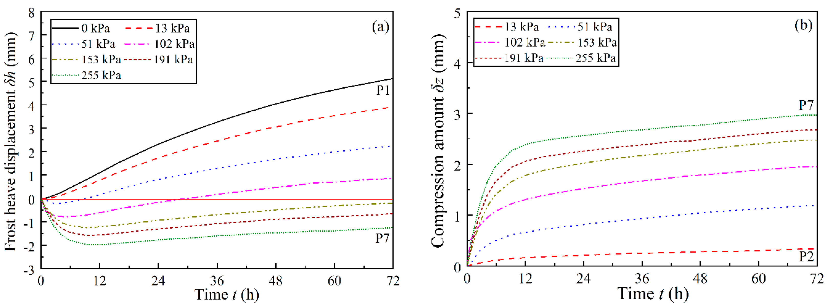
Figure 4a shows the frost heave displacement under the constant external pressures measured directly by the displacement meter. As shown, the frost heave displacement under no load increased with the freezing time, while the frost heave displacement under the external pressures decreased first and then increased with the freezing time because the soil samples were compressed under the external pressures during the frost heaving process. In addition, the frost heave displacement decreased with increasing external pressure, and compression instead of swelling was found when the pressure increased to 153 kPa because the amount of frost heave displacement was less than the amount of compression. Figure 4b shows the amount of compression for the unfrozen zone under the external pressures, which was approximately calculated by the compressive modulus and the length of the unfrozen zone. It should be noted that the compression of the frozen zone was neglected. As shown, the amount of compression increased rapidly within 6 h, which was consistent with the results of the frost heaving test shown in Figure 4a. Moreover, the increasing amount of compression shown in Figure 4b was close to the decreasing frost heave displacement in Figure 4a; thus, the frost heave amount can also be obtained by subtracting the decreasing frost heave displacement. In addition, the compression amount increased with increasing external pressures, which was similar to the result in Figure 4a.

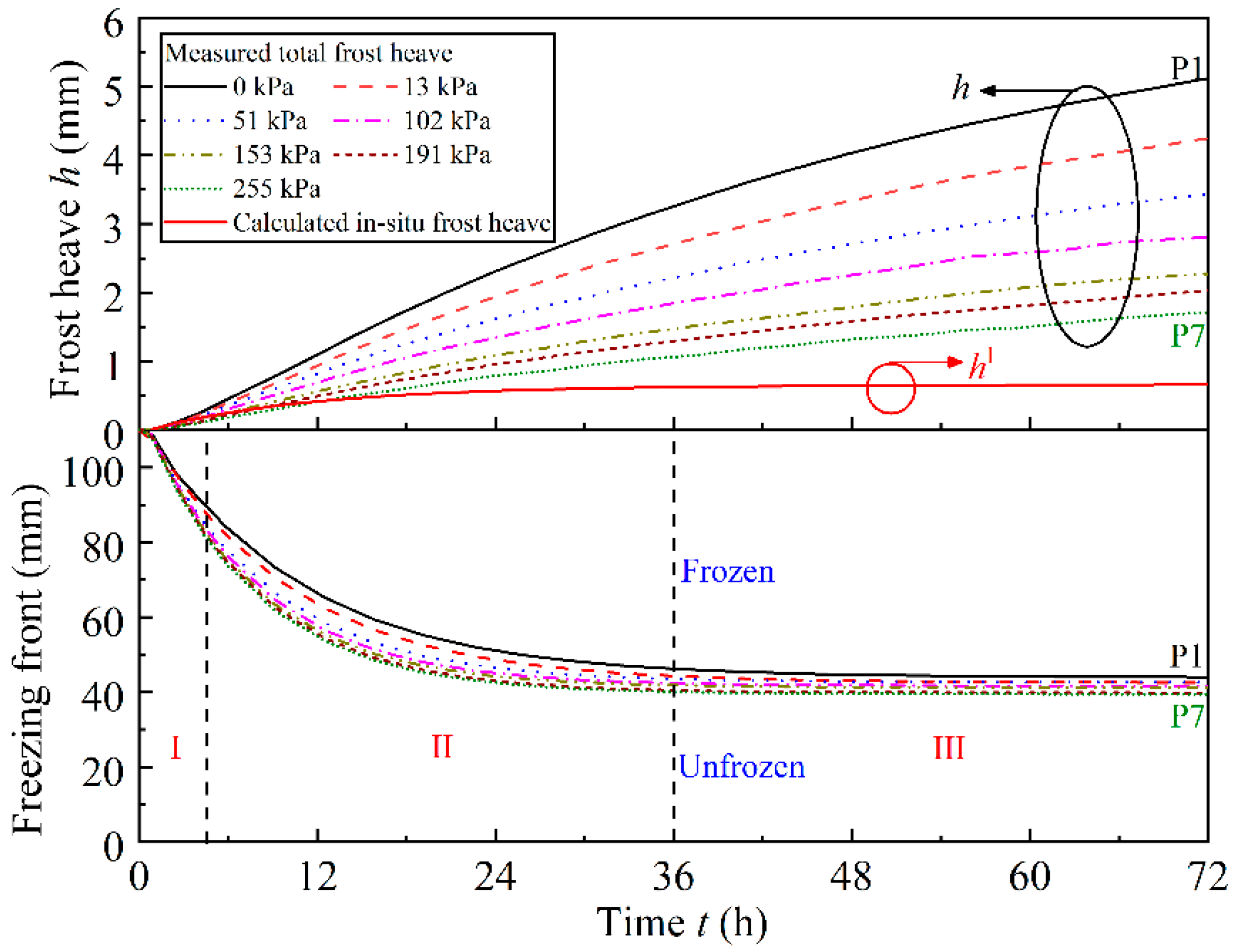
Figure 5 shows the variation of the frost heave amount and freezing front position with freezing time under external pressures. As shown, the frost heave amount and the frozen depth under the external pressures increase with the freezing time as a power function [22],

$$h\mathrm{or}{H}_f=a{t}^b+c,$$

(19)

where h (mm) is the frost heave, H_f (mm) is the frozen depth, t (h) is the freezing time, and a and b are constant parameters. Moreover, the frost heave amount was found to decrease with increasing external pressure owing to the external pressure delay of water migration [14], while the frozen depth was found to increase with increasing external pressure [23] because the unfrozen zone was compressed by the external pressure. In addition, the development of the freezing front can be divided into (I) a fast-freezing stage, during which the soil water is frozen in situ without migration, resulting in a small amount of frost heave and a very slow frost heave curve; (II) a transition stage, during which the water begins to migrate from the unfrozen zone to the frozen zone owing to the decrease of the freezing rate, resulting in an increase in the frost heave amount and the formation of a small amount of ice; and (III) a quasi-steady stage, during which more water migrates from the unfrozen zone to the frozen zone owing to the freezing rate varying very slowly, resulting in the formation of a large amount of ice. This phenomenon was consistent with previous studies [24].

3.3. Calculation of Segregation Potential from the Frost Heaving Test

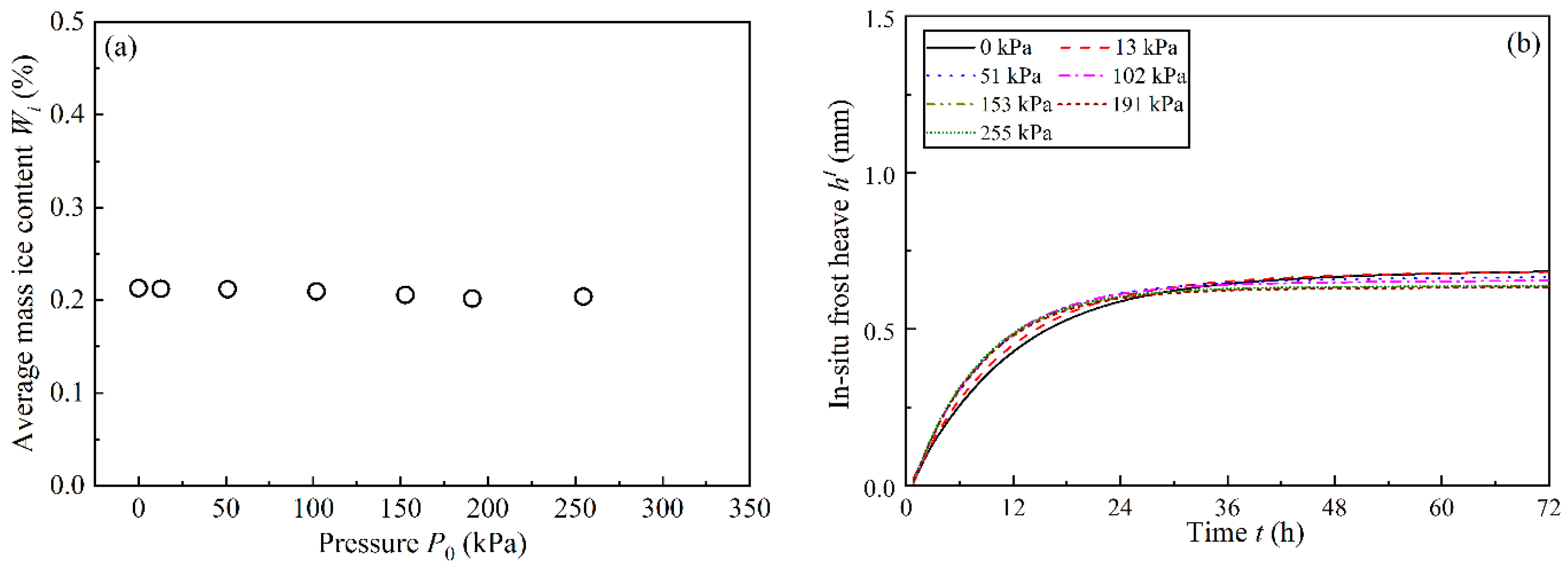
Figure 6a shows the variation of average mass ice content with the external pressure, which was calculated by Equations (15)–(18). As shown, the average mass ice content decreases with increasing external pressure. This can be explained by the fact that the external pressure reduced the segregation freezing temperature, inhibiting the growth of the ice lens. Figure 6b shows the in situ frost heave calculated by Equation (14) by means of the results of Figure 6a. As shown, the final in situ frost heave also decreased with increasing external pressure, which can be attributed to the same reason as the average mass ice content. In addition, it can be found that the in-situ frost heave was far less than the total frost heave, which can be seen from Figure 5. The result indicates that the frost heave caused by water migration played a key role in the total frost heave.

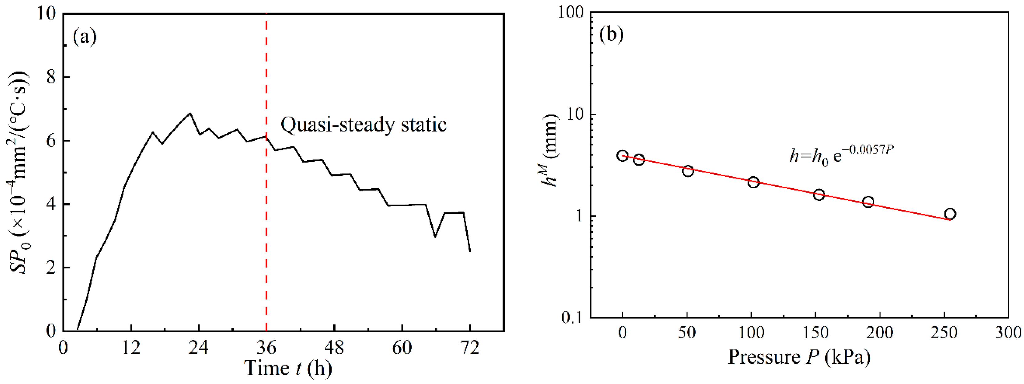
Figure 7a shows the initial segregation potential calculated by the frost heave caused by water migration, which was calculated by the measured total frost heave and the calculated in situ frost heave. As shown, the segregation potential increases first and then decreases with freezing time. It can be seen that the segregation potential is not a constant, even at a quasi-steady state, which is not consistent with the conventional segregation potential. It should be noted that the segregation potential at the transient state was also analyzed, the objective of which was to understand the variation of the segregation potential over the whole freezing time. Figure 7b shows the relationship of the final frost heave with the external pressure, which was used to determine the parameter $\alpha$. As shown, the final frost heave decreases linearly with the increase of the external pressure in the ln h-P₀ coordinates, and the slope is the parameter $\alpha$.

4. Determination of the Segregation Potential from Numerical Simulation Results

To illustrate the rationality of calculating the segregation potential from the frost heaving test, the numerical simulation method adopted in this section was used to simulate the water redistribution curves at different freezing times, the result of which was then used to obtain the water migration rate to calculate the segregation potential, which was further compared with that calculated from the frost heave test.

4.1. Simulation Method

4.1.1. Assumption

To employ the hydrothermal coupling model, the following items are assumed:

(1)

Darcy’s law is applicable for water migration during the soil freezing processes.

(2)

The soil in the study is isotropic and elastic.

4.1.2. Equilibrium Equations

The water and heat distribution can be obtained by simultaneously solving the mass conservation equation and the energy balance equation [25,26]:

$$\frac{\partial {\theta }_u}{\partial t}+\frac{{\rho }_i}{{\rho }_w}\cdot \frac{\partial {\theta }_i}{\partial t}=\nabla \left[D\left({\theta }_u\right)\nabla {\theta }_u+k\left({\theta }_u\right)\right],$$

(20)

$$C\left(\theta \right)\frac{\partial T}{\partial t}=\lambda \left(\theta \right){\nabla }^{2}T+L\cdot {\rho }_i\frac{\partial {\theta }_i}{\partial t},$$

(21)

where

$$D\left({\theta }_u\right)=\frac{k\left({\theta }_u\right)}{c\left({\theta }_u\right)}\cdot I,$$

(22)

$$I={10}^{-10{\theta }_i},$$

(23)

where ${\theta }_u\left({\mathrm{cm}}^3/{\mathrm{cm}}^3\right)$ is the volumetric unfrozen water content, $k\left(\mathrm{m}/\mathrm{s}\right)$ is the hydraulic conductivity, $D\left({\theta }_u\right)\left({\mathrm{m}}^2/\mathrm{s}\right)$ is the thermal diffusivity, $T(℃)$ is the soil temperature, $t\left(\mathrm{s}\right)$ is the time, ${\theta }_i\left({\mathrm{cm}}^3/{\mathrm{cm}}^3\right)$ is the volumetric ice content, ${\rho }_i\left(\mathrm{kg}/{\mathrm{m}}^3\right)$ is the density of ice, $L\left(\mathrm{kJ}/\mathrm{kg}\right)$ is latent heat, $\lambda \left(\theta \right)\left(\mathrm{W}/\left(\mathrm{m}\cdot ℃\right)\right)$ is the thermal conductivity, $C\left(\theta \right)\left({\mathrm{kJ}/\mathrm{m}}^3\right)$ is the volumetric heat capacity, and $I$ is the ice resistance. Since the three unknown quantities of soil temperature, volumetric ice content and volumetric unfrozen water content exist in the two governing equations, a relation equation was introduced to solve the hydrothermal coupling model:

$${\theta }_i=B_i\left(T\right)\cdot {\theta }_u,$$

(24)

where

$$B_i=\frac{{\theta }_i}{{\theta }_u}=\{\begin{array}{l}1.1\left[{\left(\frac{T}{T_f}\right)}^A-1\right] \left(T<T_f\right)\\ 0 \left(T\ge T_f\right)\end{array},$$

(25)

where $B_i\left(T\right)$ is the ratio of the volumetric ice content and the unfrozen water content.

4.2. Simulation Results

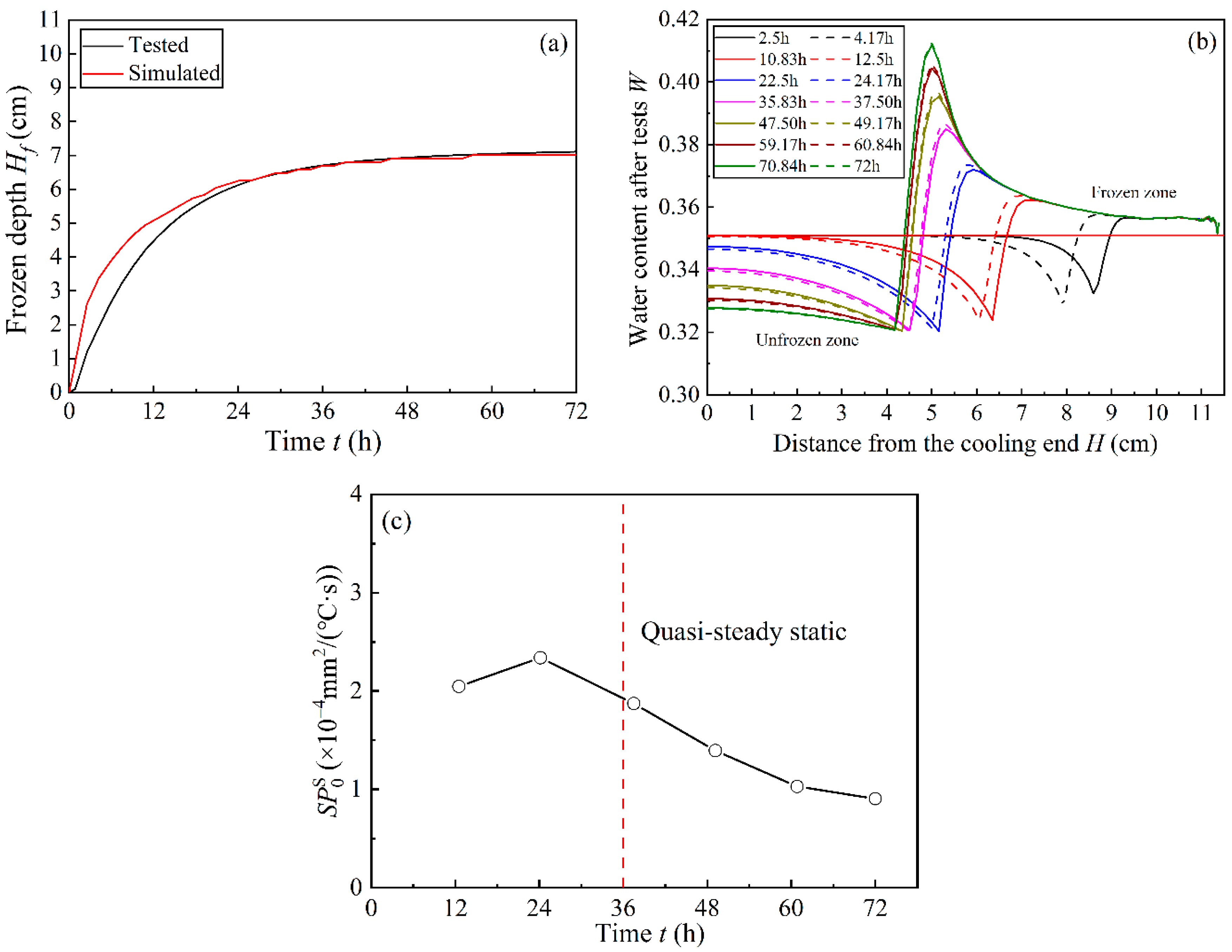
Figure 8a presents a comparison of the simulated frozen depth with the measured frozen depth under no load. As shown, the simulated frozen depth was in good agreement with the measured frozen depth. Figure 8b presents the simulated water redistribution of the soil samples at different freezing times under no load. As shown, the water content in unfrozen soil decreased, while the water content in frozen soil increased with increasing time. It can be concluded that the water in the unfrozen zone evidently migrated to the frozen zone, which was the main reason for the frost heave. Figure 8c presents the variation of $S{P}_0^{\mathrm{S}}$ with freezing time. It should be noted that the $S{P}_0^{\mathrm{S}}$ was calculated by the water migration rate obtained by the water redistribution profile in Figure 8b. As shown, $S{P}_0^{\mathrm{S}}$ changes similarly with $S{P}_0^{\mathrm{M}}$, which increases first and then decreases with freezing time.

5. Approach to Applying the Segregation Potential Model in Closed Systems

To illustrate the rationality of calculating the segregation potential from the frost heaving test, the segregation potential calculated from the numerical simulation results was compared with that calculated from the frost heaving test. Then, the segregation potential calculated from the frost heaving test was used to calculate the frost heave to illustrate the possibility of applying the segregation potential model in a closed system.

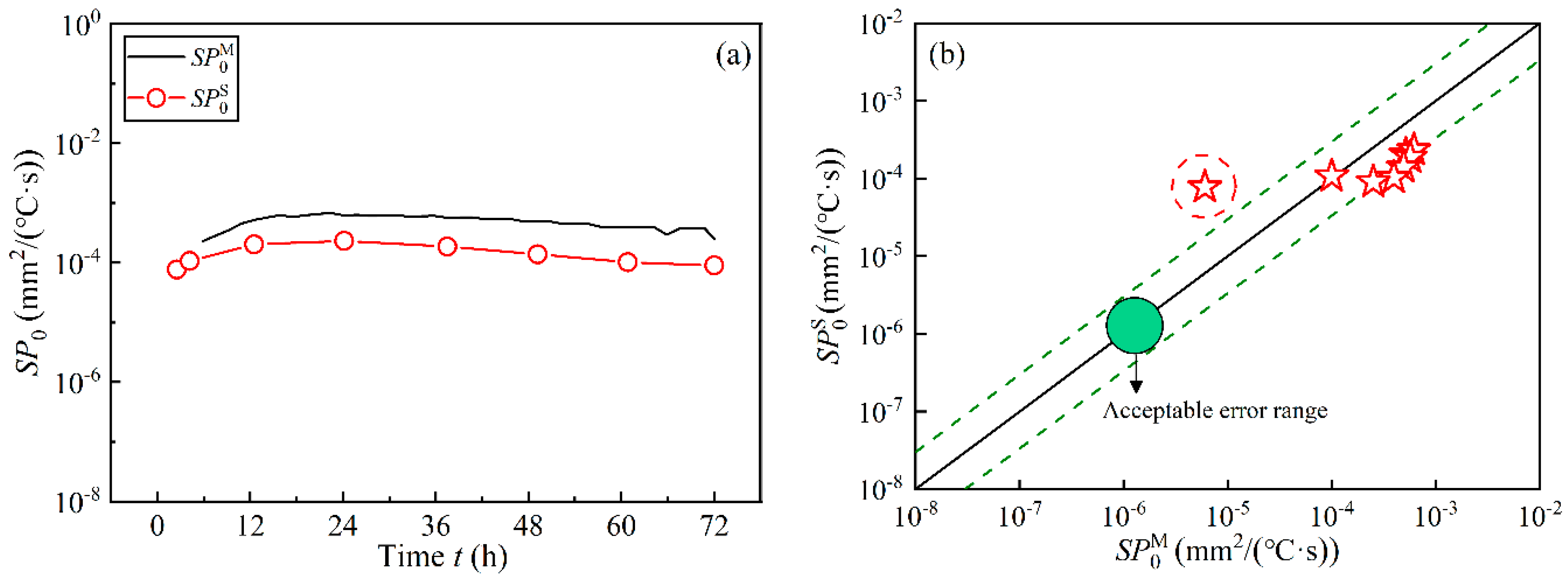
5.1. Comparison of the $S{P}_0^{\mathrm{M}}$ and $S{P}_0^{\mathrm{S}}$

Figure 9 shows a comparison of $S{P}_0^{\mathrm{M}}$ and $S{P}_0^{\mathrm{S}}$. As shown, the black line represents $S{P}_0^{\mathrm{M}}$, while the red line represents $S{P}_0^{\mathrm{S}}$. As shown, $S{P}_0^{\mathrm{M}}$ was close to $S{P}_0^{\mathrm{S}}$ but slightly overestimated $S{P}_0^{\mathrm{S}}$. However, the overall performance of the proposed model was acceptable, as shown in Figure 9b. It should be noted that the zone between the green dashed lines represents the acceptable error range, which was in the range of $\left(S{P}_0^{\mathrm{M}}+2\times {10}^{-n},S{P}_0^{\mathrm{M}}-2\times {10}^{-n}\right)$ [27]. As shown, all the data points except the point at the freezing time of 2.5 h are located in the acceptable error range, which can be accepted since the state at the freezing time of 2.5 h is still unsteady. Thus, it can be concluded that estimating the segregation potential from the frost heave test was reasonable and simple.

5.2. Applying the Segregation Potential Model in a Closed System

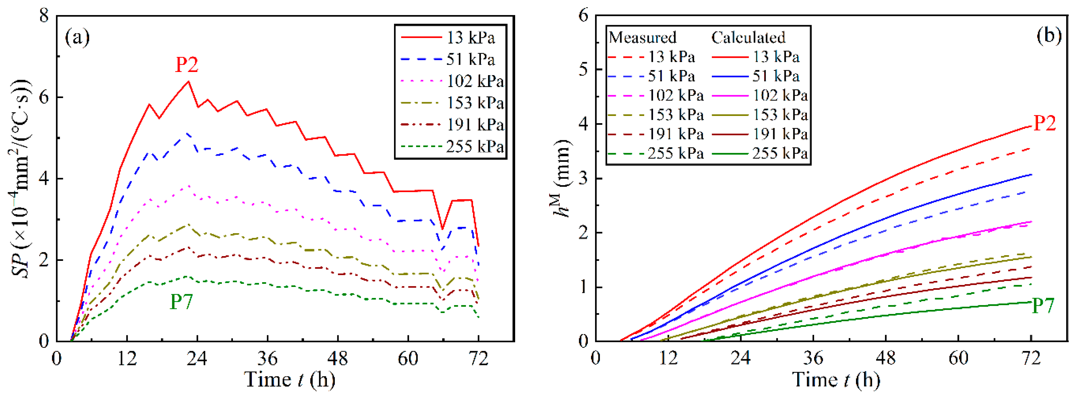
To illustrate the possibility of applying the segregation potential model in a closed system, the segregation potential calculated from the frost heaving test was used to calculate the frost heave, which was further compared with the test data. Figure 10a shows the segregation potential under the external pressure calculated by Equation (7) by means of Figure 7. As shown, the segregation potential under the external pressure exhibits a similar trend to the potential under no load. Figure 10b gives the frost heave amount calculated by Equation (9) by means of Figure 10a, which was further compared with the measured frost heave amount. As shown, the calculated values fit the measured data well, which shows the applicability of the model in a closed system.

Besides, the root mean square error (RMSE) was calculated to illustrate the model performance [28].

$$\mathrm{RMSE}=\sqrt{\frac{{\displaystyle \sum _{i=1}^N{\left(h_p-h_t\right)}^2}}{N}},$$

(26)

where $h_{\mathrm{p}}\left(\mathrm{m}\right)$ and $h_{\mathrm{t}}\left(\mathrm{m}\right)$ are the predicted and tested frost heave, respectively; $i$ is the count of the current data points and $N$ is the number of data points. The calculated values of RMSE at different external pressures are summarized in

Table 3. Root mean square errors (RMSEs) of the soil samples.

$\mathit{P}$(kPa)	RMSE	Average
13	0.26	0.13
51	0.19
102	0.02
153	0.04
191	0.11
255	0.18

. As shown, the average RMSE is very small, which thus indicates that the model performs well.

5.3. Further Validation of the Model in a Closed System

To further verify the validity of the model, the existing frost heaving test data in the literature of Lai, Pei, Zhang and Zhou [14], Zhang, et al. [29] and Ming, et al. [30] were further applied in this study. It should be noted that the experiments were carried out in an open system, and the phenomenon of dehydration was also observed in the unfrozen zone; thus, the experiments should be classified into a closed system.

Table 4. Experimental conditions.

References	$\mathit{P}$ (kPa)	${\mathit{T}}_{\mathbf{c}} (℃)$	${\mathit{T}}_{\mathit{w}} (℃)$	${\mathit{W}}_0 (\%)$	$\mathbf{Grad}\mathit{T} \left(℃/\mathbf{cm}\right)$
[14]	50	−1.6	1.5	20.59	0.31
	100	−1.6	1.5	20.52	0.31
[29]	50	−2.0	2.0	22.30	0.36
	150	−2.0	2.0	22.34	0.36
	300	−2.0	2.0	22.37	0.36
	500	−2.0	2.0	22.16	0.36
[30]	0	−2.0	3.0	16.02	0.50
	100	−2.0	3.0	16.34	0.50
	200	−2.0	3.0	16.17	0.50

summarizes the experimental conditions.

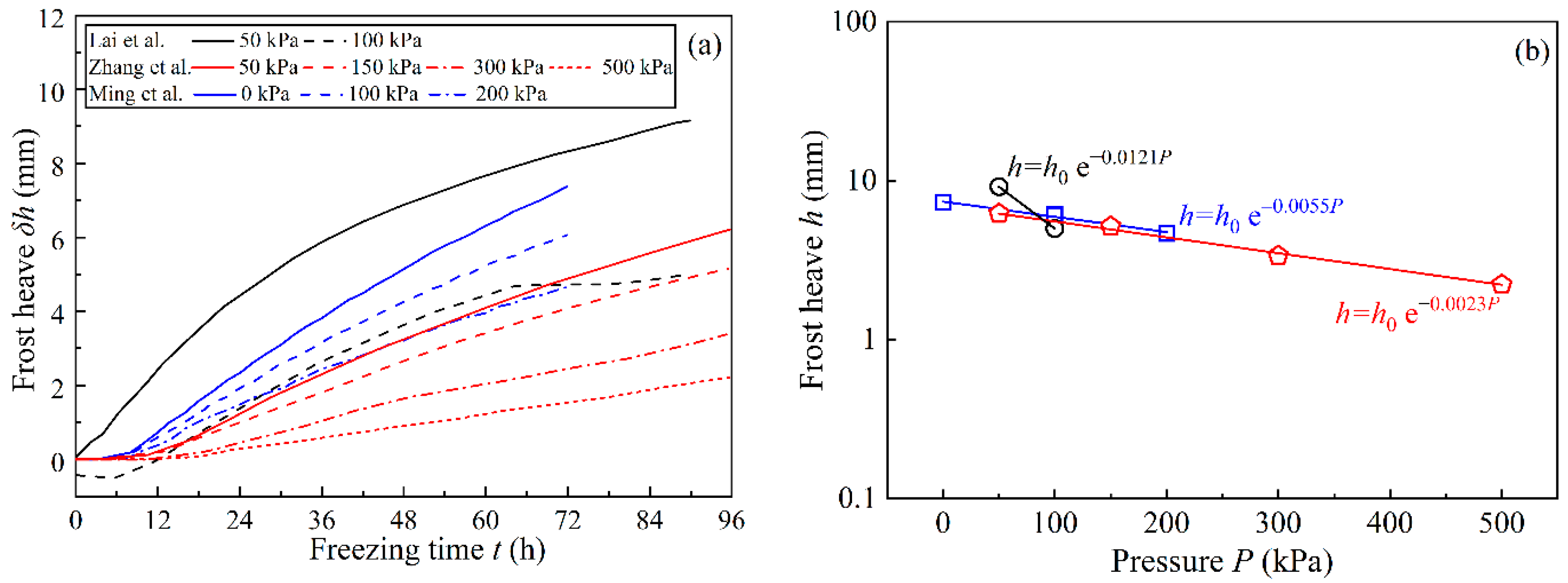
Figure 11a presents the frost heave amount under the external pressure. As shown, the frost heave decreases with the increasing external pressure which is consistent with our results. Figure 11b gives the relationship of frost heave with the external pressure, which was used to determine the parameter $\alpha$.

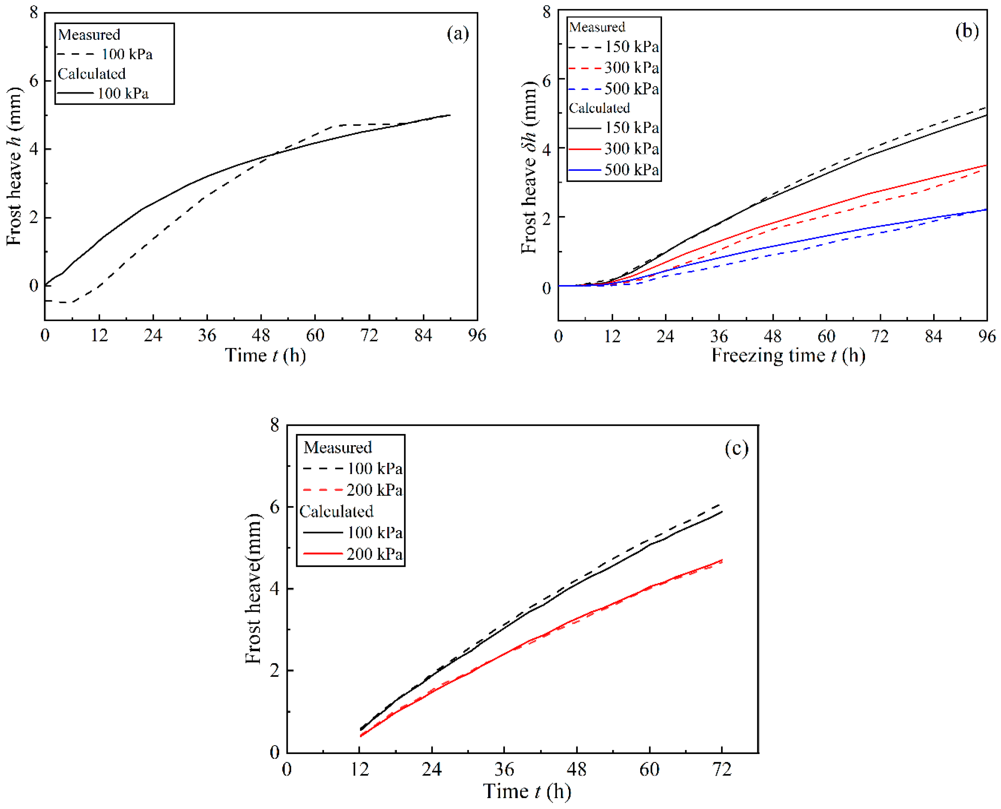
Figure 12 gives the frost heave amount calculated by Equation (9), which was further compared with the measured frost heave amount. As shown, the calculated values fit the measured data well, which further shows the availability of the model. Besides, the RMSEs of the three soil samples were calculated to illustrate the model performance and summarized in

Table 5. RMSEs of the three soil samples.

References	$\mathit{P}$ (kPa)	RMSE	Average
[14]	100	0.67	0.67
[29]	150	0.13	0.17
	300	0.22
	500	0.17
[30]	100	0.12	0.08
	200	0.05

. As shown, the RMSE of the soil sample from Lai et al. [14] is relatively high, and the RMSEs of the soil sample from Zhang et al. [29] and Ming et al. [30] are very small, which indicates that the model performs well for the soil sample from Lai et al. [14], while it performs better for the soil samples from Zhang et al. [29] and Ming et al. [30] Besides, the results also show that the more measured segregation potential data points under external pressures used, the better the model performs.

Although the segregation potential model can be successfully applied in the closed system, there still exit some limitations in the model. First, the quantitative relationship between the segregation potential and the characteristics of frozen fringes is not given in this study. Second, measuring the variation of segregation potential with freezing time is required in the model. Nevertheless, the comparison of the numerical simulation and experimental results and the analysis of three existing experiments have further confirmed the application prospects of the model.

6. Conclusions

This study extends the segregation potential model to freezing soil in a closed system, where the segregation potential at the quasi-steady state is not a constant. The segregation potential at the quasi-steady state in the closed system varies with the water content at the freezing front since the pore water pressure varies with the water content at the freezing front owing to the dehydration of the unfrozen zone, based on the consideration of which the extended application of segregation potential in the closed system was attempted. The possibility of the application of the segregation potential model in a closed system was illustrated by comparing the experimental results and the numerical simulation results.

References

- Kraatz, S.; Jacobs, J.M.; Miller, H.J. Spatial and temporal freeze-thaw variations in Alaskan roads. Cold Reg. Sci. Technol. 2019, 157, 149–162. [Google Scholar] [CrossRef]
- Wu, X.Y.; Niu, F.J.; Lin, Z.J.; Luo, J.; Zheng, H.; Shao, Z.J. Delamination frost heave in embankment of high speed railway in high altitude and seasonal frozen region. Cold Reg. Sci. Technol. 2018, 153, 25–32. [Google Scholar] [CrossRef]
- Wang, Y.P.; Jin, H.J.; Li, G.Y. Investigation of the freeze-thaw states of foundation soils in permafrost areas along the China–Russia Crude Oil Pipeline (CRCOP) route using ground-penetrating radar (GPR). Cold Reg. Sci. Technol. 2016, 126, 10–21. [Google Scholar] [CrossRef]
- Yang, Z.H.; Dutta, U.; Xiong, F.; Biswas, N.; Benz, H. Seasonal frost effects on the dynamic behavior of a twenty-story office building. Cold Reg. Sci. Technol. 2008, 51, 76–84. [Google Scholar] [CrossRef]
- Qin, Z.P.; Lai, Y.M.; Tian, Y.; Yu, F. Frost-heaving mechanical model for concrete face slabs of earthen dams in cold regions. Cold Reg. Sci. Technol. 2019, 161, 91–98. [Google Scholar] [CrossRef]
- Miller, R.D. Lens initiation in secondary heaving. In Proceedings of the International Symposium on Frost Action in Soils, Luleå, Sweden, 16–18 February 1977. [Google Scholar]
- O’Neill, K.; Miller, R.D. Exploration of a rigid ice model of frost heave. Water Resour. Res. 1985, 21, 281–296. [Google Scholar] [CrossRef]
- Michalowski, R.L.; Zhu, M. Frost heave modelling using porosity rate function. Int. J. Numer. Anal. Methods Geomech. 2006, 30, 703–722. [Google Scholar] [CrossRef] [Green Version]
- Chen, L.; Zhang, X.Y. A model for predicting the hydraulic conductivity of warm saturated frozen soil. Build. Sci. 2020, 179, 106939. [Google Scholar] [CrossRef]
- Edlefsen, N.E.; Anderson, A.B.C. Thermodynamics of soil moisture. Hilgardia 1943, 12, 117–123. [Google Scholar] [CrossRef] [Green Version]
- Miyata, Y.; Akagawa, S. An experimental study of dynamic solid-liquid phase equilibrium in a poroius medium. JSME Int. J. Ser. B 1998, 41, 590–600. [Google Scholar] [CrossRef] [Green Version]
- Bronfenbrener, L.; Bronfenbrener, R. Modeling frost heave in freezing soils. Cold Reg. Sci. Technol. 2010, 61, 43–64. [Google Scholar] [CrossRef]
- Zhou, J.Z.; Li, D.Q. Numerical analysis of coupled water, heat and stress in saturated freezing soil. Cold Reg. Sci. Technol. 2012, 72, 43–49. [Google Scholar] [CrossRef]
- Lai, Y.M.; Pei, W.S.; Zhang, M.Y.; Zhou, J.Z. Study on theory model of hydro-thermal-mechanical interaction process in saturated freezing silty soil. Int. J. Heat Mass Transf. 2014, 78, 805–819. [Google Scholar] [CrossRef]
- Konrad, J.M.; Morgenstern, N.R. The segregation potential of a freezing soil. Can. Geotech. J. 1981, 18, 482–491. [Google Scholar] [CrossRef]
- Nixon, J.F. Field frost heave predictions using the segregation potential concept. Can. Geotech. J. 1982, 19, 526–529. [Google Scholar] [CrossRef]
- Ma, W.; Zhang, L.; Yang, C. Discussion of the applicability of the generalized Clausius–Clapeyron equation and the frozen fringe process. Earth Sci. Rev. 2015, 142, 47–59. [Google Scholar] [CrossRef]
- Konrad, J.M.; Morgenstern, N.R. A mechanistic theory of ice lens formation in fine-grained soils. Can. Geotech. J. 1980, 17, 473–486. [Google Scholar] [CrossRef]
- Konrad, J.M.; Morgenstern, N.R. Frost heave prediction of chilled pipelines buried in unfrozen soils. Int. J. Rock Mech. Min. Sci. Geomech. Abstr. 1984, 21, 100–115. [Google Scholar] [CrossRef]
- Zhou, J.Z.; Wei, C.F.; Lai, Y.M.; Wei, H.Z.; Tian, H.H. Application of the generalized clapeyron equation to freezing point depression and unfrozen water content. Water Resour. Res. 2018, 54, 9412–9431. [Google Scholar] [CrossRef]
- Campbell, G.S. Soil Physics with Basic: Transport Models for Soil-Plant Systems; Elsevier: Amsterdam, The Netherlands, 1985; Volume 14. [Google Scholar]
- Xu, X.Z.; Wang, J.C.; Zhang, L.X. Frozen Soil Physics Science; Science Press: Beijing, China, 2010. [Google Scholar]
- Sheng, D.C.; Zhang, S.; Yu, Z.W.; Zhang, J.S. Assessing frost susceptibility of soils using PCHeave. Cold Reg. Sci. Technol. 2013, 95, 27–38. [Google Scholar] [CrossRef] [Green Version]
- Ji, Y.K.; Zhou, G.Q.; Zhao, X.D.; Wang, J.Z.; Wang, T.; Lai, Z.J.; Mo, P.Q. On the frost heaving-induced pressure response and its dropping power-law behaviors of freezing soils under various restraints. Cold Reg. Sci. Technol. 2017, 142, 25–33. [Google Scholar] [CrossRef]
- Harlan, R.L. Analysis of coupled heat-fluid transport in partially. Water Resour. Res. 1973, 9, 1314–1323. [Google Scholar] [CrossRef] [Green Version]
- Taylor, G.S.; Luthin, J.N. A model for coupled heat and moisture transfer during soil freezing. Can. Geotech. J. 1978, 15, 548–555. [Google Scholar] [CrossRef]
- Ming, F.; Chen, L.; Li, D.Q.; Wei, X.B. Estimation of hydraulic conductivity of saturated frozen soil from the soil freezing characteristic curve. Sci. Total Environ. 2020, 698, 134132. [Google Scholar] [CrossRef]
- Lebeau, M.; Konrad, J.M. A new capillary and thin film flow model for predicting the hydraulic conductivity of unsaturated porous media. Water Resour. Res. 2010, 46. [Google Scholar] [CrossRef]
- Zhang, X.Y.; Zhang, M.Y.; Lu, J.G.; Pei, W.S.; Yan, Z.R. Effect of hydro-thermal behavior on the frost heave of a saturated silty clay under different applied pressures. Appl. Therm. Eng. 2017, 117, 462–467. [Google Scholar] [CrossRef]
- Ming, F.; Zhang, Y.; Li, D.Q. Experimental and theoretical investigations into the formation of ice lenses in deformable porous media. Geosci. J. 2016, 20, 667–679. [Google Scholar] [CrossRef]
Figure 1.
Schematic diagram of the frost heave model. (a) Open system, (b) Closed system, (c) Temperature distribution in closed system and open system. The solid lines represent the quasi-static state, and the dashed lines represent the dynamic state. The blue lines represent the pore water pressure, the pink line represents the pore water pressure expressed by the Clapeyron Equation, the brown line represents the pore water pressure in the case of terminated water flow, the green lines represent the pore ice pressure, and the red lines represent the soil temperature.
Figure 2.
(a) Accumulative curve of particle size grading of soil samples, (b) soil freezing characteristic curve of soil sample.
Figure 3.
Schematic of the experimental apparatus.
Figure 4.
Variations in the frost heave displacement (a) and compression amount with freezing time under external pressures (b).
Figure 5.
Variations of real frost heave and freezing front with freezing time under external pressures.
Figure 6.
(a) Variations of the average mass ice content with external pressure, (b) variation of in situ frost heave with freezing time under external pressures.
Figure 7.
(a) Variation of segregation potential under no load with the freezing time, (b) variation of final frost heave with the external pressure.
Figure 8.
(a) Comparison of simulated and measured frozen depth under no load, (b) profile of water redistribution of the soil samples at different freezing times under no load, (c) variation of the segregation potential with the freezing time.
Figure 9.
(a) Variation of the and the with the freezing time, (b) comparison of initial segregation potential calculated by measured data and the simulated data.
Figure 10.
(a) Segregation potential under external pressure calculated by Equation (7), (b) comparison of calculated and measured frost heave amounts.
Figure 11.
(a) Variation of frost heave under external load with the freezing time, (b) variation of final frost heave with the external pressure.
Figure 12.
Comparison of the calculated and measured frost heave from (a) Lai et al. [14], (b) Zhang et al. [29], (c) Ming et al. [30].