
Comparing Methods of Calculating Expected Annual Damage in Urban Pluvial Flood Risk Assessments

Abstract
:
1. Introduction
2. Materials and Methods
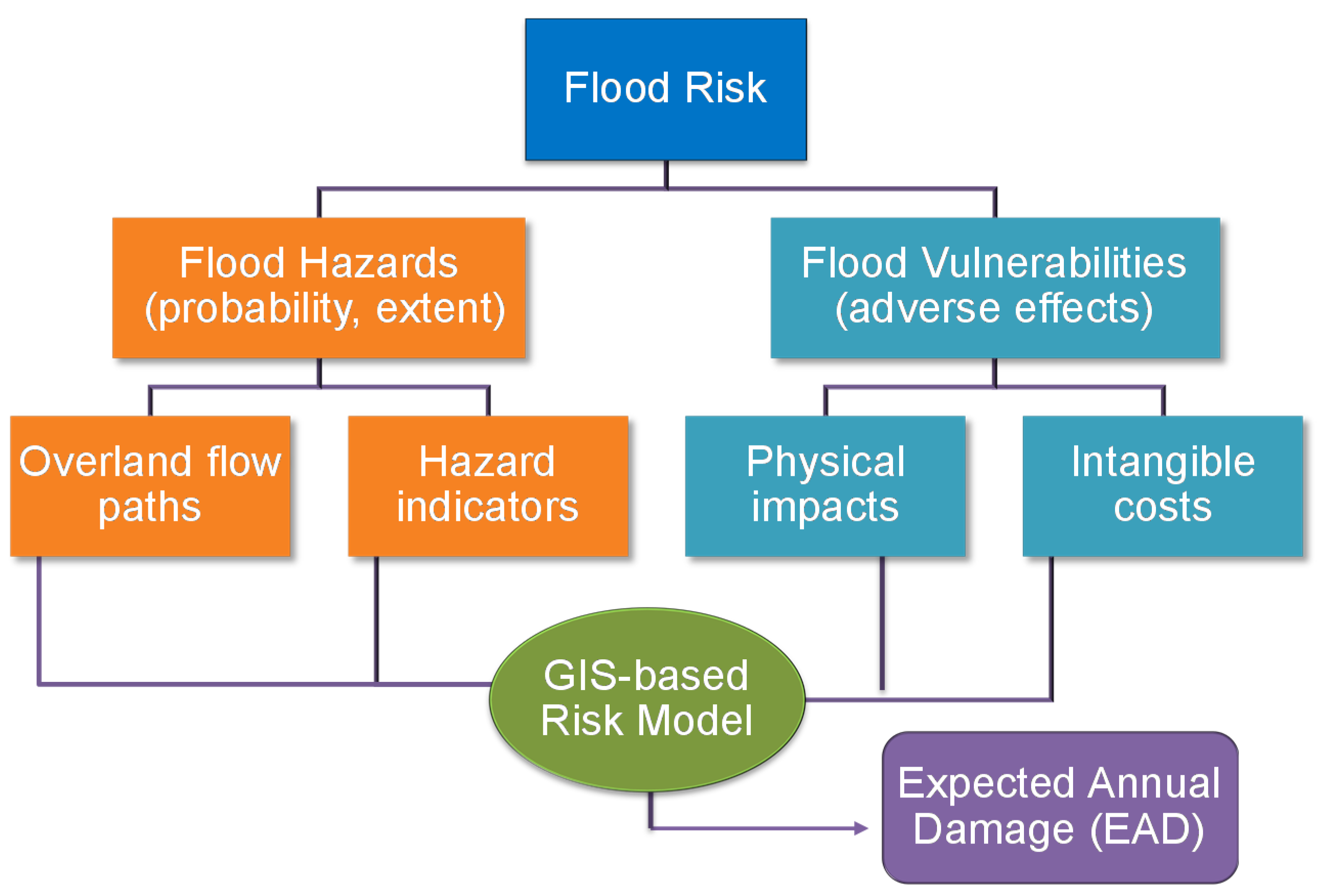
2.1. Flood Risk Assessment Framework

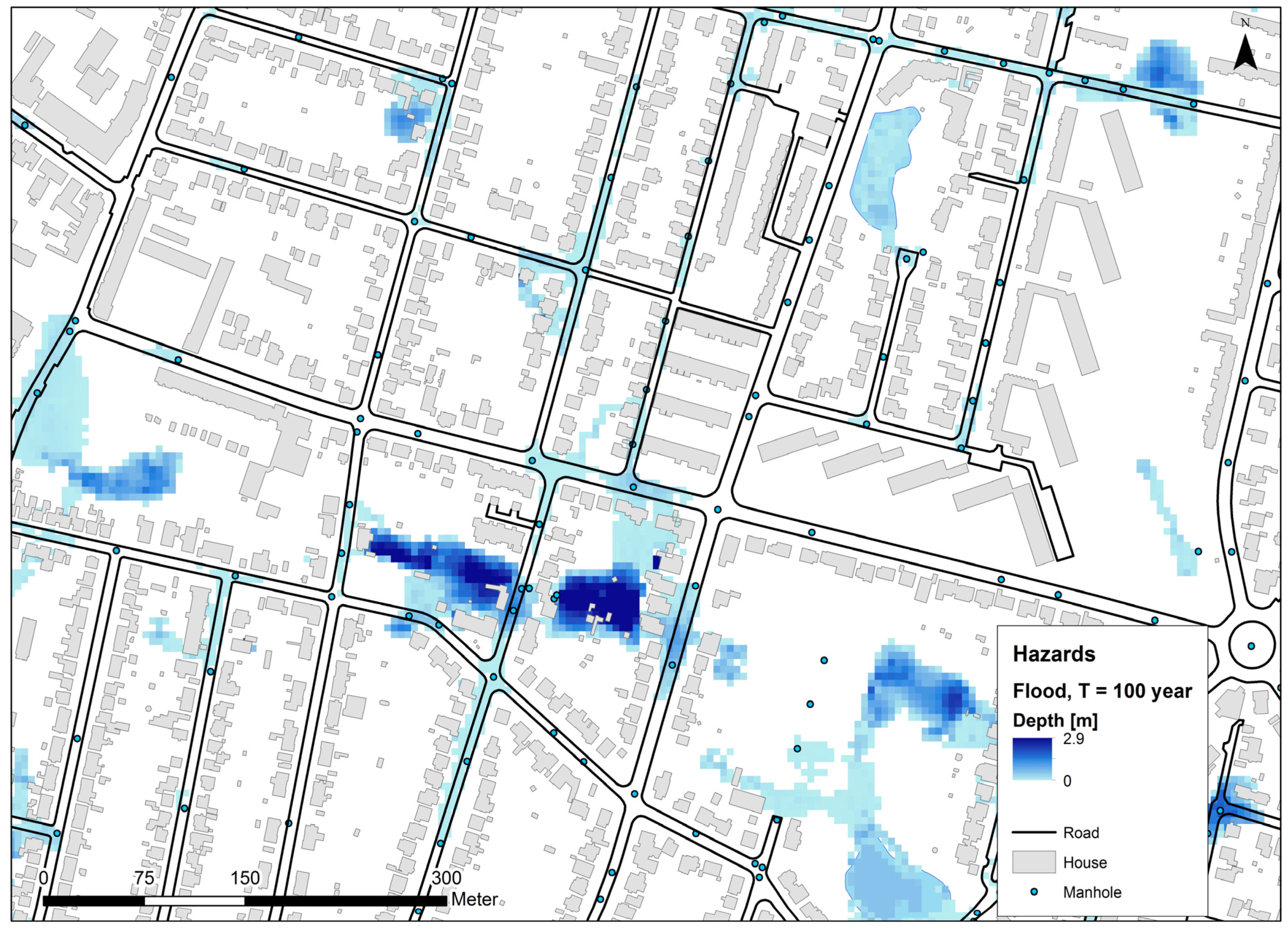
2.1.1. Flood Hazard Assessment

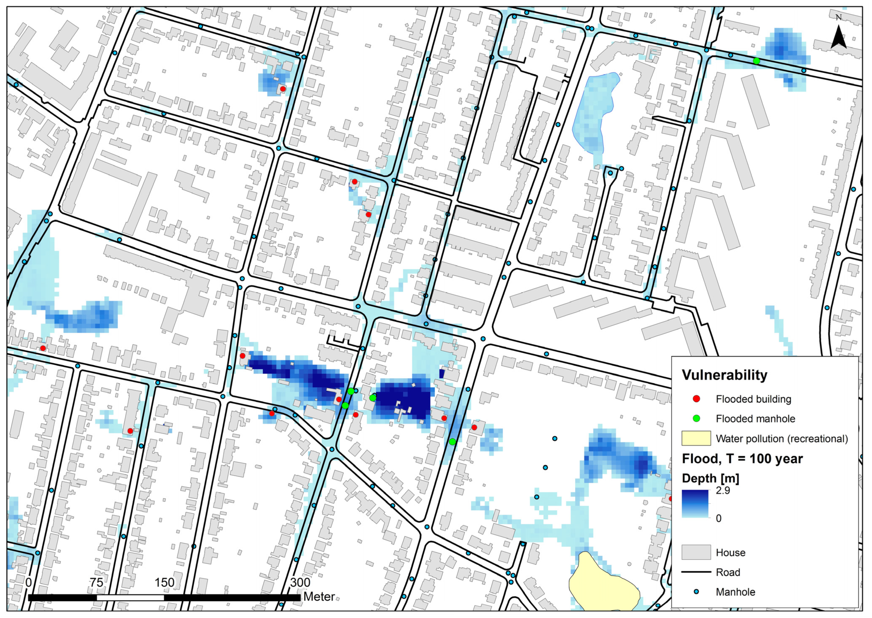
2.1.2. Vulnerability Assessment


| Damage Class | Flood Depth Threshold (m) | Unit Cost (EURO) |
|---|---|---|
| Residential | 0.10 | 13,500 |
| Commercial | 0.10 | 71,150 |
| Public Institution | 0.10 | 62,150 |
| Road | 0.30 | 6,750 |
| Manhole | 0.10 | 1,350 |
| Water pollution (recreational) | 0.15 | 67,400 |
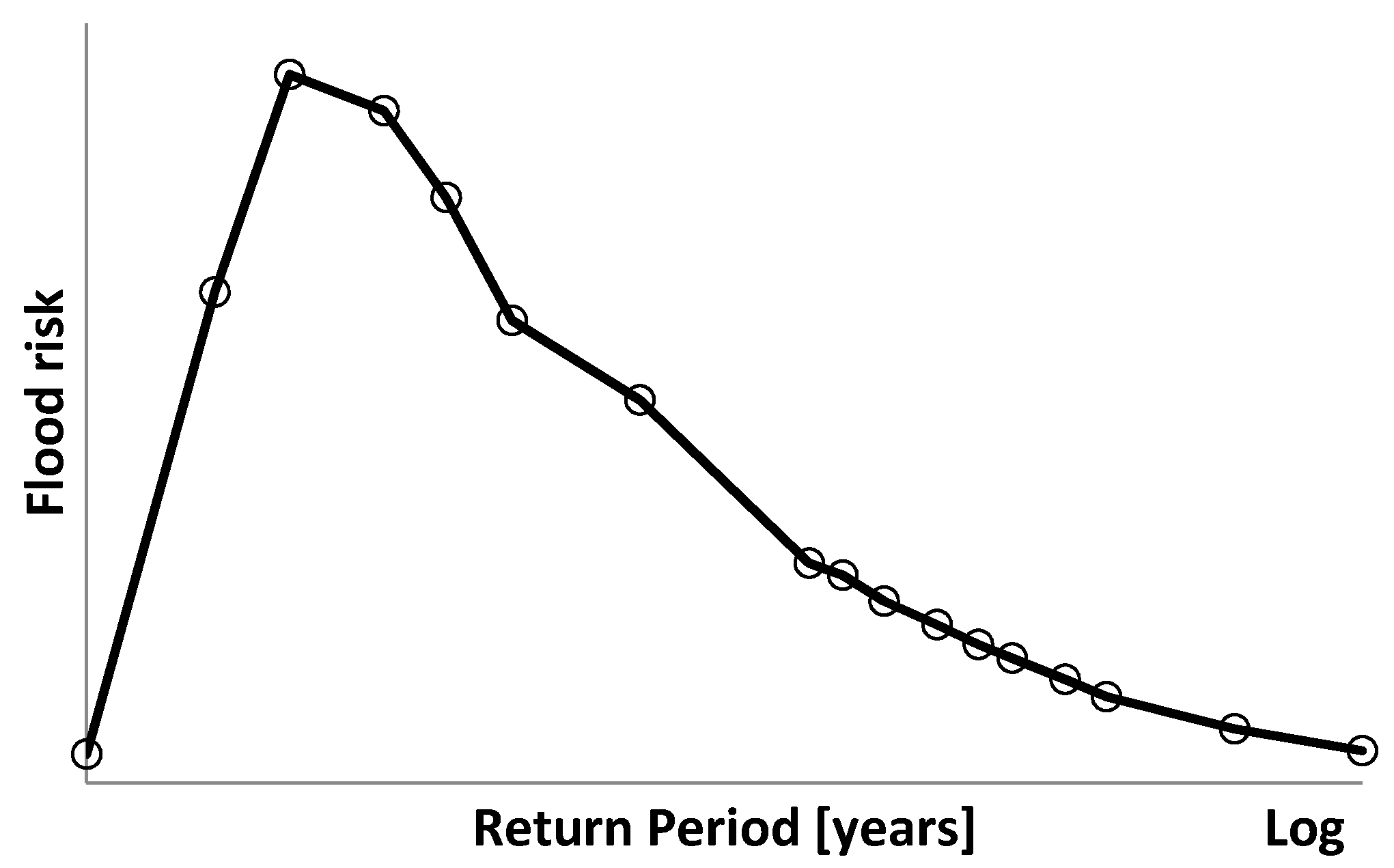
2.1.3. Risk Model


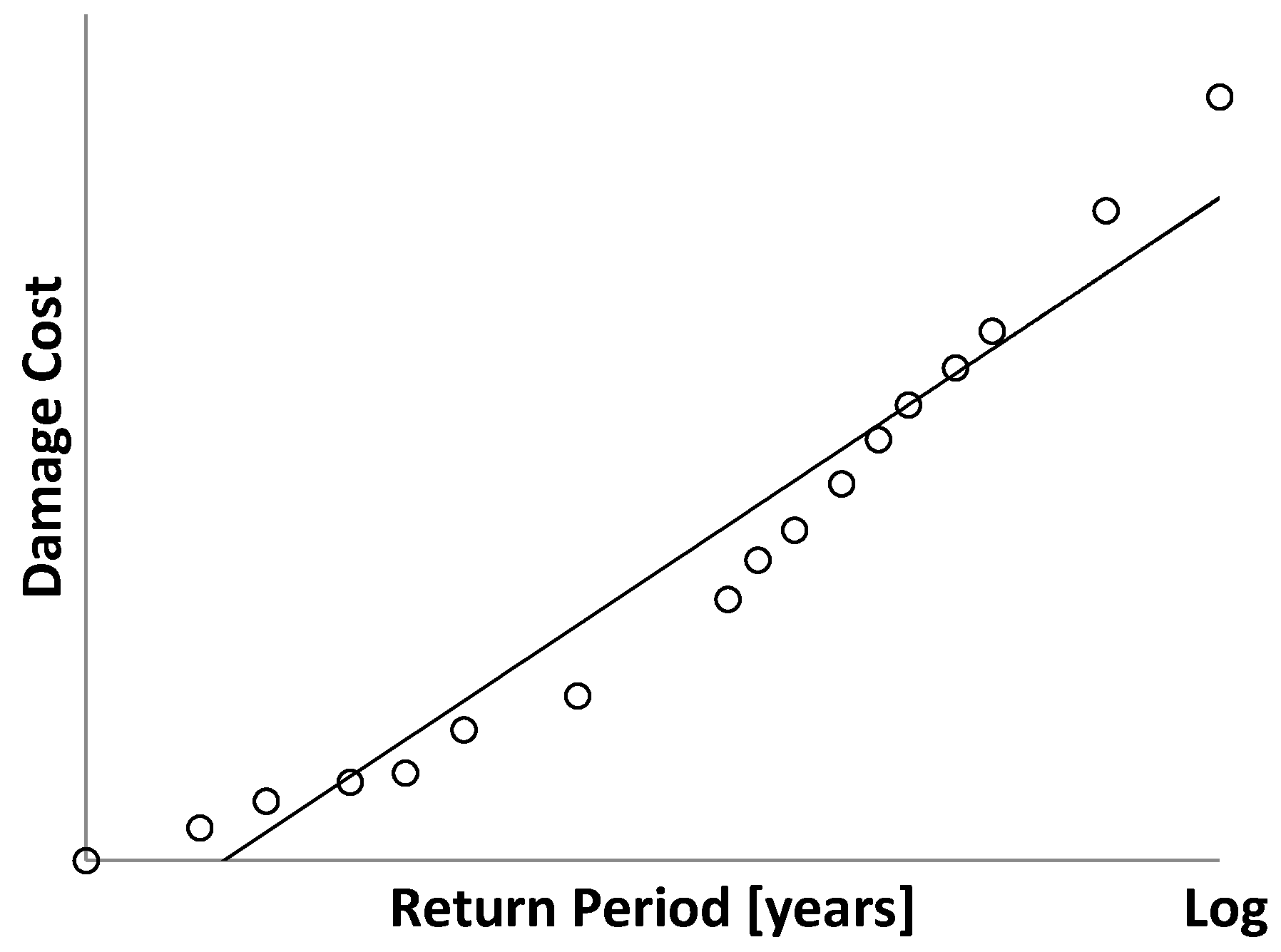
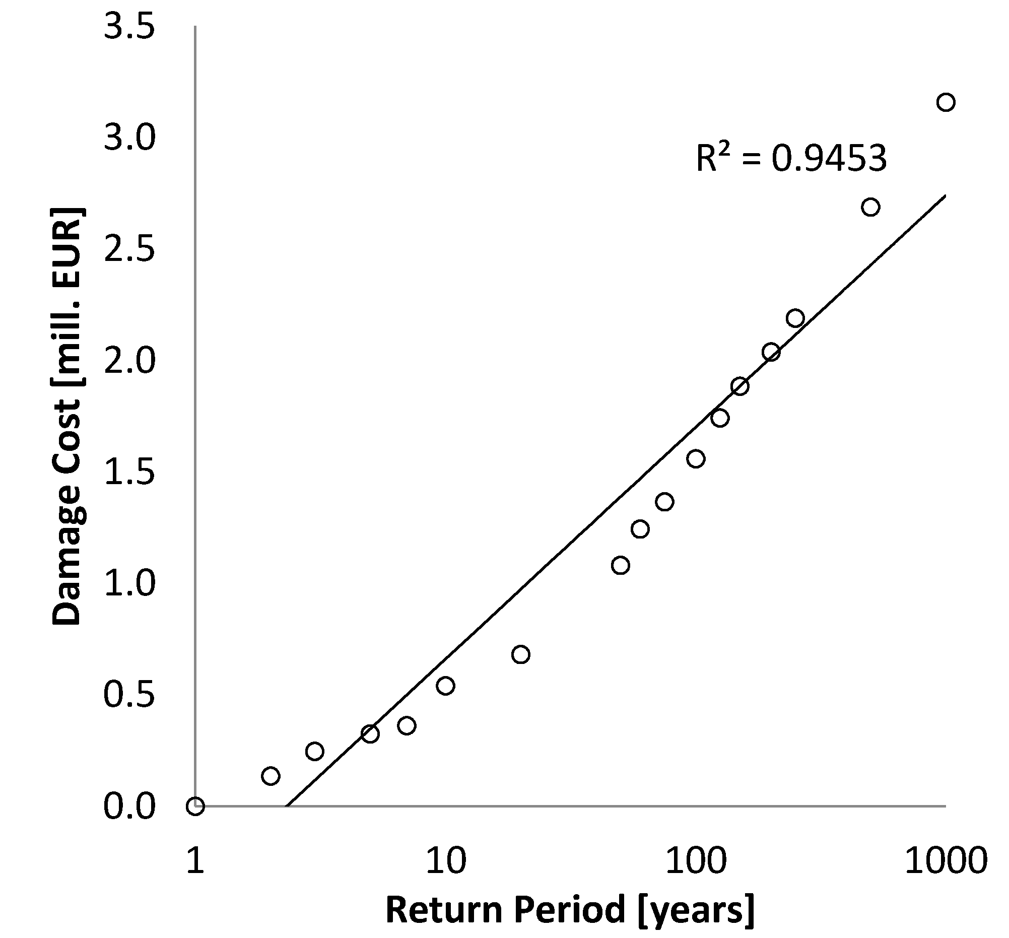
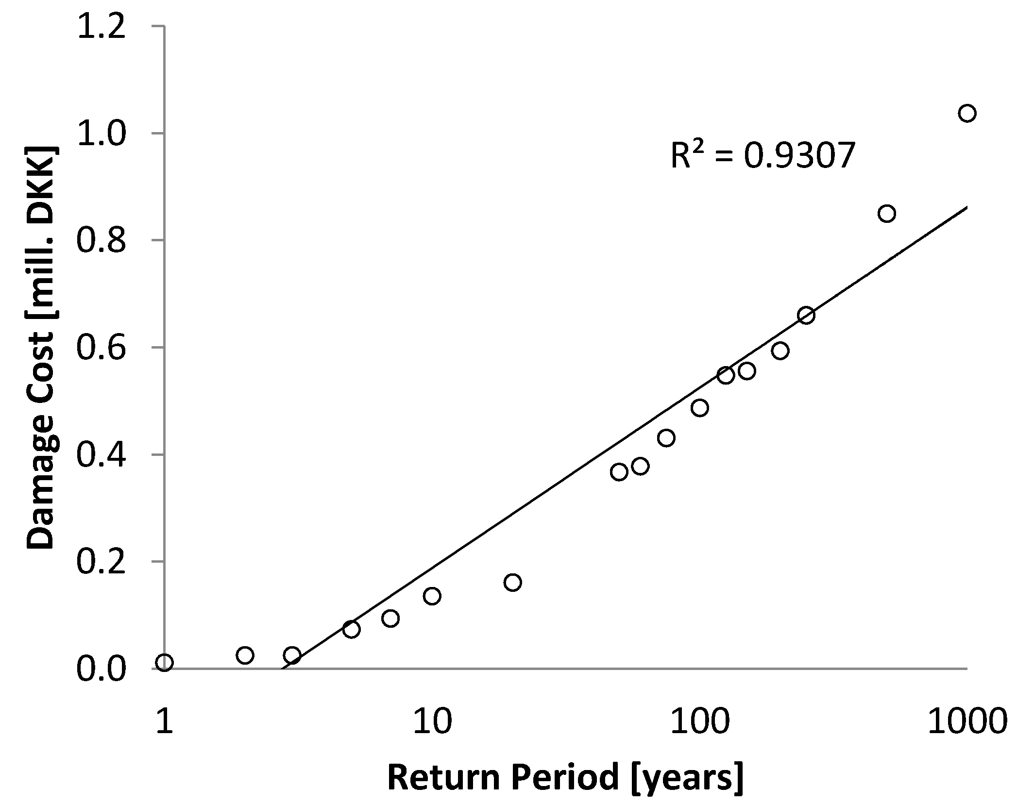
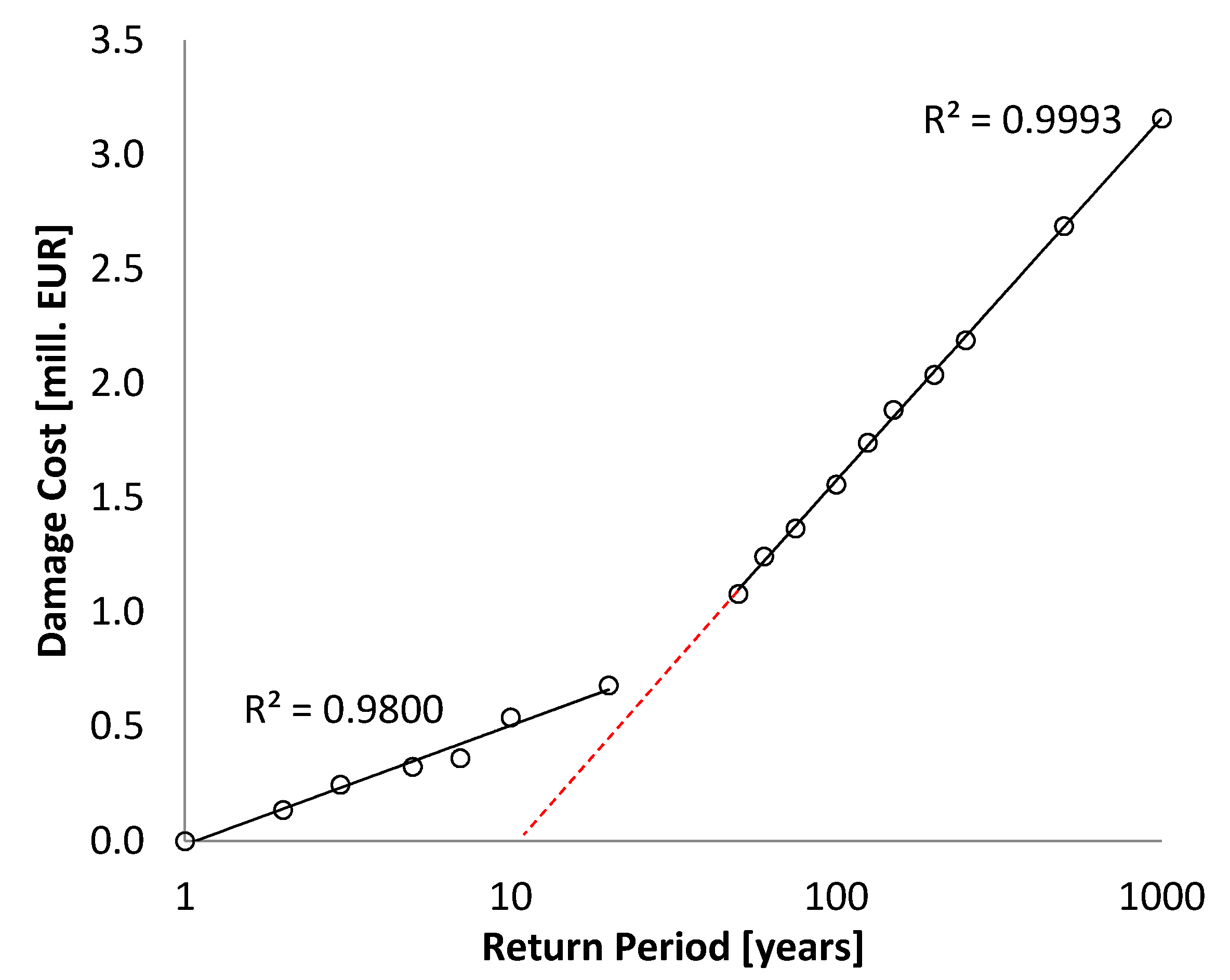
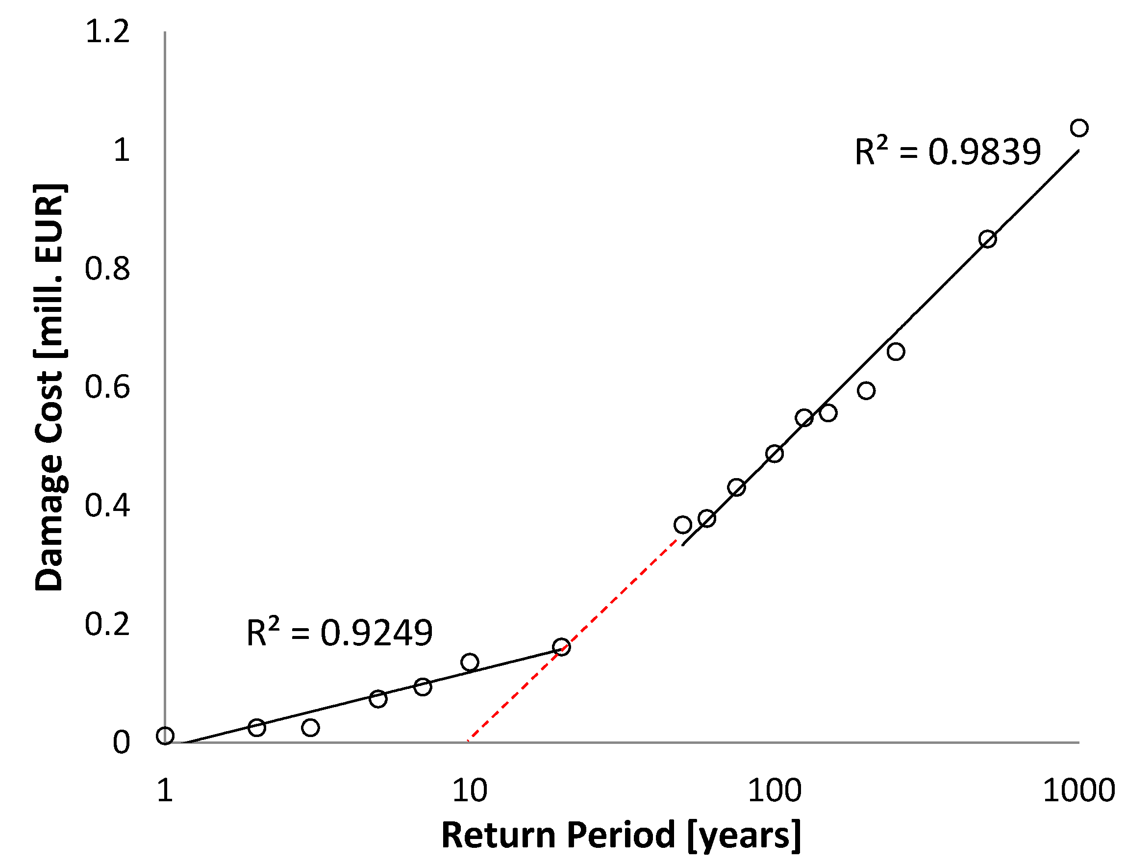
2.1.4. Expected Annual Damage (EAD)
- (a)
- Generating a Long Time Series with the Same Statistical Properties as the Damage-Cost Return Period Curve.
| Rank | Return Period | Damage Cost for Event |
|---|---|---|
| 1 | T1 | C1 |
| 2 | T2 | C2 |
| 3 | T3 | C3 |
| ··· | ··· | ··· |
| m | Tm | Cm |
| Total cost | - | |
| EAD | - | Sum/n |
- (b)
- Estimating EAD Using Numerical Integration
- (c)
- An Analytical Solution for EAD Estimation
2.2. Hypotheses to Be Tested
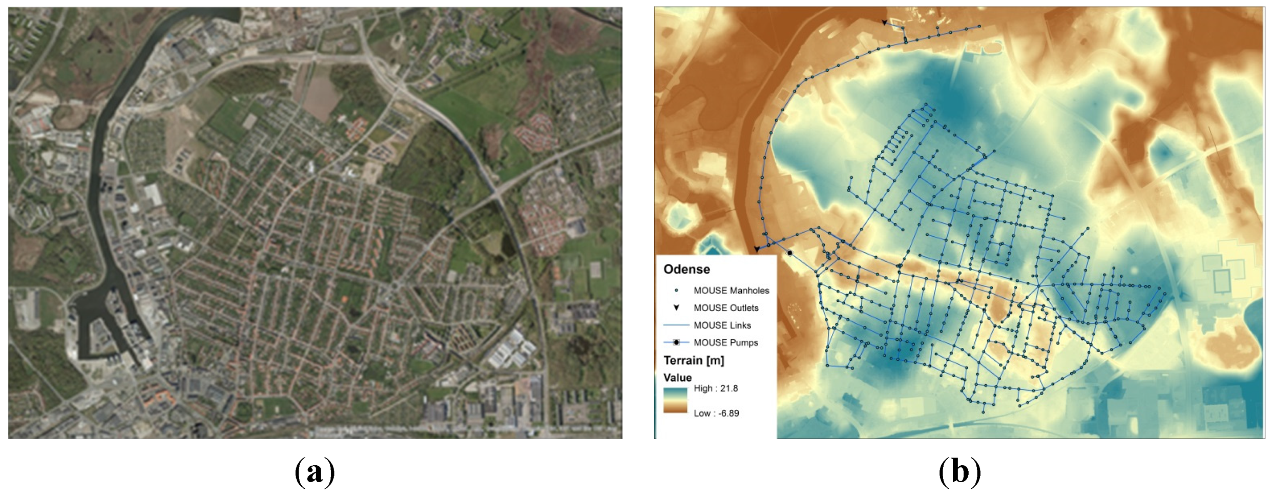
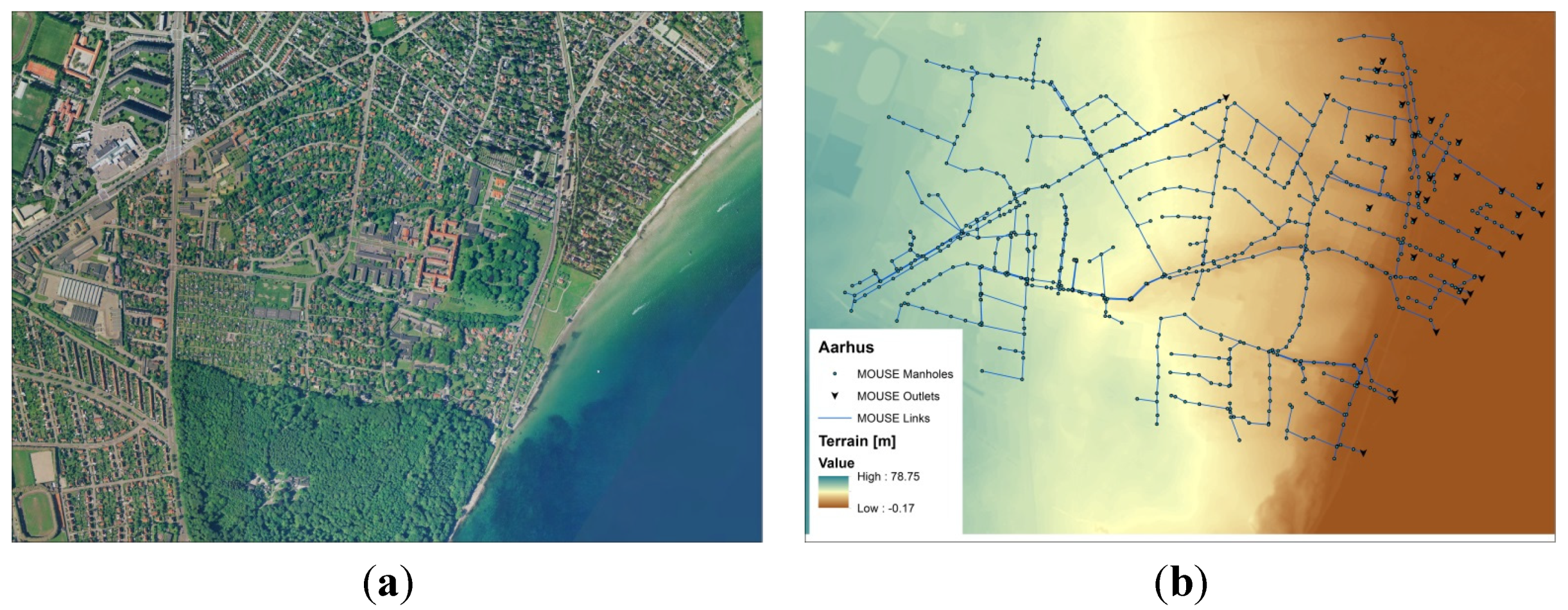
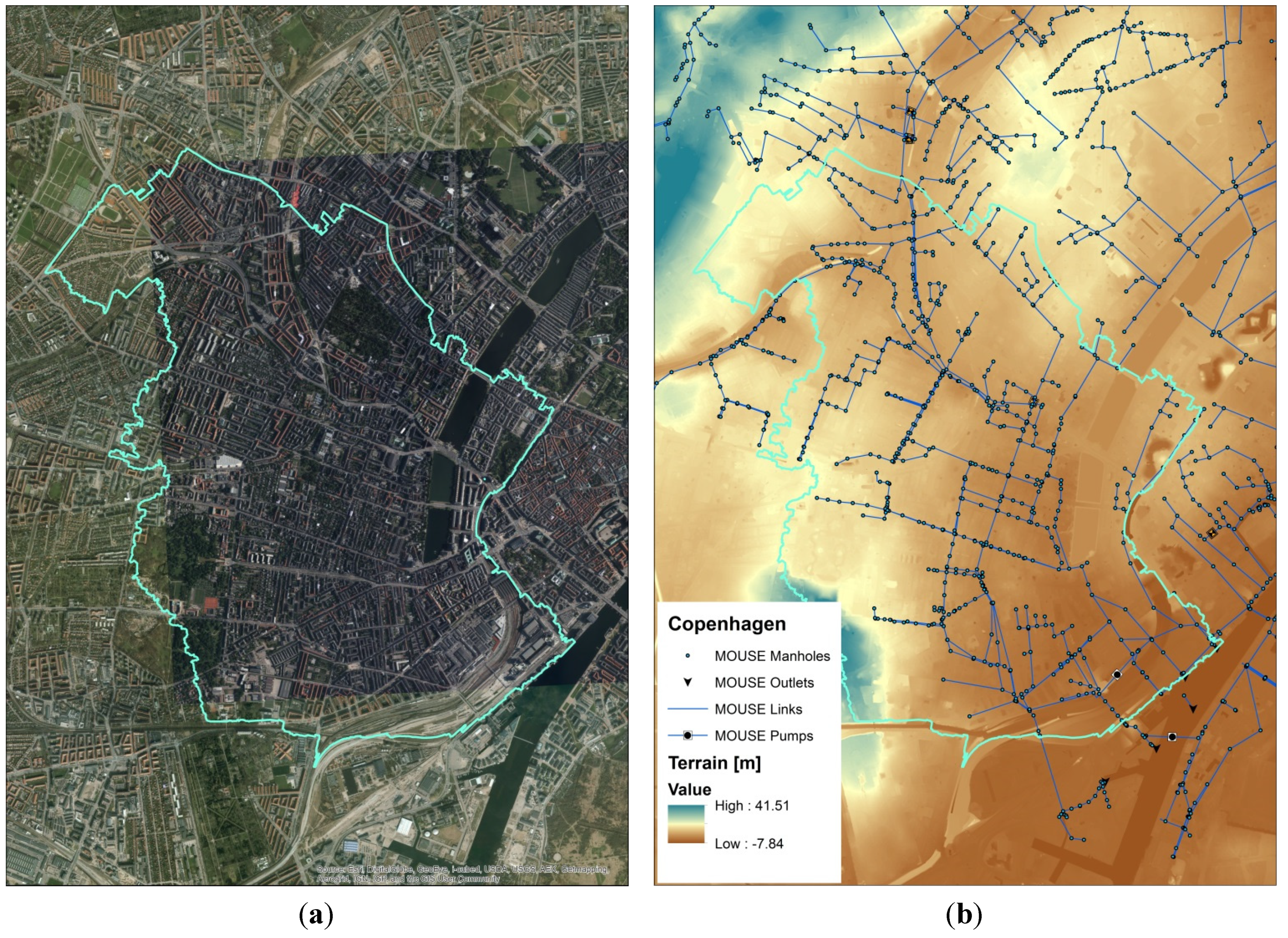
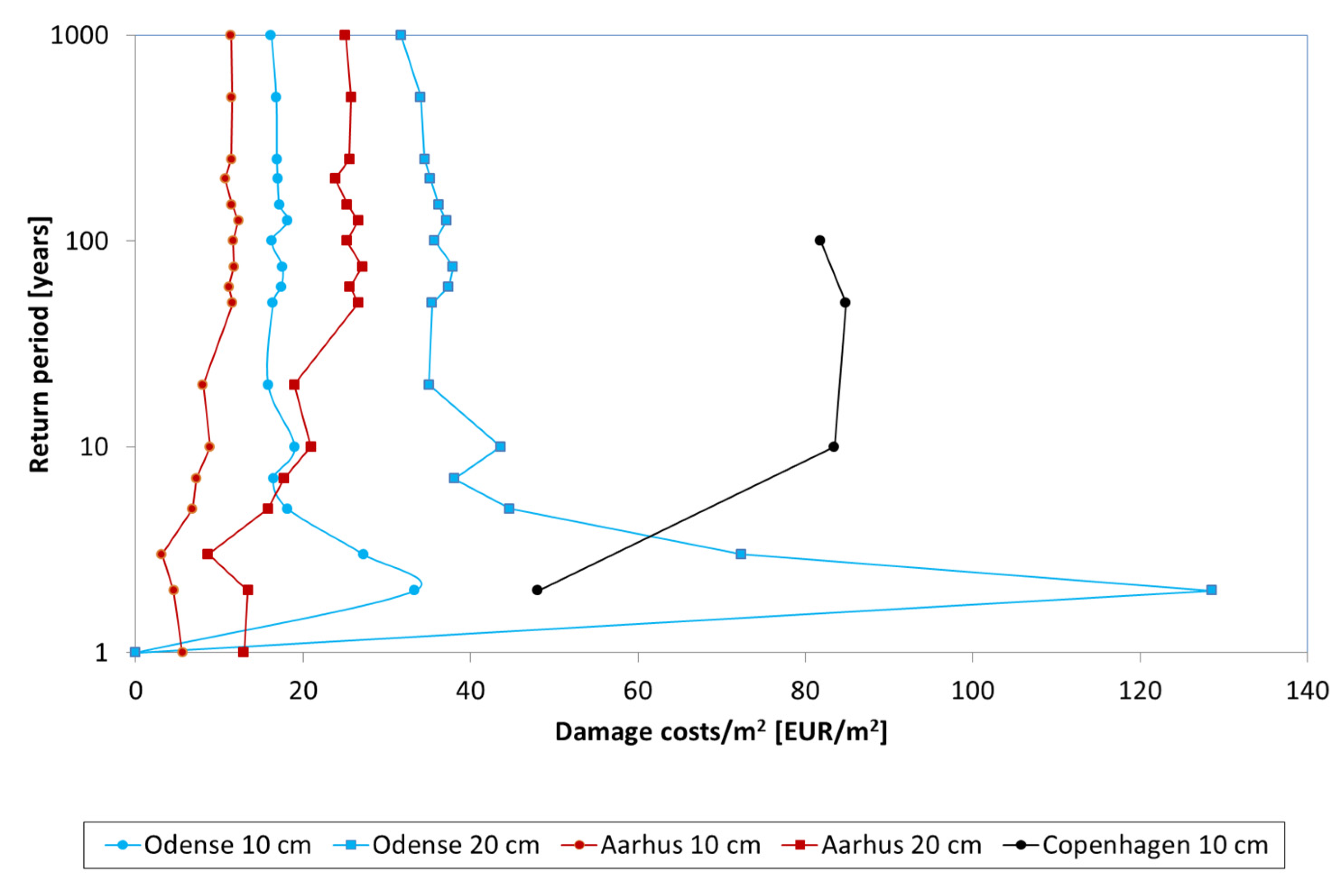
3. Study Areas


| Area | Type | Sewer System | Size (ha) | Degree of Paved Area |
|---|---|---|---|---|
| Odense (Skibhus) | Residential | Combined | 389 | 0.33 |
| Aarhus (Risskov) | Residential | Combined | 377 | 0.17 |
| Copenhagen (Nørrebro) | Residential/Commercial | Combined | 1080 | 0.55 |
4. Results and Discussion


| Method | Accounting for Log-Linear Shift | EAD [1000 EUR/Year] | |
|---|---|---|---|
| Odense | Aarhus | ||
| (a) Simulated time series | No | 189 | 51.0 |
| Yes | 220 | 52.5 | |
| (b) Numerical solution | No | 179 | 47.9 |
| Yes | 210 | 49.4 | |
| (c) Analytical solution | No | 194 | 52.8 |
| Yes | 227 | 54.7 | |
| Average | - | 203 | 51.4 |

5. Conclusions
Acknowledgments
Author Contributions
Conflicts of Interest
References
- Solomon, S.; Qin, D.; Manning, M.; Marquis, M.; Averyt, K.; Tignor, M.B.M.; Miller, H.L., Jr.; Chen, Z. Climate Change 2007: The Physical Science Basis; Cambridge University Press: Cambridge, UK, 2007. [Google Scholar]
- Madsen, H.; Arnbjerg-Nielsen, K.; Mikkelsen, P.S. Update of regional intensity-duration-frequency curves in Denmark: Tendency towards increased storm intensities. Atmos. Res. 2009, 92, 343–349. [Google Scholar] [CrossRef]
- Arnbjerg-Nielsen, K. Past, present and future design of urban drainage systems with focus on Danish experiences. Water Sci. Technol. 2011, 63, 527–535. [Google Scholar] [CrossRef] [PubMed]
- Freni, G.; la Loggia, G.; Notaro, V. Uncertainty in urban flood damage assessment due to urban drainage modeling and depth-damage curve estimation. Water Sci. Technol. 2010, 61, 2979–2993. [Google Scholar] [CrossRef] [PubMed]
- Ashley, R.; Garvin, S.; Pasche, E.; Vassilopoulos, A.; Zevenbergen, C. Advances in Urban Flood Management; Taylor & Francis Group: London, UK, 2007. [Google Scholar]
- Zhou, Q.; Mikkelsen, P.M.; Halsnæs, K.; Arnbjerg-Nielsen, K. Framework for economic pluvial flood risk assessment considering climate change effects and adaptation benefits. J. Hydrol. 2012, 414–415, 539–549. [Google Scholar] [CrossRef]
- Schneider, S.H.; Semenov, S.; Patwardhan, A.; Burton, I.; Magadza, C.H.D.; Oppenheimer, M.; Pittock, A.B.; Rahman, A.; Smith, J.B.; Suarez, A.; Yamin, F. Assessing key vulnerabilities and the risk from climate change. In Climate Change 2007: Impacts, Adaptation and Vulnerability. Contribution of Working Group II to the Fourth Assessment Report of the Intergovernmental Panel on Climate Change; Parry, M.L., Canziani, O.F., Palutikof, J.P., van der Linden, P.J., Hanson, C.E., Eds.; Cambridge University Press: Cambridge, UK, 2007; pp. 779–810. [Google Scholar]
- MOUSE Surface Runoff Models Reference Manual; DHI: Hørsholm, Denmark, 2002.
- MIKE FLOOD 1D-2D Modeling, User Manual; DHI: Hørsholm, Denmark, 2011.
- Hede, M.; Kolby, T. Evaluation of Flood Risk Assessment and Climate Change Adaptation Measures in Copenhagen. Master Thesis, Department of Environmental Engineering, Technical University of Denmark, Lyngby, Denmark, 2013. [Google Scholar]
- Fontanazza, C.M.; Freni, G.; la Loggia, G.; Notaro, V. Uncertainty evaluation of design rainfall for urban flood risk analysis. Water Sci. Technol. 2011, 63, 2641–2650. [Google Scholar] [CrossRef] [PubMed]
- Ten Veldhuis, J.A.E.; Clemens, F.H.L.R. Flood risk modeling based on tangible and intangible urban flood damage quantification. Water Sci. Technol. 2010, 62, 189–195. [Google Scholar] [CrossRef] [PubMed]
- De Moel, H.; Aerts, J.C.H. Effect of uncertainty in land use, damage models and inundation depth on flood damage estimates. Nat. Hazards 2011, 58, 407–425. [Google Scholar] [CrossRef]
- Apel, H.; Thieken, A.H.; Merz, B.; Blöschl, G. Flood risk assessment and associated uncertainty. Nat. Hazards Earth Syst. Sci. 2004, 4, 295–308. [Google Scholar] [CrossRef]
- Ballesteros-Canovas, J.A.; Sanchez-Silva, M.; Bodoque, J.M.; Diez-Herrero, A. An integrated approach to flood risk management: A case study of Navaluenga (Central Spain). Water Resour. Manag. 2013, 27, 3051–3069. [Google Scholar] [CrossRef]
- Arnbjerg-Nielsen, K.; Fleischer, H.S. Feasible adaptation strategies for increased risk of flooding in cities due to climate change. Water Sci. Technol. 2009, 60, 273–281. [Google Scholar] [CrossRef] [PubMed]
- Institut for Beredskabsevaluering. Redegørelse vedrørende skybruddet i Storkøbenhavn lørdag den 2. juli 2011. Available online: http://brs.dk/beredskab/Documents/Redeg%C3%B8relse%20om%20skybruddet%20i%20Stork%C3%B8benhavn%202.%20juli%202011.pdf (accessed on 19 July 2013). (In Danish)
- Ward, P.J.; de Moel, H.; Aerts, J.C.J.H. How are flood risk estimates affected by the choice of return-periods? Nat. Hazards Earth Syst. Sci. 2011, 11, 3181–3195. [Google Scholar] [CrossRef]
- Chow, V.T.; Maidment, D.R.; Mays, L.W. Applied Hydrology; McGraw-Hill: New York, NY, USA, 1988. [Google Scholar]
- Rosbjerg, D. A Defense of the Median Plotting Position; Progress Report No. 66; Institute of Hydrodynamics and Hydraulic Engineering, Technical University of Denmark: Lyngby, Denmark, 1988; pp. 17–28. [Google Scholar]
- IDA Spildevandkomiteen (The Water Pollution Committee of the Society of Danish Engineers). Skrift nr. 27: Funktionspraksis for Afløbssystemer Under Regn 2005. Available online: http://ida.dk/sites/prod.ida.dk/files/Skrift27Funktionspraksisforafl%C3%B8bssystemerunderregn.pdf (accessed on 24 April 2013). (In Danish)
- Merz, B.; Kreibich, H.; Schwarze, R.; Thieken, A. Assessment of economic flood damage. Nat. Hazards Earth Syst. Sci. 2010, 10, 1697–1724. [Google Scholar] [CrossRef]
© 2015 by the authors; licensee MDPI, Basel, Switzerland. This article is an open access article distributed under the terms and conditions of the Creative Commons Attribution license (http://creativecommons.org/licenses/by/4.0/).
Share and Cite
Olsen, A.S.; Zhou, Q.; Linde, J.J.; Arnbjerg-Nielsen, K. Comparing Methods of Calculating Expected Annual Damage in Urban Pluvial Flood Risk Assessments. Water 2015, 7, 255-270. https://doi.org/10.3390/w7010255
Olsen AS, Zhou Q, Linde JJ, Arnbjerg-Nielsen K. Comparing Methods of Calculating Expected Annual Damage in Urban Pluvial Flood Risk Assessments. Water. 2015; 7(1):255-270. https://doi.org/10.3390/w7010255
Chicago/Turabian StyleOlsen, Anders Skovgård, Qianqian Zhou, Jens Jørgen Linde, and Karsten Arnbjerg-Nielsen. 2015. "Comparing Methods of Calculating Expected Annual Damage in Urban Pluvial Flood Risk Assessments" Water 7, no. 1: 255-270. https://doi.org/10.3390/w7010255