
Discharge Alterations of the Mures River, Romania under Ensembles of Future Climate Projections and Sequential Threats to Aquatic Ecosystem by the End of the Century

Abstract
:1. Introduction
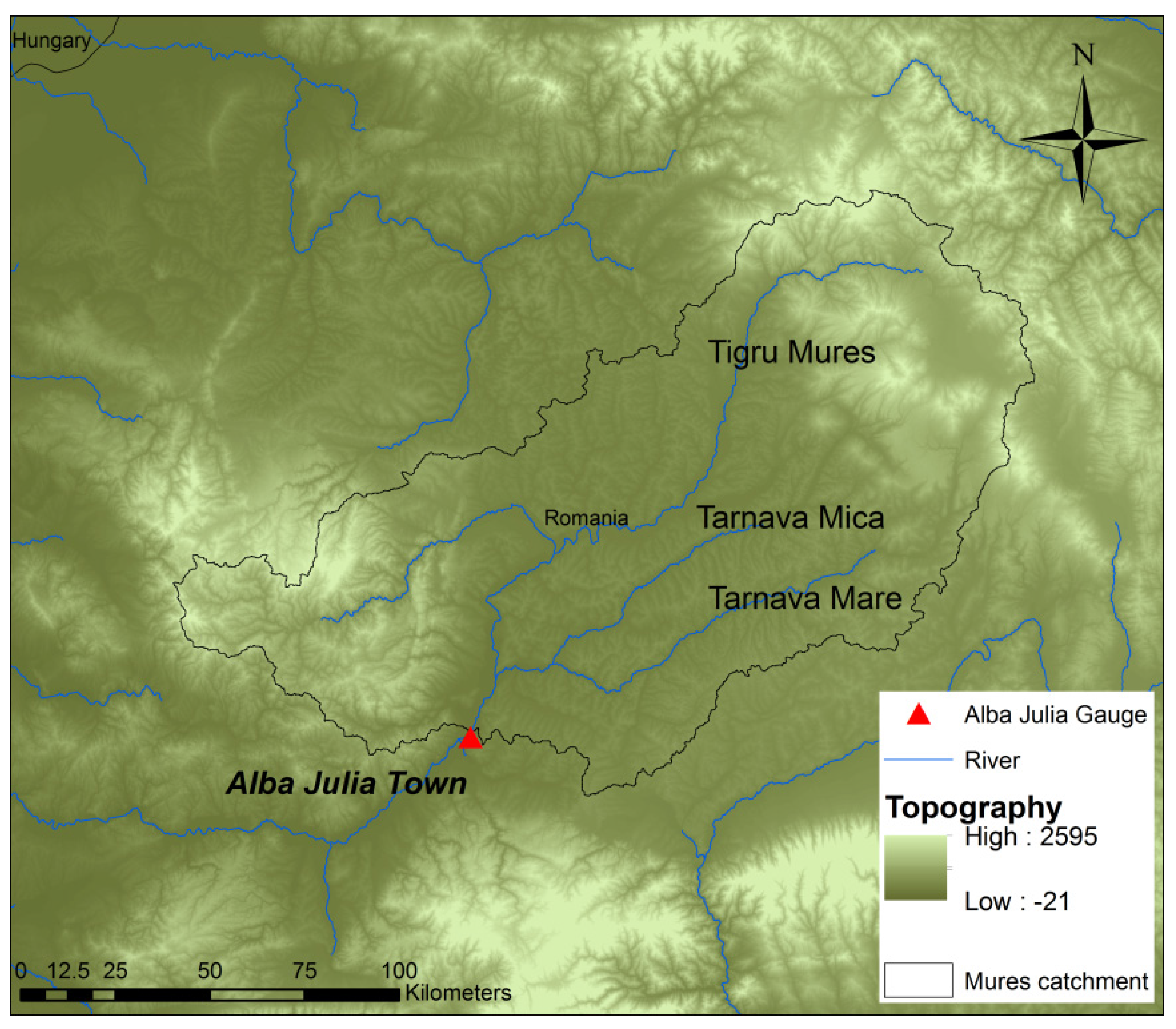
2. Study Area

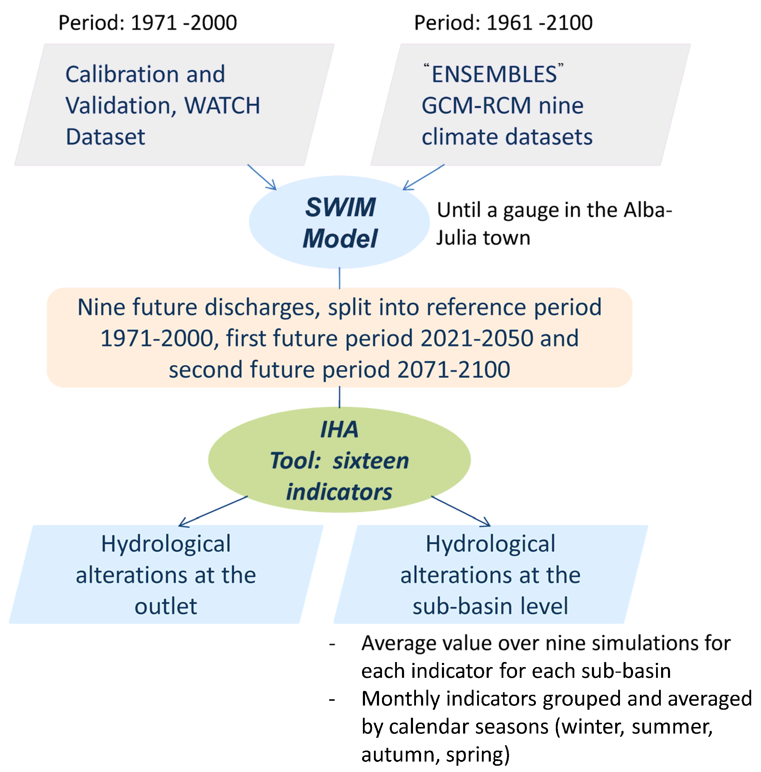
3. Methods

3.1. SWIM Model Description
3.2. IHA Method

| IHA Group | Hydrological Parameters | Functional Link to the Aquatic Ecosystem |
|---|---|---|
| Magnitude of monthly water conditions | Median monthly discharge (twelve indicators) | Provide adequate habitat area; Maintain water temperature, dissolved oxygen; Drinking water for terrestrial animals; Groundwater tables, soil moisture |
| Timing of annual extremes | Average duration of low pulse event (below 25 percentile) Average duration of high pulse event (exceeding 75 percentile) No. of high pulses each year No. of low pulses each year | Induced velocities, sediment transport and erosion; Water temperature; Connection to flood plains Water availability for habitat area; Ensure migration and spawning paths for fishes Trigger new life-cycles; Provide floodplains with nutrients, ensure connection of floodplain with main channel |
| Total | 16 Indicators | - |
3.3. Data
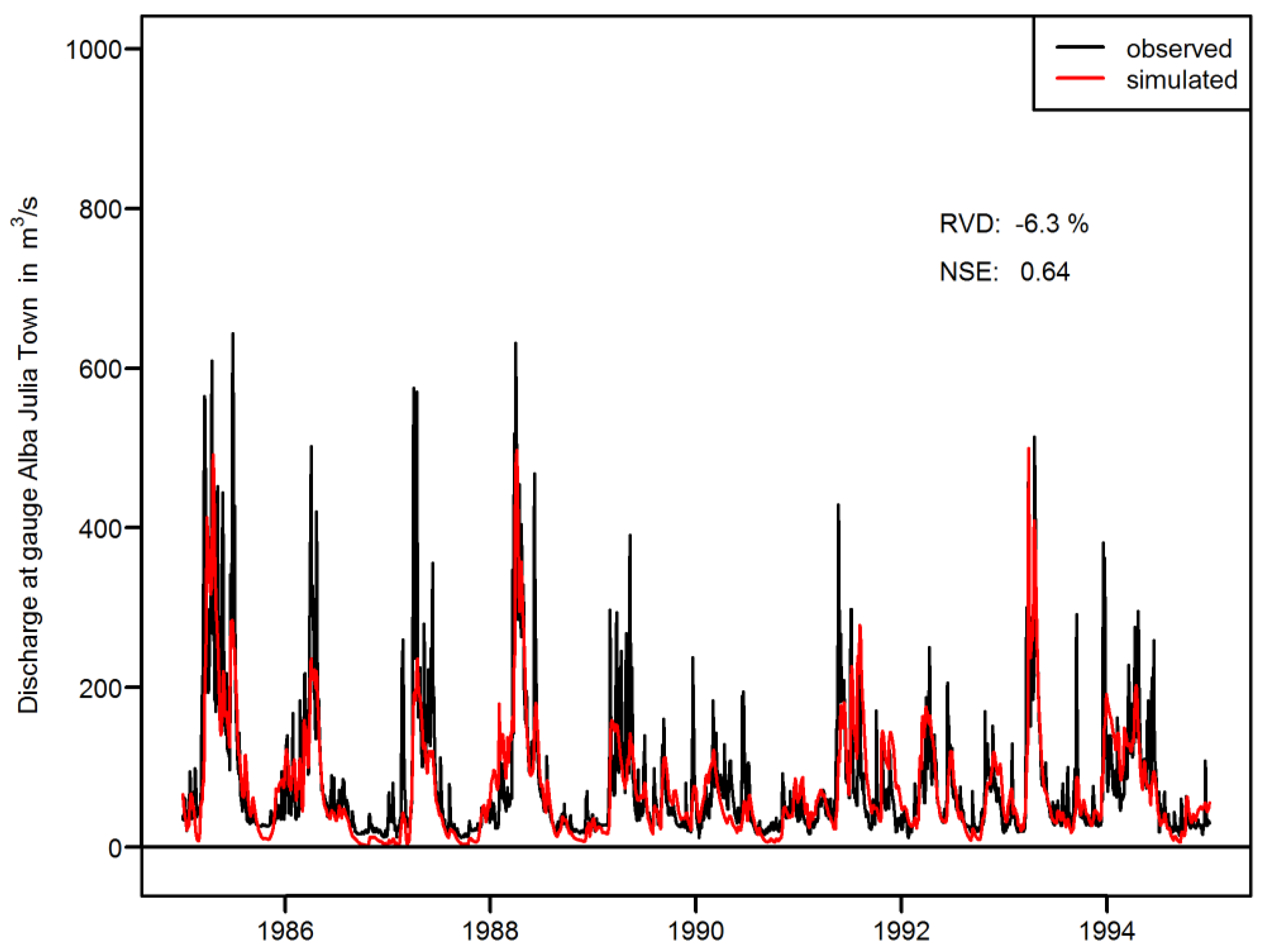
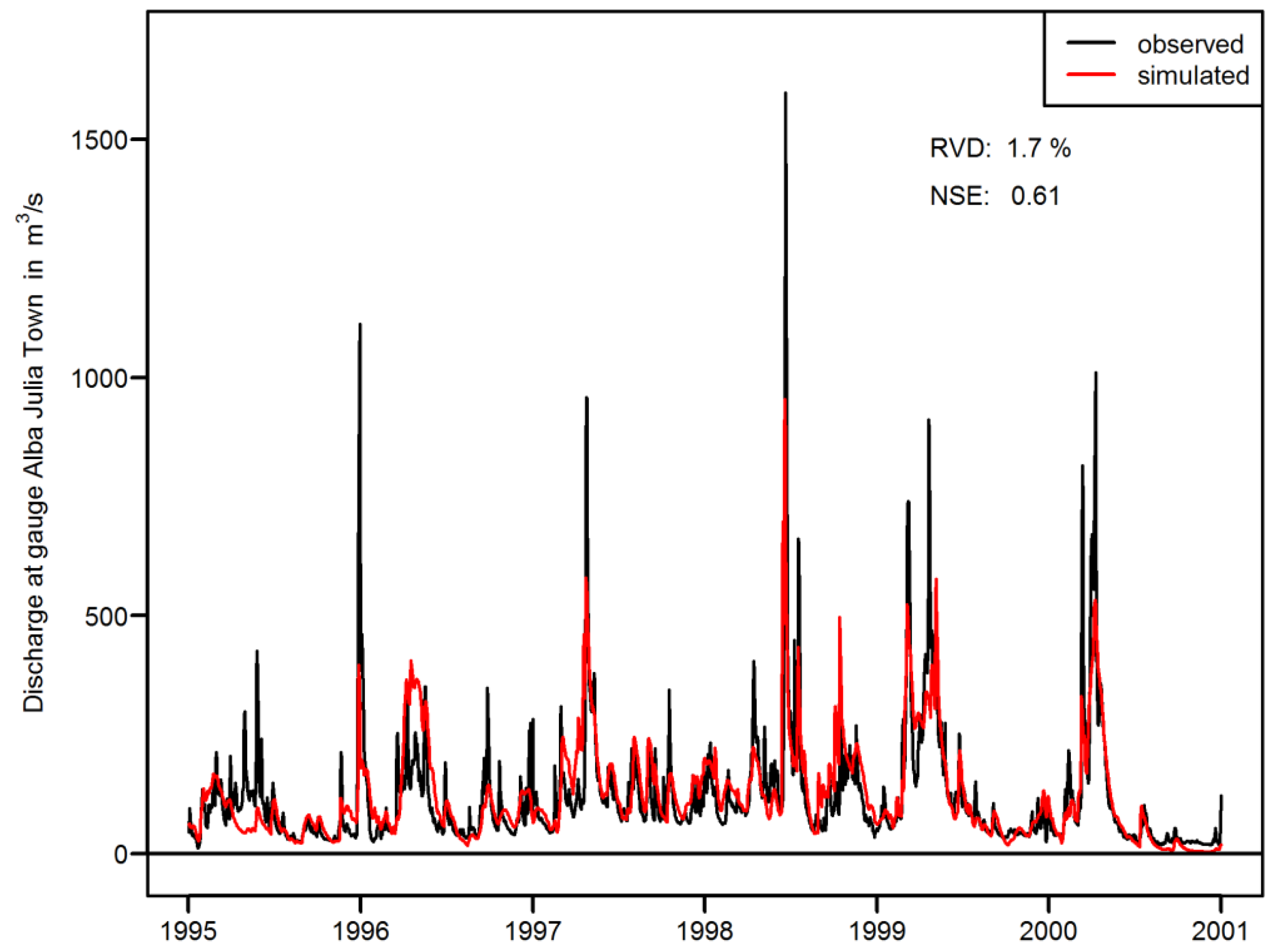
3.4. Model Calibration and Validation
3.5. Climate Scenarios
| RCM | GCM | Name Used in This Study | ||
|---|---|---|---|---|
| MPIMET | NERSC | CNRM | ||
| DMI | x | DMI | ||
| DMI | x | DMI-NERSC | ||
| DMI | x | DMI-CNRM | ||
| HadRM | x | HadRM | ||
| ICTP | x | ICTP | ||
| KMNI | x | KMNI | ||
| MPI | x | MPI | ||
| SMHI | x | SMHI | ||
| SMHI | x | SMHI-NERSC | ||
4. Results and Discussion
4.1. Model Performance


4.2. Future Climate Projections in the Context of Hydrological Modeling
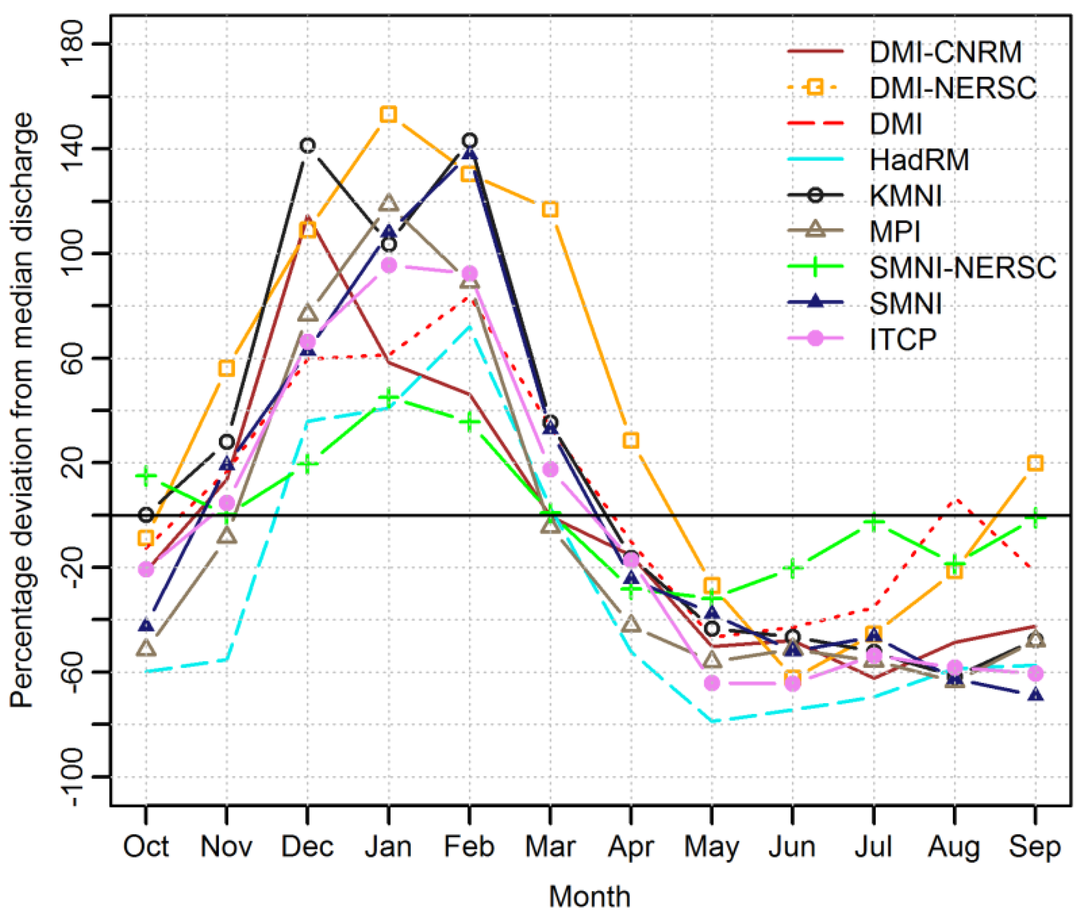
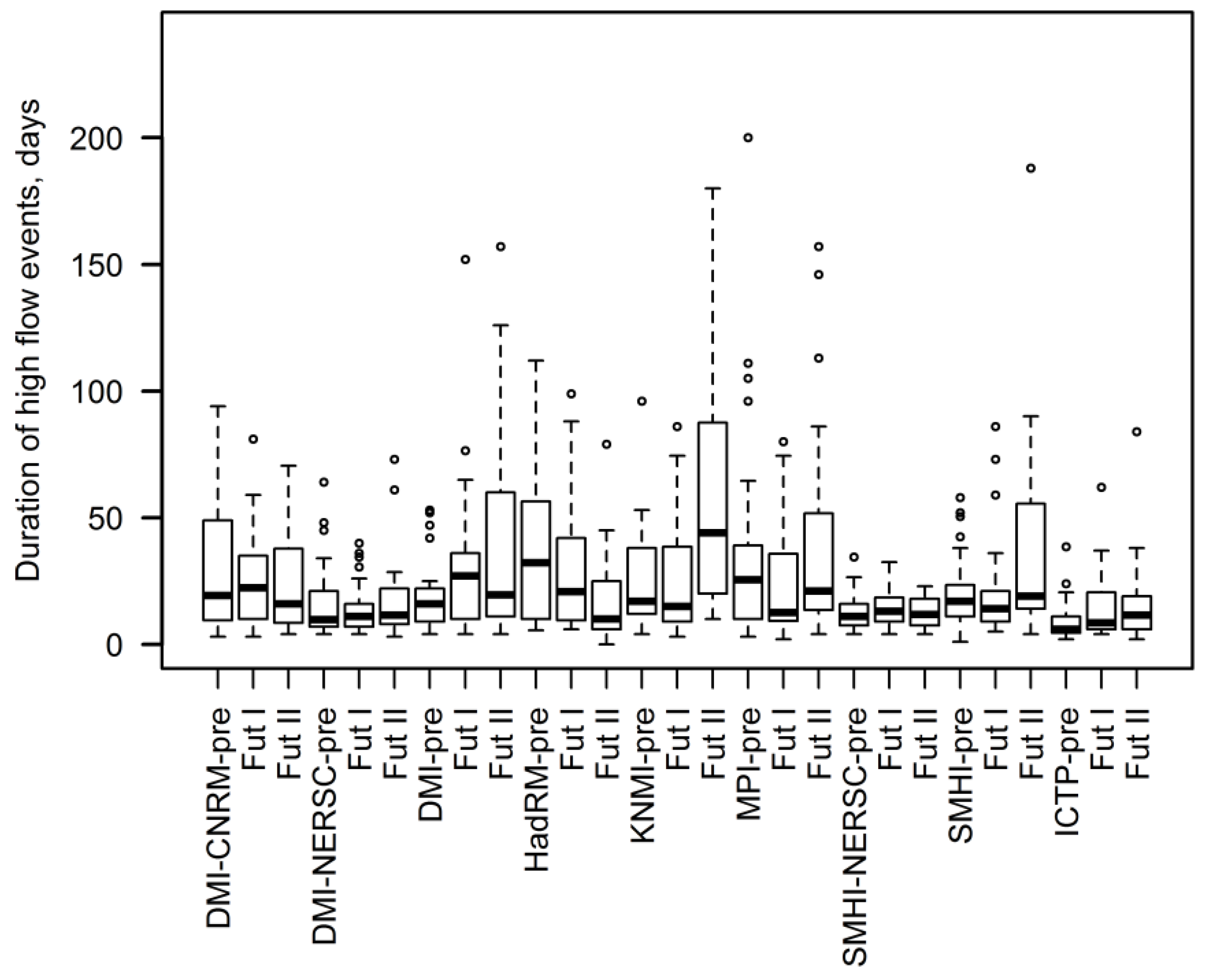
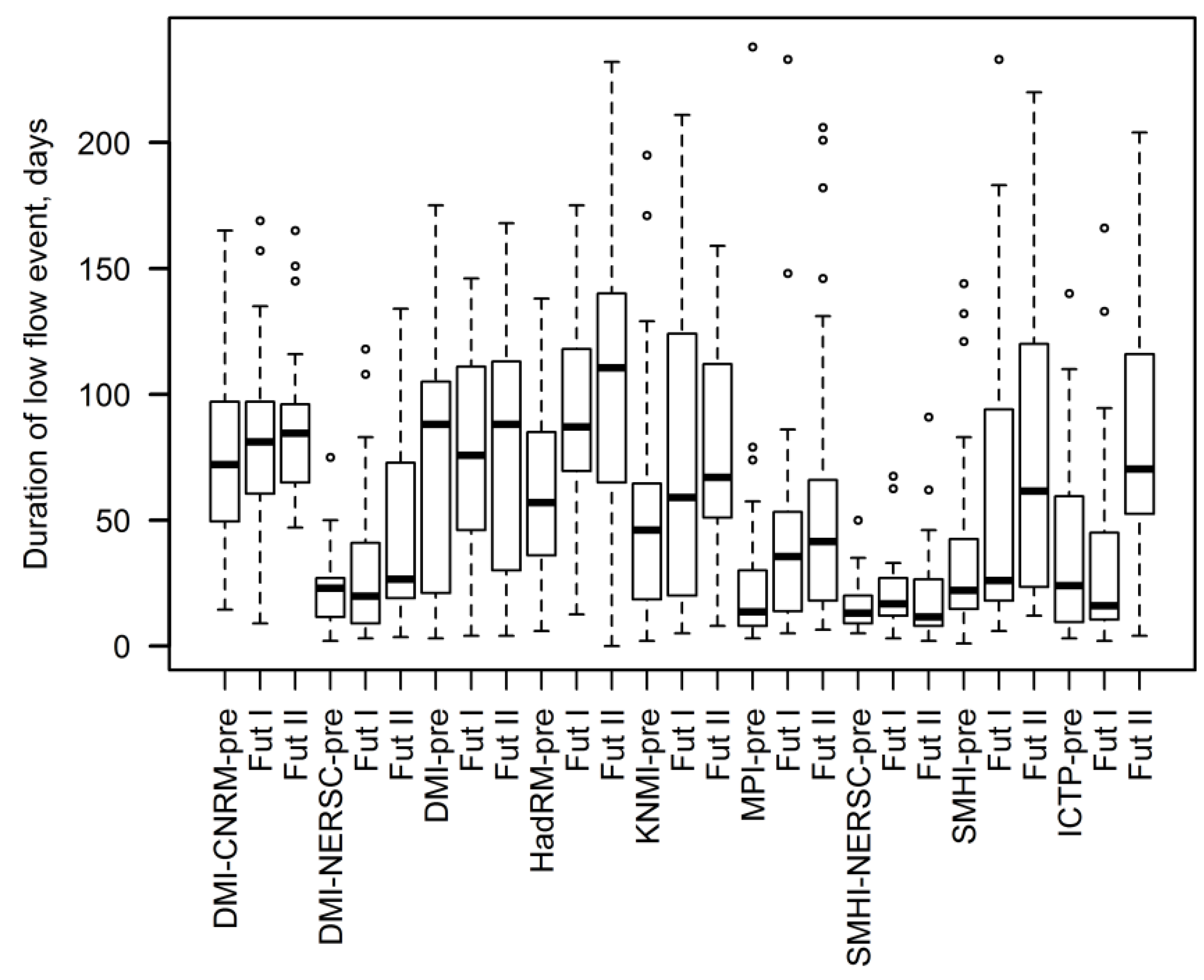
4.3. IHA Analysis for Monthly Median Discharge, High and Low Flow Events Alterations


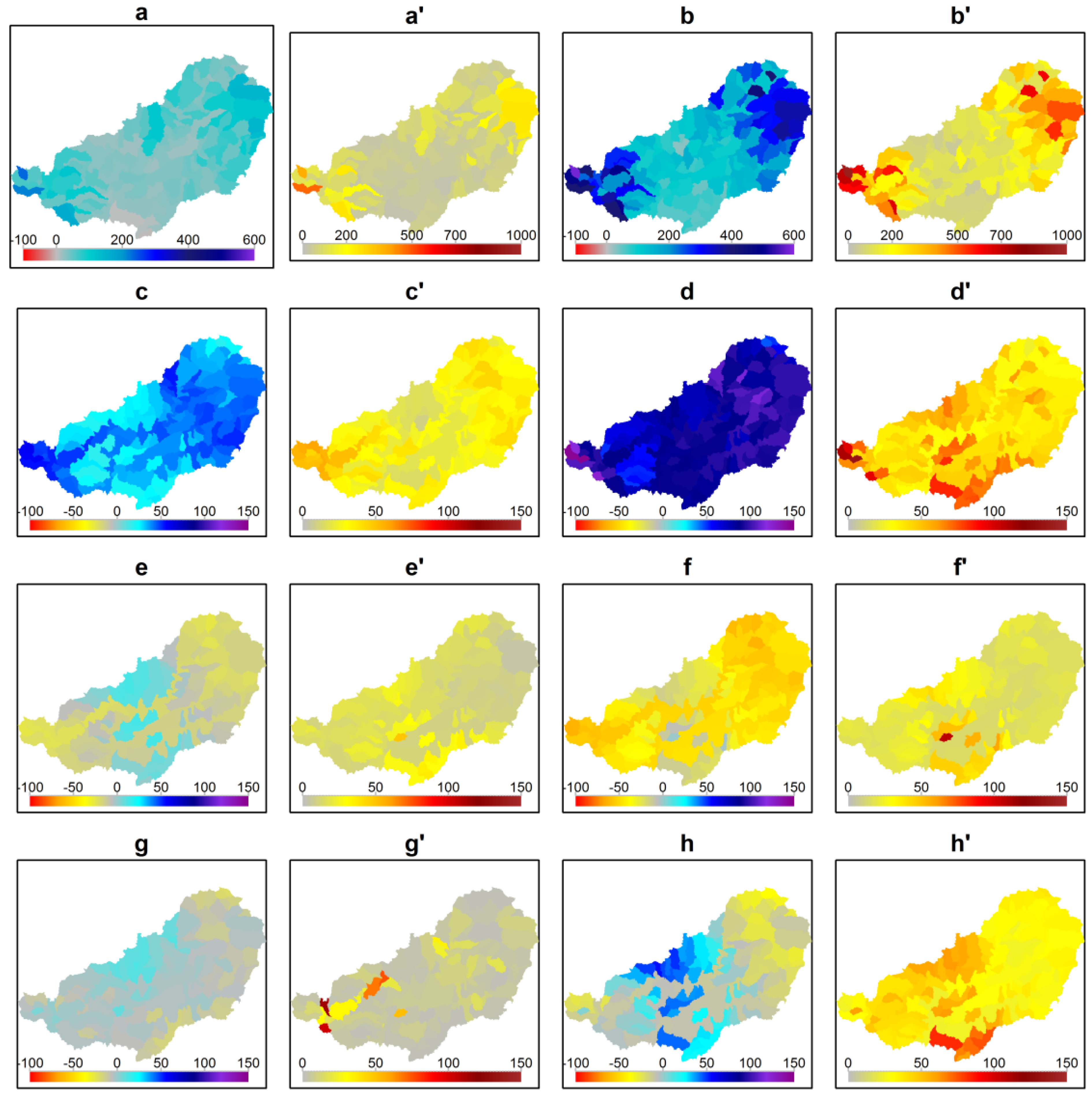
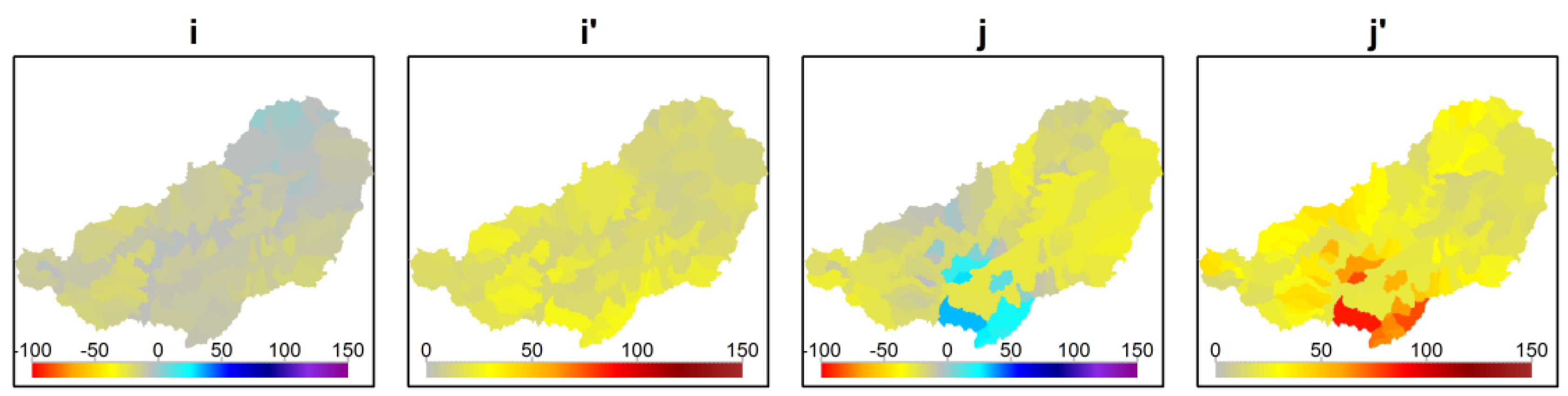
4.4. Spatial Assessment of Expected Changes


5. Conclusions
Acknowledgments
Author Contributions
Conflicts of Interest
References
- Poff, N.L.; Ward, J.V. Physical habitat template of lotic systems : Recovery in the context of historical pattern of spatiotemporal heterogeneity. Environ. Manag. 1990, 14, 629–645. [Google Scholar] [CrossRef]
- Contribution of Working Group I to the Fourth Assessment Report of the Intergovernmental Panel on Climate Change; Cambridge University Press: Cambridge, UK; New York, NY, USA, 2007.
- Climate Change and Water; Technical Paper of the Intergovernmental Panel on Climate Change (IPCC); IPCC Secretariat: Geneva, Switzerland, 2008; p. 202.
- Contribution of Working Group II to the Fourth Assessment Report of the Intergovernmental Panel on Climate Change; Cambridge University Press: Cambridge, UK, 2007; p. 976.
- Communication from the Commission to the European Parliament, the Council, the European Economic and Social Committee of the Region; European Union Strategy for Danube Region: Bruxsells, Belgium, 2010.
- Impacts of and Adaptation to Climate Change in the Danube-Carpathian Region. Overview Study Commissioned by the WWF Danube-Carpathian Programme; Department of Environmental Sciences and Policy, Central European University: Budapest, Hungary, 2008.
- Carpathian Integrated Assessment of Vulnerability to Climate Change and Ecosystem-Based Adaptation Measures (CARPIVIA) Projec Preliminary Assessment Vulnerability & Potential Adaptation Measures; Report Task 2; Dienst Landbouwkundig Onderzoek (DLO) Alterra: Wageningen, The Netherlands, 2011.
- Hamar, J.; Sarkany-Kiss, A. The Maros/Mureş River Valley. A Study of Geography, Hydrobiology and Ecology of the River and Its Environment; Tisza Klub for Environment and Nature: Szolnok, Hungary, 1995. [Google Scholar]
- Sandu, C.; Bloesch, J. The Mureş River ecosystem—Scientific background information as the basis for a catchment approach in the framework of IAD. In Proceedings of the 36th International Conference of IAD, Vienna, Austria, 4–8 September 2006.
- Rapid Environmental Assessment of the Tisza River Basin; United Nations Environment Programme (UNEP): Geneva, Switzerland, 2004.
- Nováky, B.; Bálint, G. Shifts and modification of the hydrological regime under climate change in Hungary. In Climate Change—Realities, Impacts Over Ice Cap, Sea Level and Risks; Singh, B.R., Ed.; InTech: Rjeka, Croatia, 2013. [Google Scholar]
- Bartholy, J.; Pongracz, R.; Miklos, E.; Kis, A. Simulated regional climate change in the Carpathian Basin using ENSEMBLES model simulations. In Proceedings of the 91st American Meteorological Society Annual Meeting, Seattle, WA, USA, 22–27 January 2011; p. 1117.
- Rakonczai, J. Effects and Consequences of Global Climate Change in the Carpathian Basin, Climate Change—Geophysical Foundations and Ecological Effects; Blanco, J., Ed.; InTech: Rijeka, Croatia, 2011. [Google Scholar]
- Danube River Basin—Climate Change Adaptation; Danube Study Report; Department of Geography, Ludwig-Maximilians-Universitaet: Munich, Germany, 2012.
- Sipos, G.; Blanka, V.; Mezősi, G.; Kiss, T.; Leeuwen, B.V. Effect of climate change on the hydrological character of River Maros, Hungary-Romania. J. Environ. Geogr. 2014, 7, 49–56. [Google Scholar] [CrossRef]
- United Nations Economic Commission for Europe UNECE Report No. 2: Mures/Maros: Identification and Review of Water Management Issues; Netherlands Institute for Inland Water Management and Waste Water Treatment: Lelystad, The Netherlands, 2002.
- Local Plan for Sustainable Development of Mures County; Romanian Government: Bucharest, Romania, 2005.
- Krysanova, V.; Müller-Wohlfeil, D.; Becker, A. Development and test of a spatially distributed hydrological/water quality model for mesoscale watersheds. Ecol. Model. 1998, 106, 261–289. [Google Scholar] [CrossRef]
- Van der Linden, P.; Mitchell, J. ENSEMBLES: Climate Change and Its Impacts: Summary of Research and Results from the ENSEMBLES Project; Met Office Hadley Centre: Exeter, UK, 2009. [Google Scholar]
- Richter, B.; Baumgartner, J.; Powell, J.; Braun, D. A method for assessing hydrologic alteration within ecosystems. Conserv. Biol. 1996, 10, 1163–1174. [Google Scholar] [CrossRef]
- Arnold, J.; Fohrer, N. SWAT2000: Current capabilities and research opportunities in applied watershed modelling. Hydrol. Process. 2005, 19, 563–572. [Google Scholar] [CrossRef]
- Krysanova, V.; Meiner, A.; Roosaare, J.; Vasilyev, A. Simulation modelling of the coastal waters pollution from agricultural watersched. Ecol. Model. 1989, 49, 7–29. [Google Scholar] [CrossRef]
- Krysanova, V.; Wechsung, F.; Arnold, J.; Ragavan, S.; Williams, J. SWIM—Soil and Water Integrated Model User Manual; PIK Report No. 69; PIK—Potsdam Institute for Climate Impact Research: Potsdam, Germany, 2000. [Google Scholar]
- Krysanova, V. Development of the ecohydrological model SWIM for regional impact studies and vulnerability assessment. Hydrol. Process. 2005, 19, 763–783. [Google Scholar] [CrossRef]
- Acreman, M.; Dunbar, M. Defining environmental river flow requirements—A review. Hydrol. Earth Syst. Sci. 2004, 8, 861–876. [Google Scholar] [CrossRef]
- Richter, B.; Mathews, R. Ecologically sustainable water management: managing river flows for ecological integrity. Ecol. Appl. 2003, 13, 206–224. [Google Scholar] [CrossRef]
- Gibson, C.; Meyer, J.; Poff, N. Flow regime alterations under changing climate in two river basins: Implications for freshwater ecosystems. River Res. Appl. 2005, 21, 849–864. [Google Scholar] [CrossRef]
- Richter, B.; Thomas, G. Restoring environmental flows by modifying dam operations. Ecol. Soc. 2007, 12, 1–26. [Google Scholar]
- SRTM 90m Digital Elevation Data. Available online: http://srtm.csi.cgiar.org/ (accessed on 31 March 2013).
- Corine Land Co ver 2000 Raster Data. Available online: http://www.eea.europa.eu/data-and-maps/data/corine-land-cover-2000-raster-2 (accessed on 31 March 2013).
- Weedon, G.; Gomes, S.; Viterbo, P.; Oestrle, H.; Adam, J.; Bellooin, N.; Boucher, O.; Best, M. The WATCH Forcing Data 1958–2001: A Meteorological Forcing Dataset for Land Surface and Hydrological Models; Technical Report No. 22; European Commission: Brussels, Belgium, 2010. [Google Scholar]
- Weedon, G.; Gomes, S.; Viterbo, P.; Shuttleworth, W.J.; Blyth, E.; Österle, H.; Adam, J.; Bellouin, N.; Boucher, O.; Best, M. Creation of the WATCH forcing data and its use to assess global and regional reference crop evaporation over land during the twentieth century. J. Hydrometeorol. 2011, 12, 823–848. [Google Scholar] [CrossRef]
- Nash, J.; Sutcliffe, J. River flow forecasting through conceptual models part I—A discussion of principles. J. Hydrol. 1970, 10, 282–290. [Google Scholar] [CrossRef]
- Krause, P.; Boyle, D.; Bäse, F. Comparison of different efficiency criteria for hydrological model assessment. Adv. Geosci. 2005, 150, 89–97. [Google Scholar] [CrossRef]
- Hesse, C.; Krysanova, V.; Päzolt, J.; Hattermann, F. Eco-Hydrological modelling in a highly regulated lowland catchment to find measures for improving water quality. Ecol. Modell. 2008, 218, 135–148. [Google Scholar] [CrossRef]
- Tebaldi, C.; Knutti, R. The use of the multi-model ensemble in probabilistic climate projections. Philos. Trans. R. Soc. 2007, 365, 2053–2075. [Google Scholar] [CrossRef] [PubMed]
- Weigel, A.P.; Knutti, R.; Liniger, M.A.; Appenzeller, C. Risks of model weighting in multimodel climate projections. J. Clim. 2010, 23, 4175–4191. [Google Scholar] [CrossRef]
- Hewitt, C.; Griggs, D. Ensembles-Based predictions of climate changes and their impacts. Eos Trans. Am. Geophys. Union 2004, 85, 566. [Google Scholar] [CrossRef]
- Moriasi, D.; Arnold, J.; van Liew, M.; Binger, R.; Harmel, R.; Veith, T. Model evaluation guidelines for systematic quantification of accuracy in watershed simulations. Trans. ASABE 2007, 50, 885–900. [Google Scholar] [CrossRef]
- Kendon, E.J.; Jones, R.G.; Kjellström, E.; Murphy, J.M. Using and designing GCM-RCM ensemble regional climate projections. J. Clim. 2010, 23, 6485–6503. [Google Scholar] [CrossRef]
- Hattermann, F.; Weiland, M.; Huang, S.; Krysanova, V.; Kundzewicz, Z. Model-Supported impact assessment for the water sector in Central Germany under climate change—A case study. Water Resour. Manag. 2011, 25, 3113–3134. [Google Scholar] [CrossRef]
- Lobanova, A.; Stagl, J.; Vetter, T.; Hattermann, F. Evaluation of flow alterations and sequential influence on the riverine ecosystem under climate change in the Mures River Basin, Romania. In Proceedings of the XXVI Conference of the Danubian Countries on Hydrological Forecasting and Hydrological Bases of Water Management, Deggendorf, Germany, 22–24 September 2014.
- Leipprand, A.; Kadner, S.; Dworak, T.; Hattermann, F.; Post, J.; Krysanova, V.; Benzie, M.; Berglund, M. Impacts of Climate Change on Water Resources—Adaptation Strategies for Europe; German Federal Environment Agency: Dessau-Roßlau, Germany, 2008. [Google Scholar]
© 2015 by the authors; licensee MDPI, Basel, Switzerland. This article is an open access article distributed under the terms and conditions of the Creative Commons Attribution license (http://creativecommons.org/licenses/by/4.0/).
Share and Cite
Lobanova, A.; Stagl, J.; Vetter, T.; Hattermann, F. Discharge Alterations of the Mures River, Romania under Ensembles of Future Climate Projections and Sequential Threats to Aquatic Ecosystem by the End of the Century. Water 2015, 7, 2753-2770. https://doi.org/10.3390/w7062753
Lobanova A, Stagl J, Vetter T, Hattermann F. Discharge Alterations of the Mures River, Romania under Ensembles of Future Climate Projections and Sequential Threats to Aquatic Ecosystem by the End of the Century. Water. 2015; 7(6):2753-2770. https://doi.org/10.3390/w7062753
Chicago/Turabian StyleLobanova, Anastasia, Judith Stagl, Tobias Vetter, and Fred Hattermann. 2015. "Discharge Alterations of the Mures River, Romania under Ensembles of Future Climate Projections and Sequential Threats to Aquatic Ecosystem by the End of the Century" Water 7, no. 6: 2753-2770. https://doi.org/10.3390/w7062753