
Application of a 3D Layer Integrated Numerical Model of Flow and Sediment Transport Processes to a Reservoir


Abstract
:1. Introduction
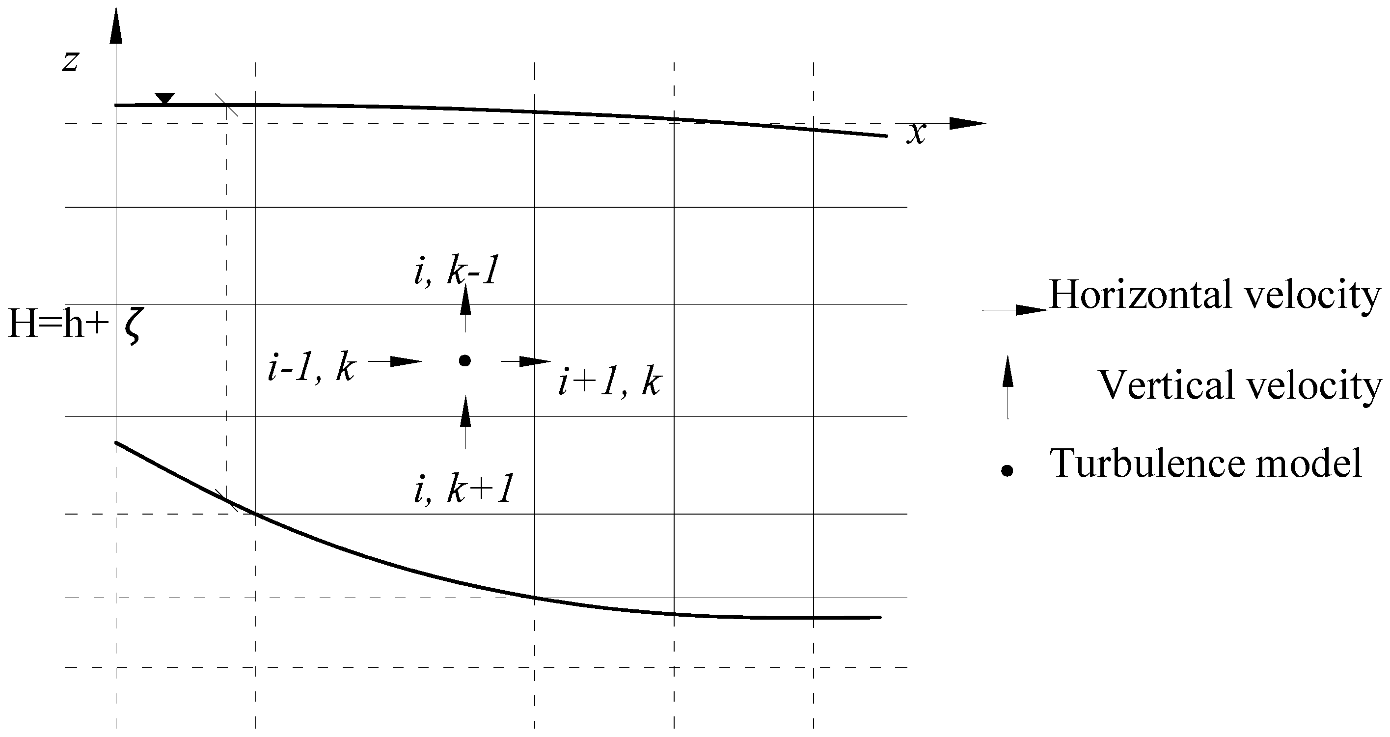
2. Governing Equations
2.1. Layer Integrated Hydrodynamic Model

2.2. Turbulence Model
2.3. Sediment Transport Model
3. Numerical Simulation
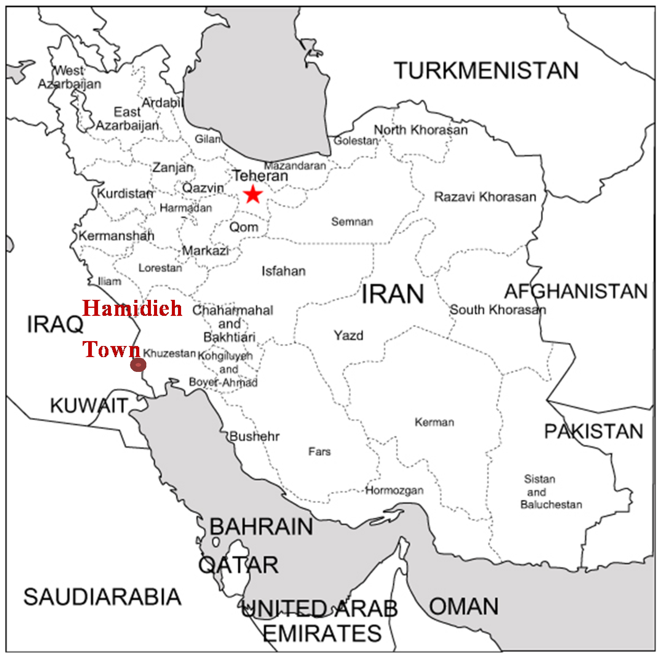
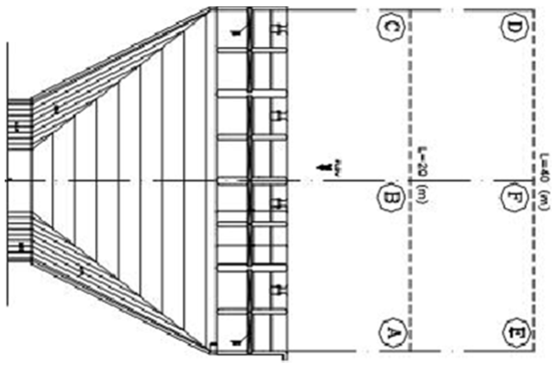
4. Model Application to Hamidieh Reservoir
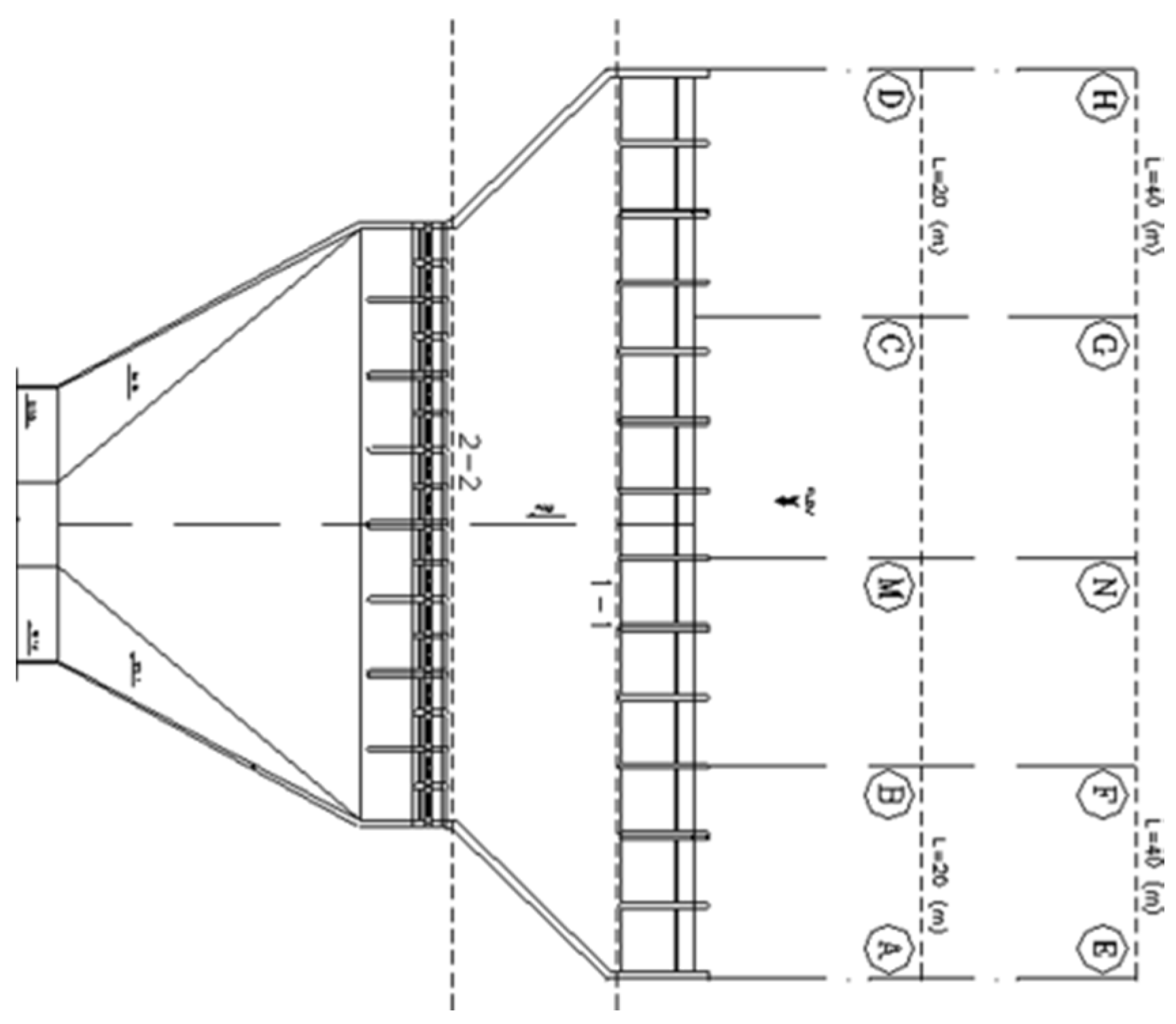
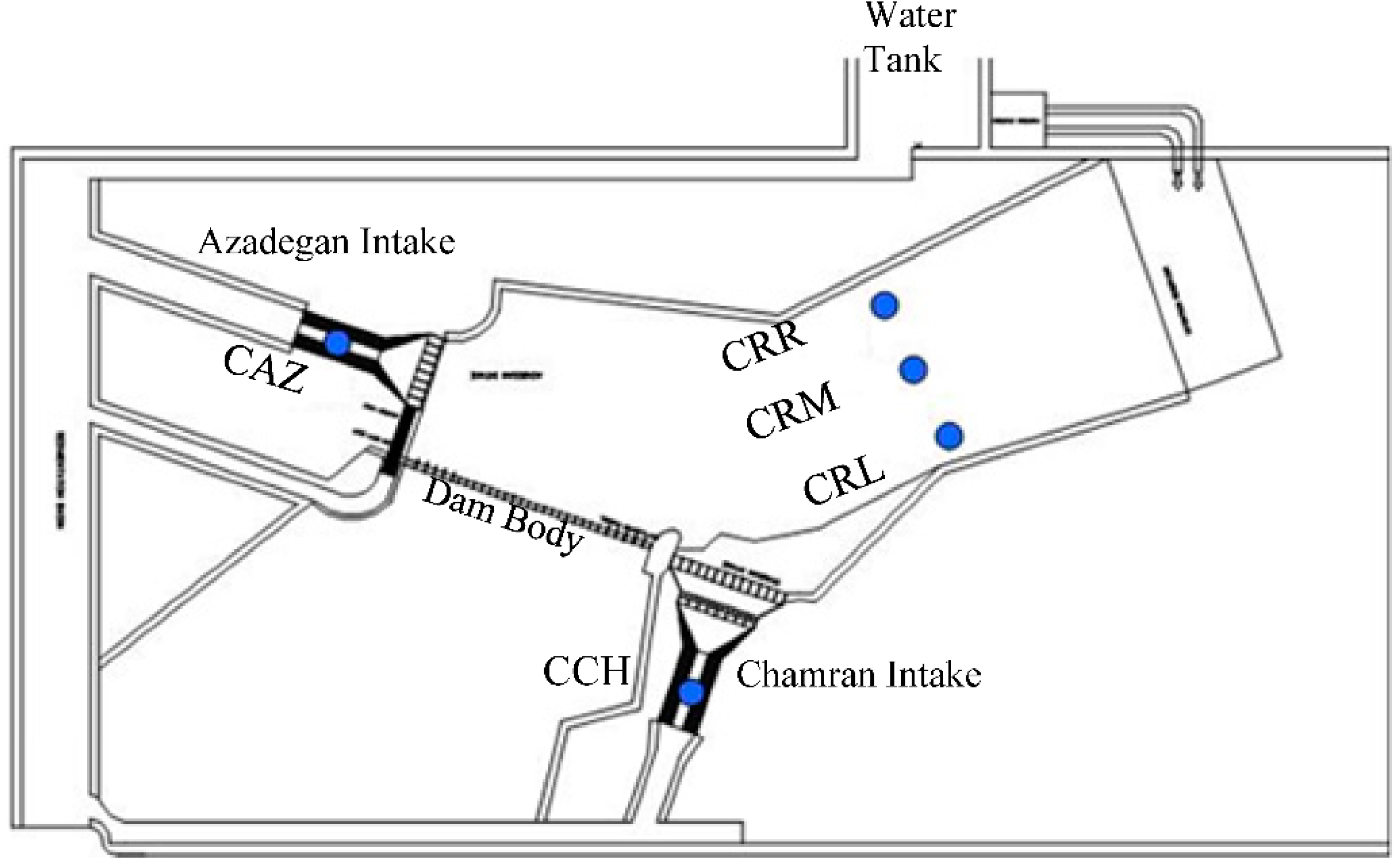
4.1. Project Background


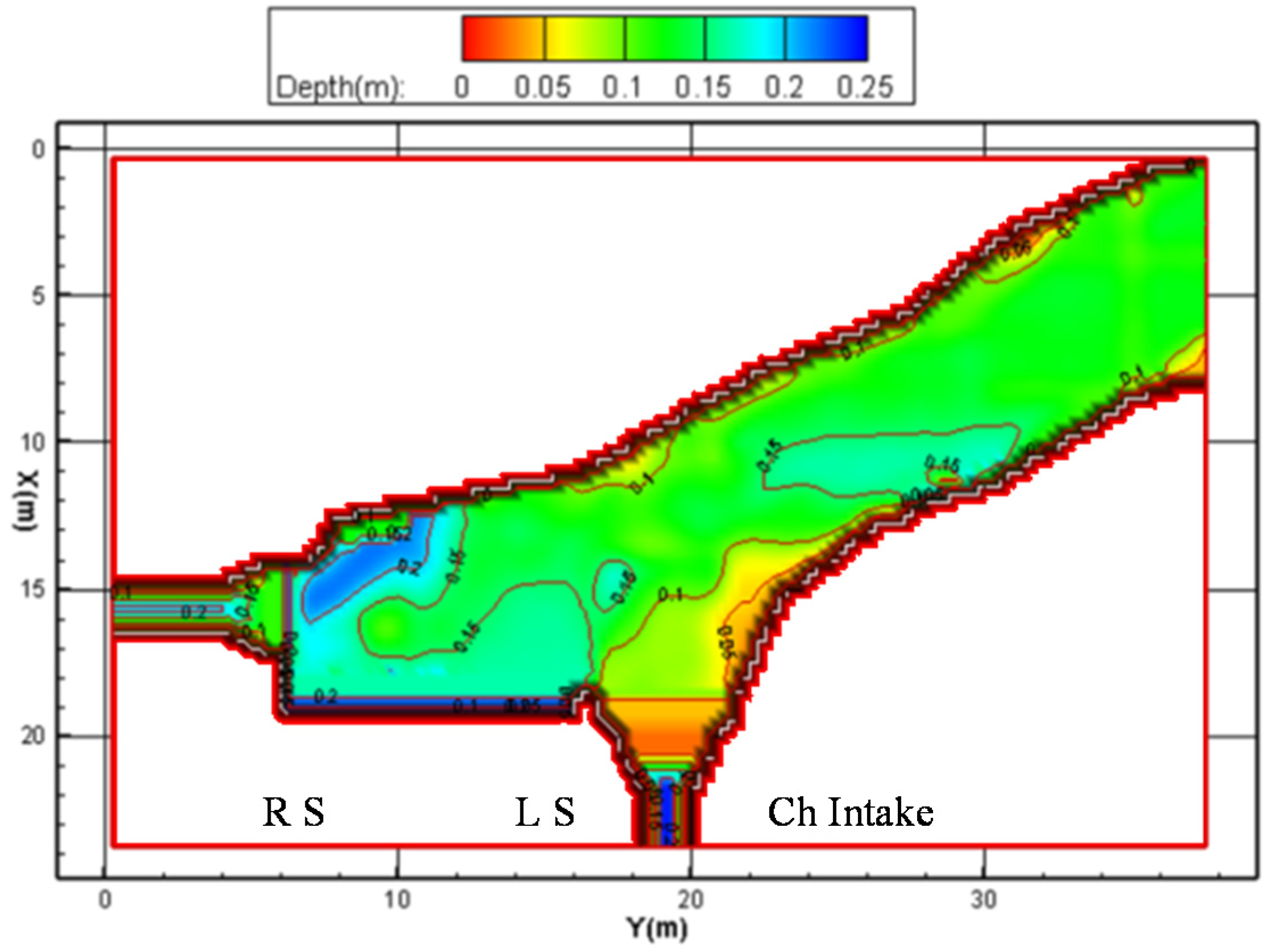
4.2. Numerical Model Simulation Details
4.2.1. Hydrodynamics


| Facility | Hydraulic Boundary Condition | Turbulence Boundary Condition | Operation |
|---|---|---|---|
| Reservoir | Discharge 82.2 L/s | Surface and Inlet | Water level (1.01 m) |
| Az Intake | Discharge 41.9 L/s | Outlet | – |
| Ch Intake | Water Level (1 m) | Outlet | – |
| LS | Closed | – | – |
| RS | Closed | – | – |


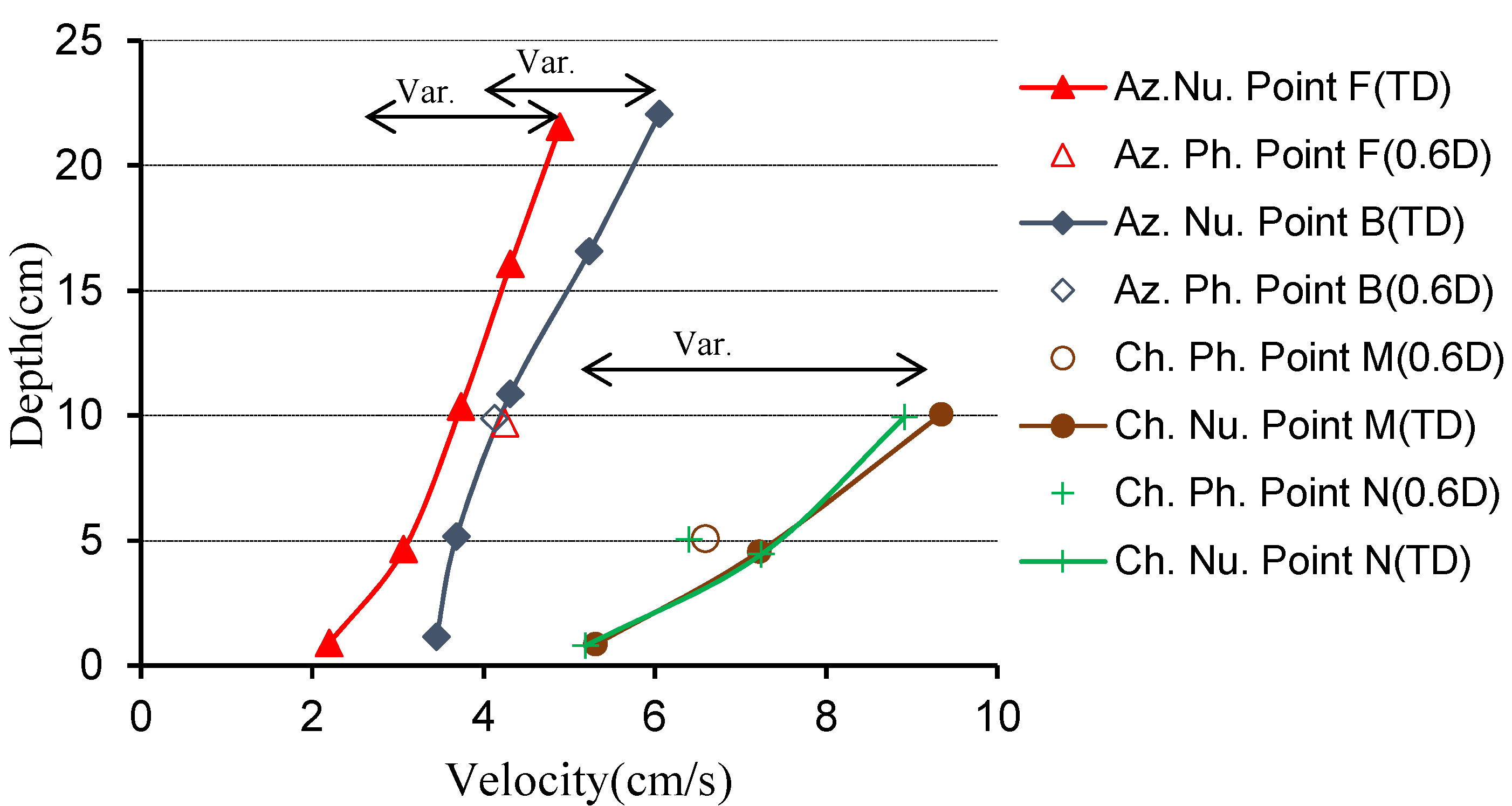
| Location | Points | Measured (cm/s) | Calculated (cm/s) |
|---|---|---|---|
| Chamran | A | 3.09 | 4.0 |
| B | 5.91 | 6.08 | |
| M | 6.59 | 7.21 | |
| C | 5.91 | 6.63 | |
| D | 3.10 | 3.89 | |
| E | 3.08 | 3.86 | |
| F | 5.27 | 5.94 | |
| N | 6.40 | 7.24 | |
| G | 5.18 | 6.53 | |
| H | 3.59 | 3.89 | |
| Azadegan | A | 3.97 | 4.70 |
| B | 4.13 | 4.31 | |
| C | 4.46 | 5.15 | |
| E | 3.18 | 3.54 | |
| F | 4.25 | 3.73 | |
| D | 3.18 | 3.59 |


| Scenario No. | Facility | Hydraulic Boundary Condition | Turbulence Boundary Condition | Operation |
|---|---|---|---|---|
| S2 | Reservoir | Discharge 92.2 L/s | Surface and Inlet | Water level (1.0225 m) |
| Az Intake | Discharge 41.9 L/s | Outlet | – | |
| Ch Intake | Water Level (1 m) | Outlet | – | |
| LS | Discharge 5.6 L/s | Outlet | – | |
| RS | Closed | – | – | |
| S3 | Reservoir | Discharge 135 L/s | Surface and Inlet | Water level (1.0225 m) |
| Az Intake | Discharge 41.9 L/s | Outlet | – | |
| Ch Intake | Water Level (1 m) | Outlet | – | |
| LS | Discharge 25.2 L/s | Outlet | – | |
| RS | Discharge 25.2 L/s | Outlet | v |
- -
- -
- -

4.2.2. Sediment Transport
- Low flow without sluice gates (S4).
- Low flow with one sluice gate (left-hand side) in operation (S5).
- High flow with sluice gates along both sides of the dam in operation (S6).

| Scenario No. | Facility | Operation | Boundary Condition | Concentration gr/L |
|---|---|---|---|---|
| S4 | Reservoir | Water level 1.0225 m | Discharge 87.2 L/s | 0.4724 |
| Az Intake | – | Discharge 41.9 L/s | – | |
| Ch Intake | – | Water level 1 m | – | |
| LS | – | – | – | |
| RS | – | – | – | |
| S5 | Reservoir | Water level 1.0225 m | Discharge 92.2 L/s | 0.6724 |
| Az Intake | – | Discharge 41.9 L/s | – | |
| Ch Intake | – | Water level 1 m | – | |
| LS | – | Discharge 5.6 L/s | – | |
| RS | – | – | – | |
| S6 | Reservoir | Water level 1.0225 m | Discharge 135 L/s | 1.3391 |
| Az Intake | – | Discharge 41.9 L/s | – | |
| Ch Intake | – | Water level 1 m | – | |
| LS | – | Discharge 25.2 L/s | – | |
| RS | – | Discharge 25.2 L/s | – |
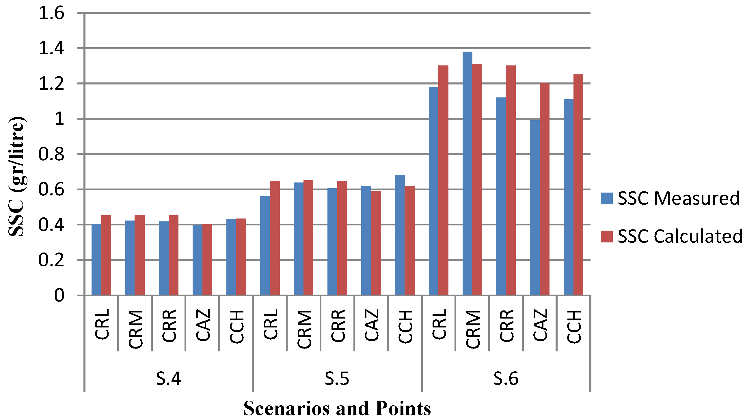
| Scenario No. | Points | SSC (Measured) gr/L | SSC (Calculated) gr/L | |Error| * % |
|---|---|---|---|---|
| S4 | CRL | 0.401 | 0.452 | 12.72 |
| CRM | 0.423 | 0.456 | 7.8 | |
| CRR | 0.417 | 0.452 | 8.39 | |
| CAZ | 0.396 | 0.401 | 1.26 | |
| CCH | 0.433 | 0.434 | 0.23 | |
| S5 | CRL | 0.563 | 0.645 | 14.56 |
| CRM | 0.638 | 0.651 | 2.04 | |
| CRR | 0.605 | 0.645 | 6.61 | |
| CAZ | 0.618 | 0.589 | 4.69 | |
| CCH | 0.681 | 0.619 | 9.10 | |
| S6 | CRL | 1.18 | 1.3 | 10.17 |
| CRM | 1.38 | 1.31 | 5.07 | |
| CRR | 1.12 | 1.3 | 16.07 | |
| CAZ | 0.99 | 1.20 | 21.21 | |
| CCH | 1.11 | 1.25 | 12.61 |
- -
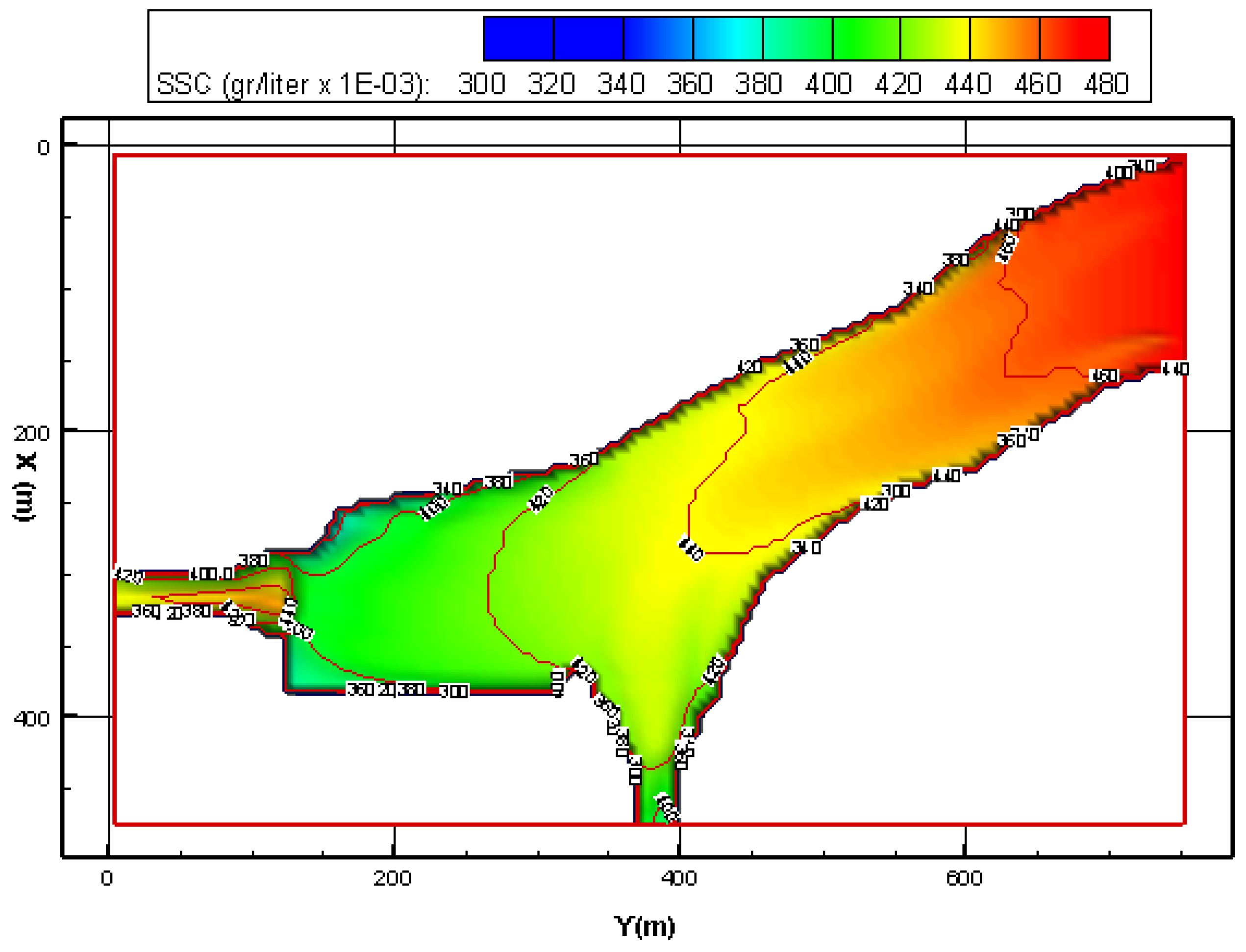
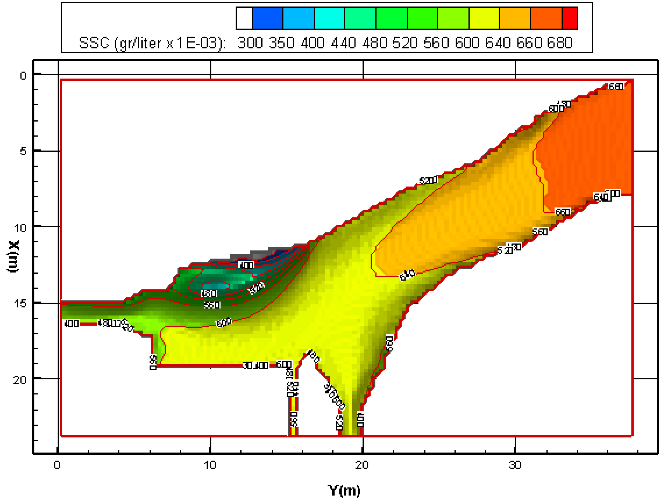
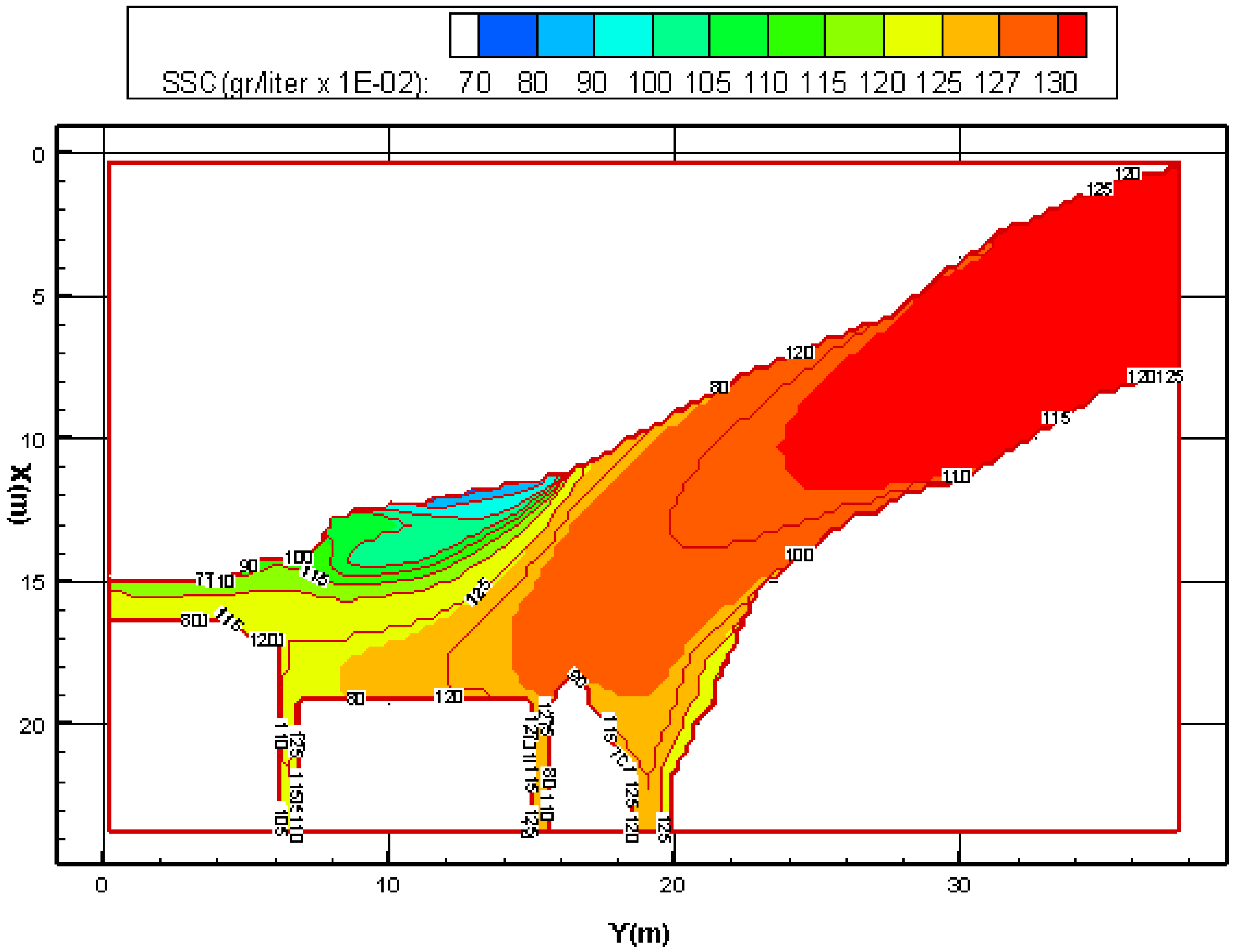
- The SSC in the Chamran intake is higher than that in the Azadegan intake (see CCH and CAZ in Table 5). This is due to the fact that the Chamran intake was located along the convex bank, where the flow velocity was greater than that at other locations across the cross-section.
- -
- The pattern of the suspended sediment movement in the reservoir shows that the sediment flux rate entering into the Chamran intake is not significantly affected by the intake gate and sluice gate operation schemes. This means that the sluice gates on the left-hand side do not have a considerable effect on reducing the SSCs passing through Chamran intake.
- -
- The problem of sediments entering the intakes (especially the Chamran intake) still exists. The performance of these hydraulic structures is only part of the reason for this problem. The dominant natural process of sediment transport (especially for the suspended load part) and the size of the sediment particles play an important role in connection with this problem. In mitigating against this problem, then, dredging and sediment control measures should be periodically undertaken at the upstream reach of the dam.


5. Conclusions
- The 3D layer integrated scheme used in the numerical model is capable of representing the governing three-dimensional hydrodynamic and solute transport processes with an encouraging level of accuracy for the cases considered. Due to the important role of the near-bed layer (with high sediment concentrations), the sediment transport processes obtained using the 3D layer integrated model is applicable for predicting the hydro-morphological processes in the natural environment. By using this method, the computational time has been reduced significantly.
- The computed SSC distributions predicted using the numerical model for Hamidieh Reservoir agreed well with the measurements taken from the physical model, with an average error of less than 8.3% (see Table 5). To acquire this level of accuracy, the hydrodynamic computational scheme and the selected turbulence model were found to be crucial. The results of this research showed that the selection of the k-ε turbulence model in reservoirs, where the Reynolds number is high, but without any significant local vortex near any hydraulic structures (such as gates), was the correct choice. An accurate estimation of the eddy viscosity had a direct impact on the calculated flow velocity distribution (both horizontally and vertically), and the mixing coefficient was found to be a key parameter in calculating the sediment transport fluxes.
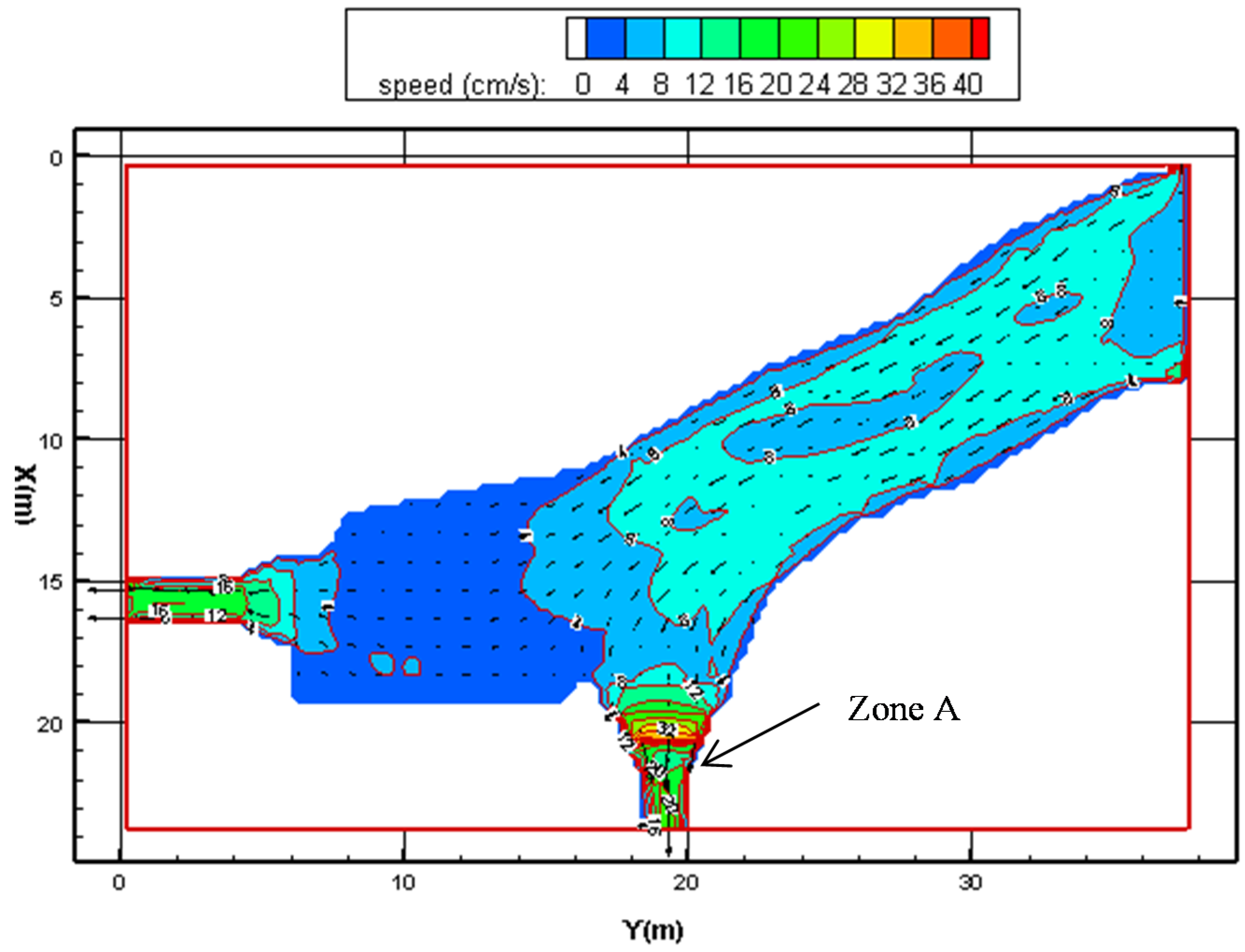
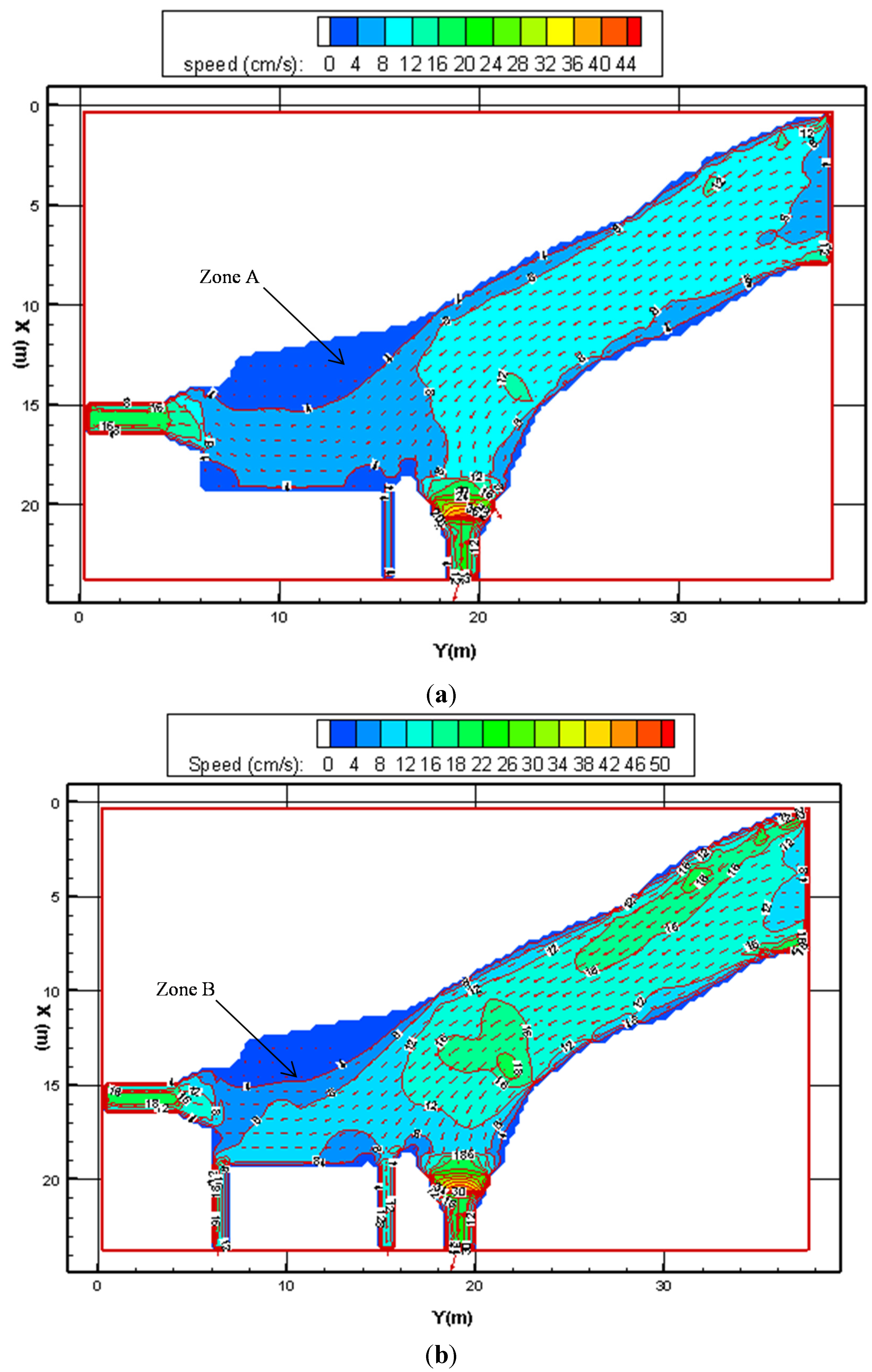
- The calibrated numerical model, set up for Hamidieh Reservoir, revealed many hydraulic aspects that were generally in good agreement with the physical model study results. Some of the important aspects are summarised below:
- -
- A non-uniform velocity distribution zone existed upstream of Chamran intake on the left-hand bank side. The flow velocity field near this intake showed more variations in comparison to the velocity distribution for Azadegan intake.
- -
- The recommended artificial dredging zone, located in front of the Azadegan intake, did not affect the hydraulic behaviour significantly.
- -
- The location of Chamran intake had a considerable impact on the SSCs moving through the intake.
- -
- The intake and sluice gate operation schemes had a relatively small impact on the suspended sediment fluxes entering Chamran intake.
- The results of this research have indicated that the calibrated numerical model could be used in the hydro-morphological design, operation and management of regulated reservoirs, particularly following the application of the model to the study reported herein. By using this approach, laboratory tests were reduced, and thus, time and budget considerations were optimized.
Acknowledgements
Author Contributions
Conflicts of Interest
References
- Galppatti, G.; Vreugdenhil, C.B. A depth-integrated model for suspended sediment transport. J. Hydraul. Eng. ASCE 1985, 127, 30–37. [Google Scholar] [CrossRef]
- Celic, I.; Rodi, W. Modelling suspended sediment transport in non-equilibrium situation. J. Hydraul. Eng. ASCE 1988, 114, 1157–1191. [Google Scholar] [CrossRef]
- O’Connor, B.A.; Nicholson, J. A three-dimensional model of suspended particulate sediment transport. Coast. Eng. 1988, 12, 157–174. [Google Scholar] [CrossRef]
- Lin, B.; Falconer, R.A. Three-dimensional layer integrated modelling of estuarine flows with flooding and drying. Estuar. Coast. Shelf Sci. 1997, 44, 737–751. [Google Scholar] [CrossRef]
- Van Rijn, L.C. Mathematical Modelling of Morphological Processes in the Case of Suspended Sediment Transport. Ph.D. Thesis, Delft Technical University, Delft, The Netherlands, June 1987. [Google Scholar]
- Van Rijn, L.C.; van Rossum, H.; Termes, P. Field verification of 2D and 3D suspended sediment models. J. Hydraul. Eng. ASCE 1990, 116, 1270–1278. [Google Scholar] [CrossRef]
- Olsen, N.R.B.; Skoglund, M. Three dimensional numerical modelling of water and sediment flow in a sand trap. J. Hydraul. Res. 1994, 32, 833–844. [Google Scholar] [CrossRef]
- Olsen, N.R.B. Three dimensional CFD modelling of free-forming meander channel. J. Hydraul. Eng. 2003, 129, 366–372. [Google Scholar] [CrossRef]
- Rüther, N.; Olsen, N.R.B. CFD modelling of alluvial channel instabilities. In Proceedings of The 3rd IAHR Symposium on River, Coastal and Estuarine Morphodynamics, IAHR, Barcelona, Spain, 1–5 September 2003.
- Rüther, N.; Olsen, N.R.B. Advances in 3D Modelling of Free forming Meander Formation from Initially Straight Alluvial Channels. In Proceeding of The 31st IAHR Congress, Seoul, Korea, 11–16 September 2005.
- Rüther, N.; Olsen, N.R.B. Three dimensional modeling of sediment transport in a narrow 90° channel bend. J. Hydraul. Eng. 2005, 131, 917–920. [Google Scholar] [CrossRef]
- Ruether, N.; Singh, J.M.; Olsen, N.R.B.; Atkinson, E. 3D computation of sediment transport at water intakes. Proc. Inst. Civ. Eng. Water Manage. 2005, 158, 1–8. [Google Scholar] [CrossRef]
- Khosronejad, A.; Rennie, C.D.; Salehi Neyshabouri, A.A. Three-dimensional numerical modeling of reservoir sediment release. J. Hydraul. Res. 2008, 46, 209–223. [Google Scholar] [CrossRef]
- Souza, L.B.S.; Schulz, H.E.; Villela, S.M.; Gulliver, J.S.; Souza, L.B.S. Experimental study and numerical simulation of sediment transport in a shallow reservoir. J. Appl. Fluid Mech. 2010, 3, 9–21. [Google Scholar]
- Hakimzadeh, H.; Falconer, R.A. Layer integrated modelling of three-dimensional recirculating flows in model tidal basins. J. Water Port Coastal Ocean Eng. 2007, 135, 324–333. [Google Scholar] [CrossRef]
- Lin, B.; Falconer, R.A. Three-dimensional layer integrated modelling of estuarine flows with flooding and drying. Estuar. Coast. Shelf Sci. 1997, 44, 737–751. [Google Scholar] [CrossRef]
- Nezu, I.; Nakagawa, A. Turbulence in Open Channel Flows; IAHR Monograph Series: Rotterdam, The Netherlands, 1993. [Google Scholar]
- Rodi, W. Large eddy simulation of river flows. In Proceedings of International Conference on Fluvial Hydraulics, IAHR, Braunscheweig, Germany, 8–10 September 2010.
- Fischer, H.B.; List, E.G.; Koh, R.C.Y.; Imberger, J.; Brooks, N.H. Mixing and Dispersion in Inland and Coastal Waters; Academic Press: Waltham, MA, USA, 1979. [Google Scholar]
- Hakimzadeh, H. Turbulence Modelling of Tidal Currents in Rectangular Harbors. Ph.D. Thesis, University of Bradford, Bradford, UK, July 1997. [Google Scholar]
- Krishnappan, B.G.; Lau, Y.L. Turbulence modelling of flood plain flows. J. Hydraul. Eng. 1986, 112, 251–266. [Google Scholar] [CrossRef]
- Van Rijn, L.C. Sediment transport, part I: Bed load transport. J. Hydraul. Eng. ASCE 1984, 110, 1431–1456. [Google Scholar] [CrossRef]
- Falconer, R.A.; George, G.D.; Hall, P. Three-dimensional numerical modelling of wind-driven circulation in a shallow homogeneous Lake. J. Hydrol. 1991, 124, 59–79. [Google Scholar] [CrossRef]
- Faghihirad, S.; Lin, B.; Falconer, R.A. 3D layer-integrated modelling of flow and sediment transport through a river regulated reservoir. In Proceedings of International Conference on Fluvial Hydraulics, IAHR, Braunscheweig, Germany, 8–10 September 2010; pp. 1573–1580.
- Faghihirad, S.; Lin, B.; Falconer, R.A. 3D layer-integrated modelling morphological changes in a river regulated reservoir. In Proceedings of the 7th IAHR Symposium on River, Coastal and Estuarine Morphodynamics (RCEM), Beijing, China, 6–8 September 2011.
© 2015 by the authors; licensee MDPI, Basel, Switzerland. This article is an open access article distributed under the terms and conditions of the Creative Commons Attribution license (http://creativecommons.org/licenses/by/4.0/).
Share and Cite
Faghihirad, S.; Lin, B.; Falconer, R.A. Application of a 3D Layer Integrated Numerical Model of Flow and Sediment Transport Processes to a Reservoir. Water 2015, 7, 5239-5257. https://doi.org/10.3390/w7105239
Faghihirad S, Lin B, Falconer RA. Application of a 3D Layer Integrated Numerical Model of Flow and Sediment Transport Processes to a Reservoir. Water. 2015; 7(10):5239-5257. https://doi.org/10.3390/w7105239
Chicago/Turabian StyleFaghihirad, Shervin, Binliang Lin, and Roger Alexander Falconer. 2015. "Application of a 3D Layer Integrated Numerical Model of Flow and Sediment Transport Processes to a Reservoir" Water 7, no. 10: 5239-5257. https://doi.org/10.3390/w7105239