Impacts of Climate Change on the Hydrological Regime of the Danube River and Its Tributaries Using an Ensemble of Climate Scenarios

Abstract

Information about the potential impacts of climate change on river runoff is needed to prepare efficient adaptation strategies. This study presents scenario projections for the future hydrological runoff regime in the Danube River Basin. The eco-hydrological watershed model Soil and Water Integrated Model (SWIM) was applied for the entire Danube River catchment, considering 1224 subbasins. After calibration and validation of the model, a set of high-resolution climate projections (bias-corrected and non-bias-corrected) served as meteorological drivers with which future daily river discharge under different climate warming scenario conditions was simulated. Despite existing uncertainties, robust trends could be identified. In the next 30 years, the seasonal stream-flow regime of the Danube and its tributaries is projected to change considerably. Our results show a general trend towards a decrease in summer runoff for the whole Danube basin and, additionally, in autumn runoff for the Middle and Lower Danube basin, aggravating the existing low flow periods. For the winter and early spring seasons, mainly January–March, an increase in river runoff is projected. Greater uncertainties show up in particular for winter runoff in the Dinaric Alps and the Lower Danube basin. The existing trends become very distinct until the end of the 21st century, especially for snow-influenced river regimes.

1. Introduction

River runoff is highly sensitive to climate, especially to changes in precipitation, snow regime and evapotranspiration [1,2]. Climate change will affect the hydrologic regime and river flow characteristics through changes in precipitation and evapotranspiration, as well as in the snow regime. [1].

The future development of the river runoff conditions, as a consequence of climate change, is of great interest for stakeholders and decision makers in the riparian states. Information about potential impacts is needed for consolidated impact assessments and for long-term planning and adaptation (i.e., National Communications of the United Nations Framework Convention on Climate Change). In Europe, discussions arose around how changes in water resources and river runoff can be considered in river basin management plans, as they are required by the European Water Framework Direction (WFD) [3].

The Danube River Basin is home to more than 80 million people and comprises a catchment area of 817,000 km² [4]. The river plays an important economic role in transportation, hydropower generation and water supply and bears unique ecological and cultural values. Being the second largest river in Europe, it comprises parts of 19 countries, which have to cooperate, according the WFD, in river basin management planning [5]. From a climatic point of view, the region embraces alpine and continental climates with a close connection to the Mediterranean region. The alpine and Mediterranean regions are seen as primary global hot spots of climate change in terms of amplified projected change [6].

However, regional climate models (RCMs) normally do not consider the entire hydrological cycle and are generally not able to reproduce observed long-term seasonal river runoff in a satisfactory way [7]. Hence, information from climate models cannot be used for hydrological impact assessment directly. The state-of-the-art approach to assessing potential climate change impacts on hydrology is through the use of hydrological models under climate scenario conditions derived from various combinations of climate models and scenarios in order to quantify the range of possible impacts [1,8,9]. The inter-model spread of the simulated outcomes is the first measure of model uncertainty [10]. Additionally, multi-model ensembles have the advantage of being able to sample structural uncertainties, although the models are not completely independent, as they share common components [11]. Subsequently, the range of different model projections is not necessarily bound in the range of uncertainty in the prediction [11].

In the literature, there are some climate impact studies in the Danube basin focusing on water resources at a regional level. In the Upper Danube region, climate change impacts have been investigated in major research programs (KLIWAS, AdaptAlp, ECCONET, GLOWA-Danube). Several studies using this approach have been conducted focusing on the Upper Danube catchment [12,13,14].

However, in many regions of the Danube catchment, very few impact studies using future scenario projections in combination with a hydrological model are available, and the existing ones mostly focus on small regions and do not use a range of climate scenarios [15]. In particular, little is known about climate change impacts on the river runoff and water resources of the Lower basin and some important tributaries, like the Sava and Velika Morava [15]. No impact study currently exists that investigates potential seasonal changes in the hydrological regime of the whole Danube River Basin consistently at a regional resolution using a uniform modeling approach.

The objective of this study is to gain robust scenario information about future river flow characteristics in the Danube catchment. Performing the first hydrological climate impact assessment for the whole Danube River catchment using a regional eco-hydrological model, this paper aims to:

(1)

Identify climate change impacts on runoff seasonality in the Danube catchment that are projected robustly among the different climate scenarios;

(2)

Provide hydrological scenario information for regions where only little information about possible climate change impacts on river runoff is available so far;

(3)

Apply a broad variety of climate scenarios to exhibit the climate model uncertainty.

To achieve these objectives, we set up a regional hydrological model for the entire Danube catchment. After calibration and validation of the model, a variety of climate scenarios was used as drivers to evaluate climate-driven changes in the seasonal river runoff dynamics for the near (2031–2060) and far future (2070–2100). The selected climate scenarios include fourteen climate models (non-bias corrected) within the SRES A1B scenario, as well as five global climate models (bias-corrected) within three different representative concentration pathways (RCP2.6, RCP6.0 and RCP8.5) (see Section 3.1).

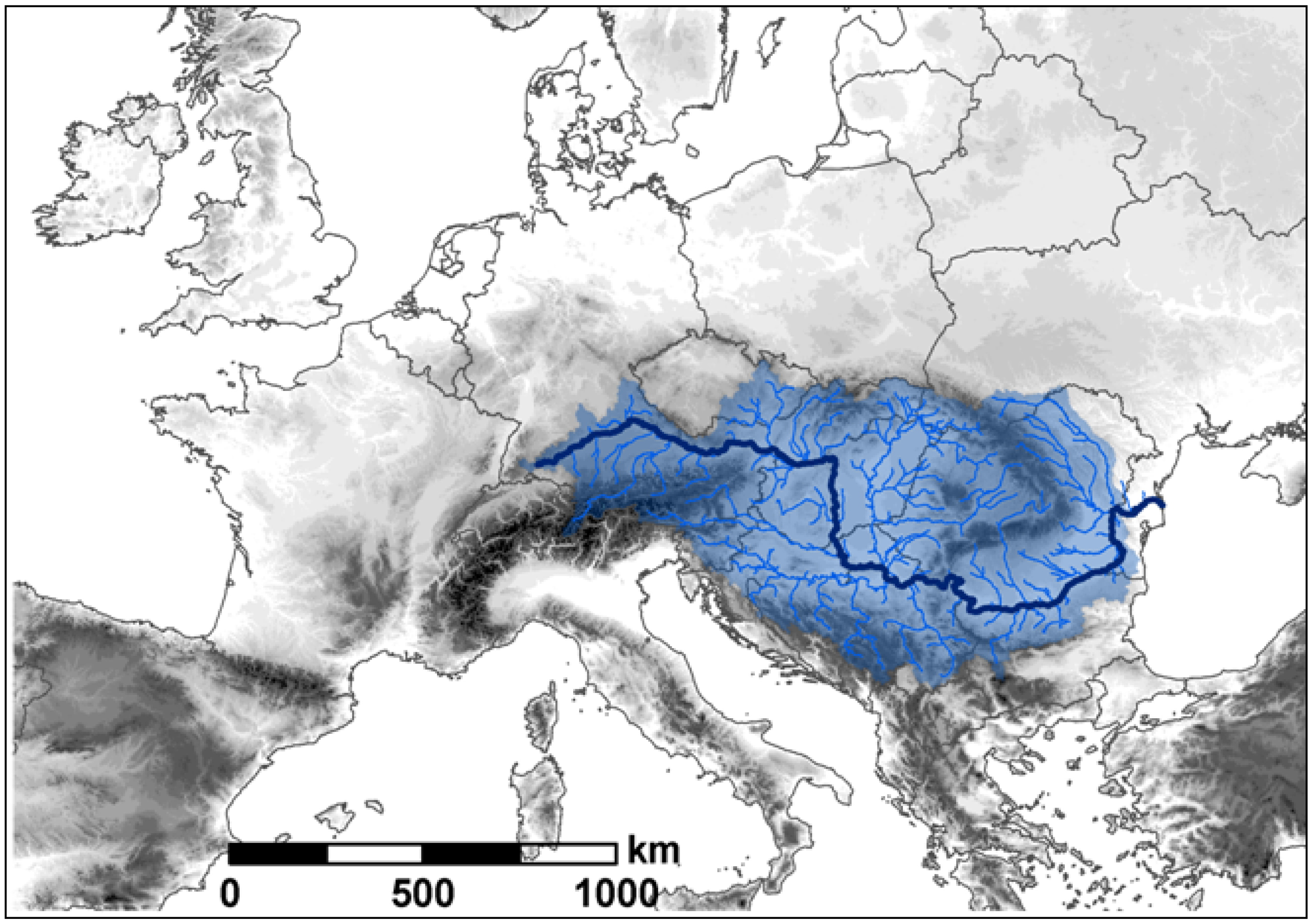
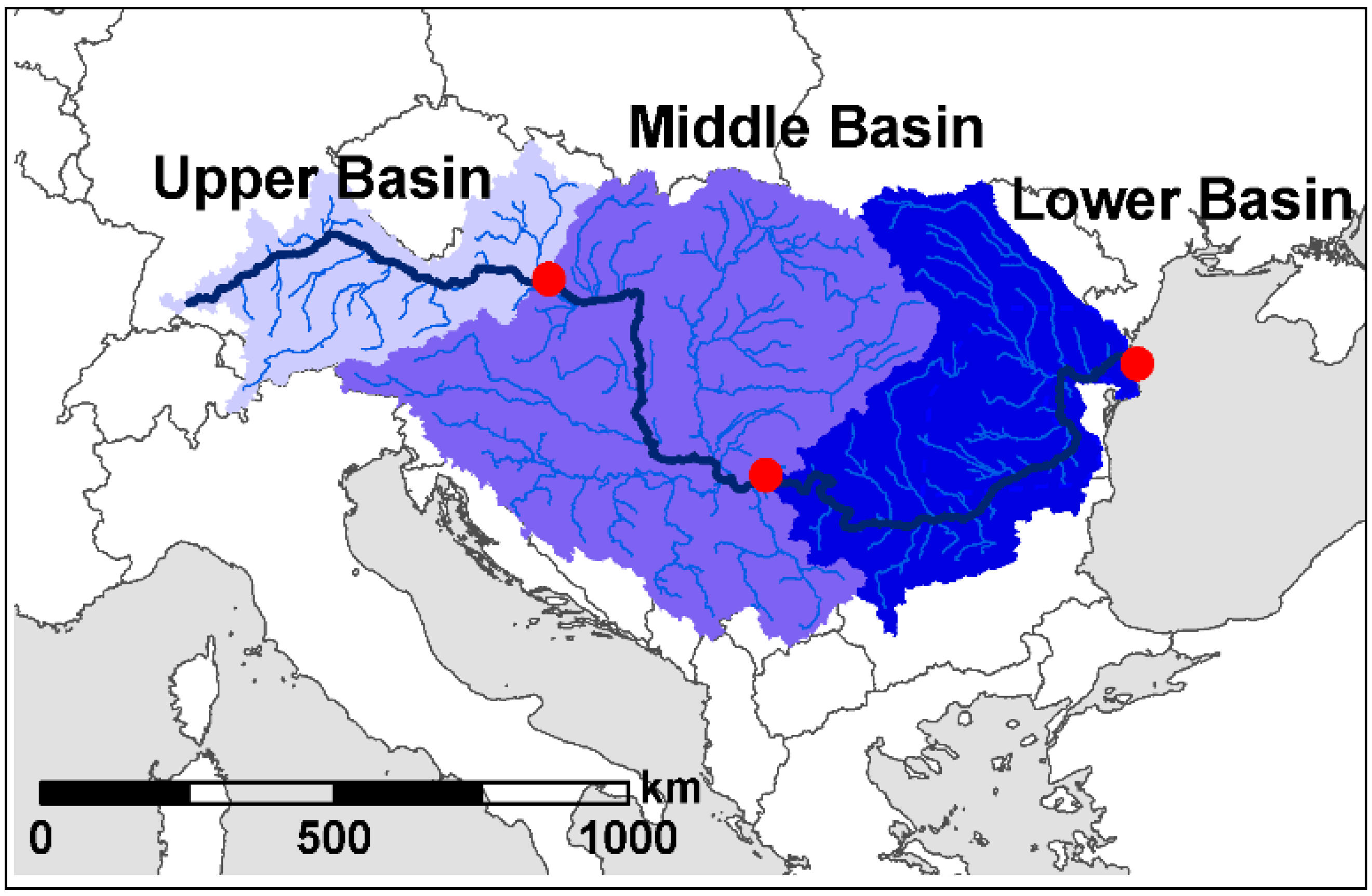
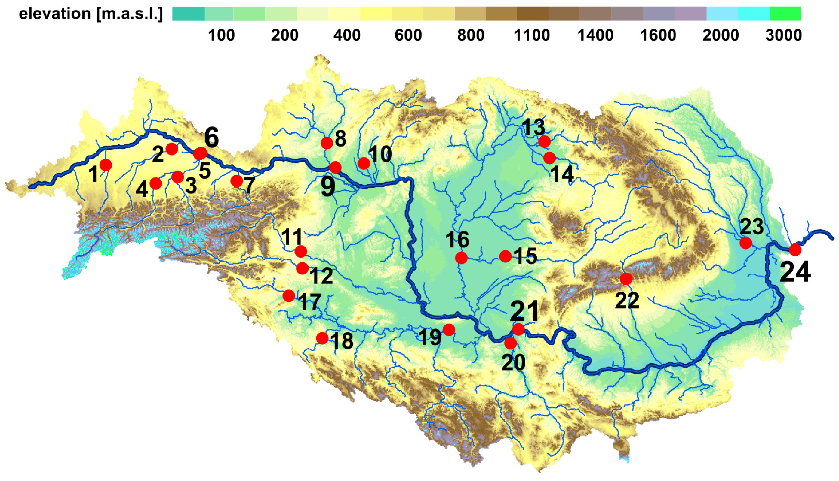
2. Study Area: The Danube River Catchment

The Danube is the second largest river in Europe, with a total length of 2826 km and a basin area of ~801,000 km² (see Figure 1). With 11 major tributaries, the Danube basin comprises parts of 19 countries (Germany, Austria, Switzerland, Italy, Slovenia, Slovakia, Hungary, Romania, Croatia, Serbia, Montenegro, Bulgaria, Moldova, Poland, Czech Republic, Bosnia-Herzegovina, Albania, FYR of Macedonia) and is hence the most international river basin in the world [4]. The Danube basin includes glacier-covered mountains in the Alps, the mid-mountains mostly covered with dense forests, karst regions with little vegetation, uplands, lowlands and wide plains [16]. The Danube River has its source at the confluence of the Breg and Brigach Rivers near Donaueschingen in the Black Forest (Germany) and flows from East to West into the Black Sea within a wide delta shared by Romania and Ukraine. Along the way, the slope decreases from 0.4% in the Alps to 0.004% right before the delta. [4]. Elevation ranges from 4052 m asl (Piz Bernina, Switzerland) to 0 m asl, with an average altitude of 458 m. The Alps in the west, the Dinaric-Balkan mountain chains in the south and the Carpathian Mountains receive the highest annual precipitation (1000–2000 mm); the Vienna basin, the Pannonian basin, the Romanian and Prut low plains, as well as the Danube delta receive rather low precipitation (<600 mm), in contrast [17].

In the Danube basin, the three major subsections of the Upper, Middle and Lower basin are distinguished (Figure 2). The Upper Danube basin goes from the source until the confluence with the Morava River near Bratislava (the so-called “Porta Hungarica”). It is characterized by an Atlantic climate with high precipitation. The major southern tributaries drain the alpine subbasins (Iller, Lech, Isar, Inn, Salzach, Traun and Enns) and the Morava River from the north [4]. The major tributary in the Upper Danube basin is the Inn River (mean annual discharge (MQ) at Passau-Ingling ~735 m³/s), which more than doubles the flow of the Danube at Passau [16]. Glacier cover in the Danube catchment is very limited and concentrated to the alpine Inn River catchment, where 1.41% of the area is glacier covered [18]. The annual contribution of glacier melt to the runoff at Passau after the confluence with the Inn River is 2% (1991–2000) [19].

Figure 1. Study area: the Danube River catchment in Europe.

Figure 1. Study area: the Danube River catchment in Europe.

Figure 2. The Danube River catchment divided into the Upper Danube basin (until the Bratislava station), the Middle Danube basin (until the Bazias station) and the Lower Danube basin (until the Ceatal Izmail station).

Figure 2. The Danube River catchment divided into the Upper Danube basin (until the Bratislava station), the Middle Danube basin (until the Bazias station) and the Lower Danube basin (until the Ceatal Izmail station).

The Middle Danube basin extends from Bratislava until the Iron Gates at the boundary between Serbia and Romania. After Bratislava, the slope of the Danube River decreases substantially at the Pannonian plain. The major tributaries in the north are the Váh and Hron Rivers (Slovakia) and the Tisza River coming from the Carpathian Mountains. From the south, there are the Leitha, Raab, Drava, Sava and Velika Morava. The climate is continentally influenced, with dry and cold winters and low precipitation. The Mediterranean climate influences parts of the Sava and Drava Rivers [4]. The Sava River (MQ at Sremska Mitrovica ~1570 m³/s), as the largest tributary of the Danube, contributes ~25% to the total runoff of the Danube, while the Tisza River (MQ at Szeged ~840 m³/s), the largest subbasin (138,408 km²) of the Danube by area (~12%), contributes only 12% to the runoff [16].

The Lower Danube basin drains the Romania-Bulgarian Lowlands via the Danube delta to the Black Sea. After passing the Carpathians, the Danube forms a lowland river system with formally wide floodplains [4]. The major tributaries, the source of which is in the Carpathian Mountains, are the Olt (MQ at Stoenesti 172 m³/s), Siret (MQ at Lungoci 210 m³/s) and Prut (MQ at Cernovci 67 m³/s) [16]. In the Lower basin, only ~1000 m³/s is added to the Danube River runoff (MQ). The mean annual runoff at the entrance to the Danube delta (at Ceatal Izmail station) adds up to ~6480 m³/s.

The largest dams in the Danube are Iron Gate Dams I and II constructed in 1972 and 1984, respectively, with a volume of 2.1 km³. Compared to the mean annual inflow to the reservoir at Bazias (~5460 m³/s), the degree of regulation (storage capacity/mean annual inflow) by this dam is less than 2% per year. Zaharia [20] found minor monthly deviations between the natural and regulated regimes at the Iron Gate dams, with a slight increase in discharges during low water periods (December–February and September/October) of +2% and a minimal decrease (of −1%) when the waters are high (May–August and November). Hence, despite the large storage volume, the Iron Gate dams are not significantly influencing the runoff regime on a monthly basis at the multiannual scale.

When analyzing changes in the historic runoff of the Danube at Ceatal Izmail (at the entrance to the Danube delta) since the 1930s, the present-day spring floods tend to come earlier and more distinctly, the summer runoff is reduced and the low flows in autumn are less distinct compared to those of the early 20th century (Figure 3). These historic shifts in seasonal discharge can be attributed to historic climate warming, water management activities, as well as land use change.

Figure 3. Historic changes in the long-term seasonal runoff of the Danube River at the entrance to the Danube delta (Ceatal Izmail station).

Figure 3. Historic changes in the long-term seasonal runoff of the Danube River at the entrance to the Danube delta (Ceatal Izmail station).

3. Methodology and Data

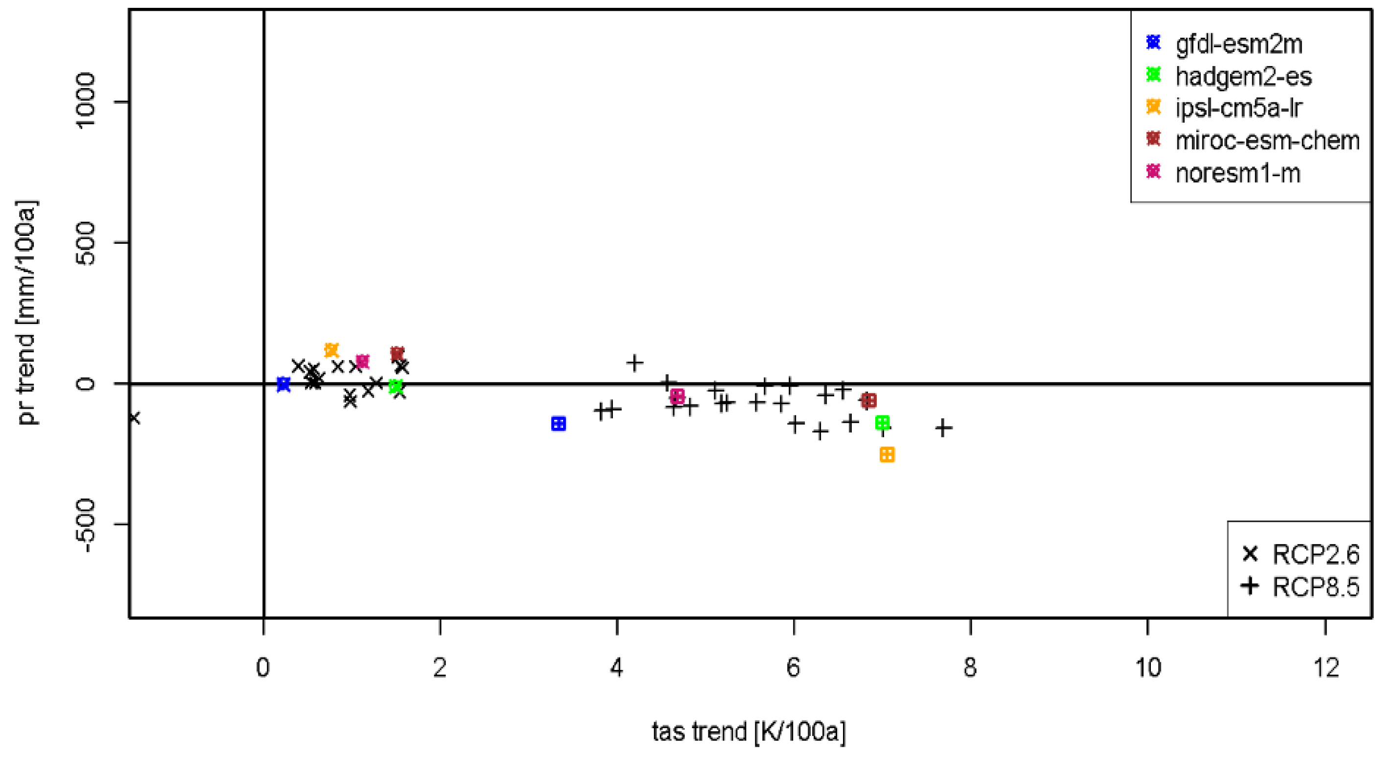
3.1. Climate Change Projections

3.1.1. ENSEMBLES Climate Models

As climate input data, we used high-resolution climate model simulations performed by several state-of-the-art global climate models (GCMs) and regional climate models (RCMs). Fourteen GCM/RCM combinations from the EU-FP6 ENSEMBLES project [21] were selected [22], all for the SRES A1B emission scenario with a resolution of ~25 km. The ENSEMBLES data under A1B SRES refer to a global warming level compared to that preindustrially (1850–1900) of approximately +3 °C until 2071–2100 and of +2 °C until 2031–2060.

The multi-model dataset consists of four GCMs (HadCM3, ECHAM5, Arpege and BCM), including three different realizations of HadCM3 and eight regional models (RCA3 (C4I), HIRHAM5, CLM3.21, HadRM3 (three realizations: Q0, Q3, Q16), REGCM3, RACHMO2, M-REMO and RCA3 (SMHI)). The climate scenario data come with all of the required parameters for hydrological analysis and are available from 1961–2100. For the HadCM3 GCM and the HadRM3 RCM, three realizations were included for “normal” climate sensitivity (Q0), “low” climate sensitivity (Q3) and “high” climate sensitivity (Q16) to the external greenhouse gas concentration forcing. In the climate simulations of the Met Office Hadley Center’s models, each year has 360 days with a standardized length of 30 days per month. To make them comparable to the other climate model data, the data are adjusted to 365 days in the calculations of the yearly and monthly (mean) values.

Jacob et al. [23] showed that the main systematic biases of the ENSEMBLES climate models vary across different models, seasons and regions. The comparison of the regional climate models for the interannual performance revealed distinct biases for temperature and precipitation (see Figure 4) for the historic conditions (WATCH data [24]). For temperature, the course of seasonality is represented adequately in all climate simulations with the right timing, but precipitation often shows a shift of one or two months. These biases in the meteorological driving data of the hydrological model are partly sustained in the runoff simulations, as shown here for the reference period (Figure 5).

The question of whether or not to apply a bias correction to overcome these biases in the climate models is widely discussed in the scientific community [25,26,27]. Bias correction is mostly limited to temperature and precipitation and leads (by definition) to a better agreement with the historical observations. This is in particular relevant for non-linear hydrological processes, like snow-water equivalent [28]. On the other hand, bias correction methods affect the advantages of dynamic climate models, like the tempo-spatial coherence of the climate variables (covariance structure) and the compliance of physical conservation principles [27,28]. Additionally, bias corrections are based on the assumption that statistical errors remain stationary in the future, but the bias will not necessarily stay the same in the next decades [25,26,27,28,29]. Hence, it is not certain if a bias correction leads to more realistic results in hydrological impact studies [30]. Muerth et al. [26] showed that bias- and non-bias-corrected climate model data lead to similar results in the climate change signal of runoff simulations for most indicators, except the timing of the spring flood peak.

Figure 4. Comparison for the years 1971–2000 of ENSEMBLES [21] regional climate model (RCM) data with historic observations (WATCH data [24]) for the Upper, Middle and Lower Danube basin. The thick black line shows the historic seasonality. The attribution of the different colors to the climate models is shown in Figure B1 (Appendix B).

Figure 4. Comparison for the years 1971–2000 of ENSEMBLES [21] regional climate model (RCM) data with historic observations (WATCH data [24]) for the Upper, Middle and Lower Danube basin. The thick black line shows the historic seasonality. The attribution of the different colors to the climate models is shown in Figure B1 (Appendix B).

Figure 5. Comparison for the years 1971–2000 of simulated river discharge with ENSEMBLES [21] RCM data with historic observations for the Danube station Bratislava (Upper Danube basin) and the Danube station Ceatal Izmail at the Danube Delta. The thick black line shows the measured discharge.

Figure 5. Comparison for the years 1971–2000 of simulated river discharge with ENSEMBLES [21] RCM data with historic observations for the Danube station Bratislava (Upper Danube basin) and the Danube station Ceatal Izmail at the Danube Delta. The thick black line shows the measured discharge.

We evaluated the non-bias-corrected RCM data from the ENSEMBLES project using a change signal approach. The climate change signal in the data is analyzed in the sense of the changes of each respective GCM/RCM run for a future scenario period compared to its simulations at the reference period (1971–2000). In this study, all climate models are considered equally. There is no established way to determine which climate model presents the most probable representation of the future [31]. Simulating the past and present correctly does not guarantee that the models will be correct in the future, as they could be “right for the wrong reasons” [7,32].

3.1.2. ISI-MIP Climate Models

To analyze the climate trends, we additionally used data provided by the Inter-Sectoral Impact Model Intercomparison Project (ISI-MIP [33]). The ISI-MIP project was designed to synthesize impact projections in the agriculture, water, biome, health and infrastructure sectors at different levels of global warming. Bias-corrected climate data are provided as input for the impact simulations from five GCMs of the “Coupled Model Intercomparison Project Phase 5” (CMIP5 ESMs): HadGEM2-ES, IPSL-CM5A-LR, MIROC-ESM-CHEM, GFDL-ESM2M and NorESM1-M [34]. The available global climate model outputs have been bi-linearly interpolated in space to a 0.5° × 0.5° grid and are available for the time period 1950–2099 [34]. The five Earth System models have been bias-corrected with a trend-preserving approach against the reanalysis WATCH dataset [24,34]. The WATCH dataset is therefore most suitable for the calibration of the hydrological model. Three “representative concentration pathways” (RCP) per GCM have been selected: RCP8.5, RCP6 and RCP2.6. The ISI-MIP scenarios refer to a global warming level compared to that preindustrially (1850–1900) until the end of the century (2071–2100) of approximately +2 °C (RCP2.6), +3 °C (RCP6.0) and +4 °C (RCP8.5). For the scenario period 2031–2060, the ISI-MIP scenarios correspond to a global warming level compared to that preindustrially of approximately +1.5 °C (RCP 2.6), +2.0 °C (RCP6.0) and +2.5 °C (RCP8.5).

Figure 6 shows the trends in precipitation and temperature until the end of the century of the ISI-MIP scenario runs in comparison to the outcome of a larger set of GCM runs used in the latest report of the IPCC Fifth Assessment Report. The five ISI-MIP model runs adequately cover the range of total GCM variation.

3.2. Eco-Hydrological Model SWIM

To study the potential effects of climate change on the hydrological conditions in the Danube basin, the eco-hydrological model SWIM (Soil and Water Integrated Model) has been chosen. SWIM is a process-based, semi-distributed watershed model [35] and integrates various coupled sub-modules for hydrology, plant growth, nutrient dynamics (nitrogen and phosphorus) and erosion using meteorological, topographical, land use, soil, vegetation and agricultural management input data as forcing datasets. The model operates on a daily time step and has proven to be suitable for the analysis of climate change and land use change impacts on hydrology [35], as well as for model-supported river basin management [36].

Figure 6. Trends in precipitation and temperature for the Danube region as simulated by 23 GCMs until the end of this century. The x-axis shows the global warming trend of a respective GCM simulation until the end of the 21st century compared to that preindustrially (1850–1900) in Kelvin/100 years. The y-axis shows the corresponding precipitation trend. In color: the five selected Inter-Sectoral Impact Model Intercomparison Project (ISI-MIP) [33] scenario runs for representative concentration pathways RCP2.6 and RCP8.5.

Figure 6. Trends in precipitation and temperature for the Danube region as simulated by 23 GCMs until the end of this century. The x-axis shows the global warming trend of a respective GCM simulation until the end of the 21st century compared to that preindustrially (1850–1900) in Kelvin/100 years. The y-axis shows the corresponding precipitation trend. In color: the five selected Inter-Sectoral Impact Model Intercomparison Project (ISI-MIP) [33] scenario runs for representative concentration pathways RCP2.6 and RCP8.5.

The SWIM model comprises a three-level disaggregation scheme from the watershed to subbasins and hydrotopes (hydrological response units). Each so-called hydrotope is considered spatially homogeneous in its parameter values for land use type, soil type, elevation and subbasin area. Hence, they are assumed to respond hydrologically in a uniform way. The hydrological module is based on the water balance equation, including precipitation, evaporation, transpiration, percolation, surface and subsurface runoff. Four subsystems are implemented in SWIM’s hydrological module: ground surface, root zone (soil profile) and shallow and deep groundwater reservoirs. The vegetation module is based on a simplified EPIC (Erosion Productivity Impact Calculator) approach [37] for natural vegetation and crop types. During the simulation, water flows are calculated on the hydrotope level. These are added up for each subbasin, and the lateral flows of water, sediments and nutrients are then routed following the river network based on the Muskingum routing procedure, taking transmission losses into account. SWIM includes an enhanced snow module for snow accumulation and snow melt processes, including a finer spatial resolution within the subbasin [38]. The glacier module [38] is based on the degree-day method, which is seen to be sufficient for studies on catchment scale [39].

3.2.1. Input Data for Hydrological Modelling

As input for the eco-hydrological model, digital elevation, land use and soil data are required, as climate forcing data, daily precipitation, temperature, solar radiation and relative humidity need to be provided on a daily basis. All spatial raster data were adjusted to a grid resolution of 440 × 440 m.

The digital elevation model (DEM) used here was provided by the Shuttle Radar Topographical Mission [40]. It is provided as 15 s × 15 s mosaic sets.

Land use data were reclassified from the CORINE 2000 classification [41] with a resolution of 100 × 100 m. The CORINE 2000 is based on LANDSAT 7 ETM satellite images (years 1999–2002). For the hydrological model, the CORINE 2000 types are translated to 15 land use categories (water, settlement, industry, road, bare soil, cropland, meadow, pasture, set-aside, evergreen forest, deciduous forest, mixed forest, wetland, heather and glaciers).

The soil parameters are based on the Harmonized World Soil Database FAO70. Relevant soil data for SWIM for each soil layer include its clay, silt and sand content, depth, bulk density, porosity, water and field capacity and saturated conductivity. For the Danube basin, 68 different soil types were distinguished.

Discharge data for the Danube basin have been provided by the Global Runoff Data Centre. The data for major reservoirs are obtained by the Global Reservoir and Dam (GRanD) database [42].

The meteorological data for calibration and validation were obtained from the WATCH forcing data [24] for the period 1 January 1960–31 December 2001 as an observation-based reference dataset. The WATCH dataset is a combination of the ERA-40 daily data (45-year reanalysis of the European Centre for Medium-Range Weather Forecasts) [43], which was derived from a global weather forecast model and incorporates satellite data, as well as land and sea surface observations. After sequential interpolation to half-degree resolution and elevation correction, the ERA-40 dataset has been corrected to the Climate Research Unit TS2.1 dataset (CRU) [44] on a monthly scale. The CRU dataset provides monthly climate observations over the last century interpolated at a high resolution grid (0.5° × 0.5°). The adjusted parameters included daily mean, minimum and maximum temperature, cloud cover and wet days. Additionally, the precipitation was adjusted to monthly observations of the Global Precipitation Climatology Center (GPCC) combined with corrections for varying atmospheric aerosol-loading and a precipitation under-catch correction [45].

The Watch forcing dataset was specifically designed to serve as meteorological driving data for land surface and hydrological models. Nevertheless it has some drawbacks, which should be noted. The ERA-40 reanalysis dataset was adjusted in a way that their monthly means match monthly observations. This implies that these correction functions can be different for adjacent months and can potentially lead to implausible differences across the boundaries of calendar months. Such cases were found by Rust et al. [46] in the WATCH dataset for temperature most distinct in the tropics and frigid world regions. The correction of daily parameters based on monthly sums/means also implies that the within-months variations are considered to meet the monthly average values of the CRU/GPCC data and may differ from the actual daily distribution. Uncertainties in the WATCH dataset also may arise from interpolation errors due to a lower spatial monitoring network density in some regions of the Danube basin [47].

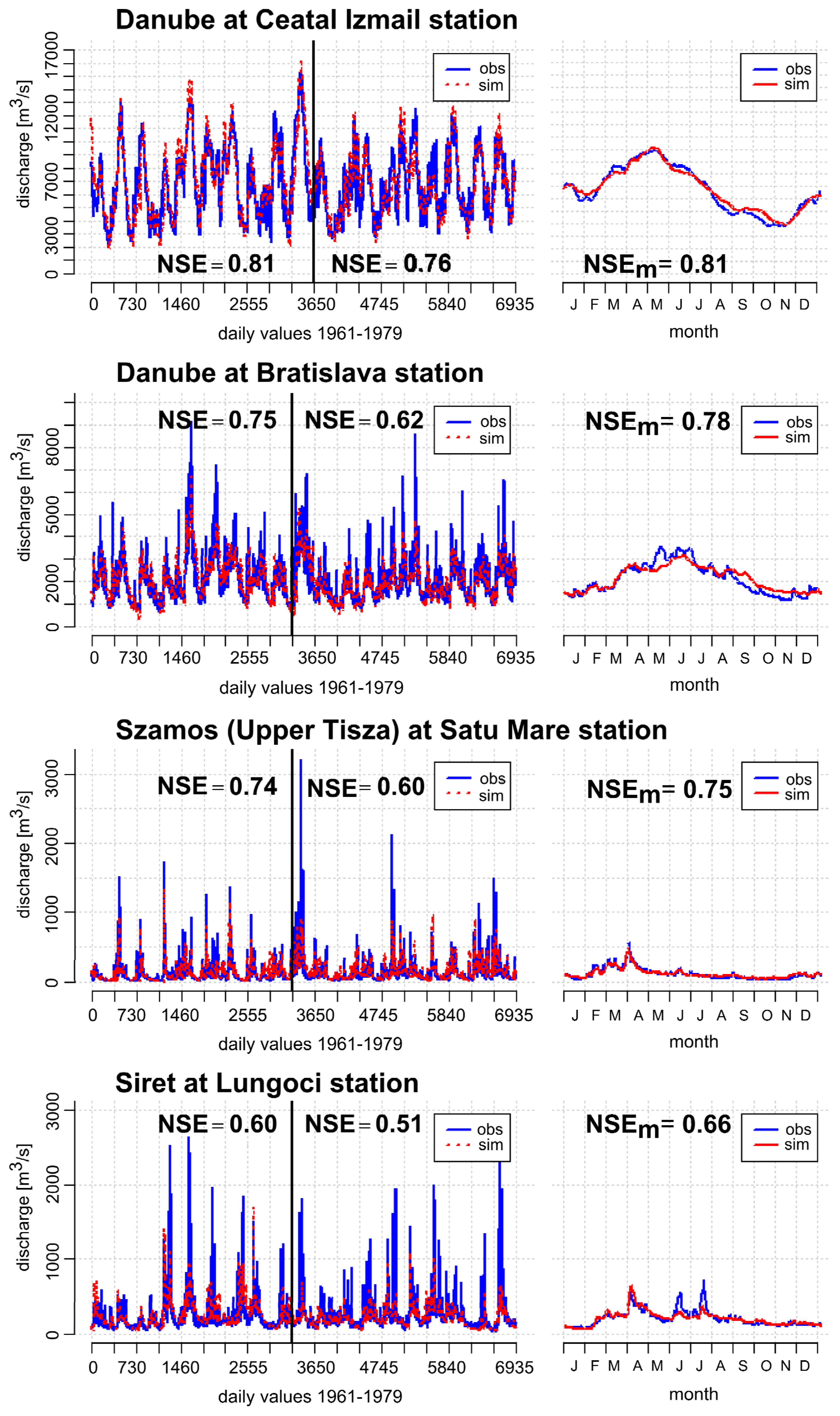
3.2.2. Model Setup, Calibration and Validation

For this study, the SWIM model was applied for the entire Danube River catchment, considering 1224 subbasins and 30,807 hydrotopes. The Danubian basin is climatically heterogeneous and characterized by a changing-complex river runoff regime varying from nival regimes in the alpine parts to mainly rain-fed regimes in the lowlands. To account for the climatically-heterogeneous river regimes of the Danubian tributaries, the SWIM model was calibrated on the basis of historic runoff data separately for 24 major river subbasins to adapt the model to the regional conditions (see Figure 7, Table 1). In particular, parameters for snow melt and sky emissivity correction, as well as the routing coefficients to calculate the storage constants for the reach and the return flow travel time have been auto-calibrated within the appropriate ranges. Additionally, Manning’s roughness coefficients have been adjusted especially in flat areas.

Figure 7. Danube catchment and the 24 selected gauging stations (see Table 2).

Figure 7. Danube catchment and the 24 selected gauging stations (see Table 2).

Table 1. Gauging stations for calibration and validation of the model. NSE, Nash–Sutcliffe model efficiency. Calibr., Calibration. Valid., Validation.

No.	Danube Basin	River	Station	Calibr. NSE	Valid. NSE	Valid. NSEm
1	Upper	Lech	Augsburg	0.50	0.43	0.49
2	Upper	Isar	Landau	0.63	0.60	0.69
3	Upper	Inn	Wasserburg	0.63	0.64	0.72
4	Upper	Salzach	Burghausen	0.64	0.58	0.74
5	Upper	Inn	Passau Ingling	0.71	0.64	0.75
6	Upper	Danube	Achleiten	0.77	0.69	0.78
7	Upper	Enns	Steyr	0.53	0.43	0.63
8	Upper	Morava	Moravsky Jan	0.74	0.72	0.79
9	Upper	Danube	Bratislava	0.75	0.62	0.78
10	Middle	Vah	Sala	0.55	0.34	0.56
11	Middle	Mur	Gornja Radgona	0.50	0.49	0.67
12	Middle	Drava	Borl	0.44	0.41	0.50
13	Middle	Szamos	Satu Mare	0.74	0.60	0.75
14	Middle	Tisza	Tiszabecs	0.45	0.42	0.56
15	Middle	Maros	Arad	0.67	0.67	0.82
16	Middle	Tisza	Szeged	0.59	0.54	0.61
17	Middle	Sava	Catez I	0.67	0.68	0.86
18	Middle	Una	Bosanski Novi	0.66	0.65	0.80
19	Middle	Sava	Sremska Mitrovica	0.81	0.77	0.83
20	Middle	Velika Morava	Lubicevsky Most	0.73	0.66	0.80
21	Middle	Danube	Bazias	0.77	0.74	0.84
22	Lower	Olt	Cornet	0.57	0.48	0.53
23	Lower	Siret	Lungoci	0.60	0.51	0.66
24	Lower	Danube	Ceatal Izmail	0.81	0.76	0.81

Table 1. Gauging stations for calibration and validation of the model. NSE, Nash–Sutcliffe model efficiency. Calibr., Calibration. Valid., Validation.

No.	Danube Basin	River	Station	Calibr. NSE	Valid. NSE	Valid. NSEm
1	Upper	Lech	Augsburg	0.50	0.43	0.49
2	Upper	Isar	Landau	0.63	0.60	0.69
3	Upper	Inn	Wasserburg	0.63	0.64	0.72
4	Upper	Salzach	Burghausen	0.64	0.58	0.74
5	Upper	Inn	Passau Ingling	0.71	0.64	0.75
6	Upper	Danube	Achleiten	0.77	0.69	0.78
7	Upper	Enns	Steyr	0.53	0.43	0.63
8	Upper	Morava	Moravsky Jan	0.74	0.72	0.79
9	Upper	Danube	Bratislava	0.75	0.62	0.78
10	Middle	Vah	Sala	0.55	0.34	0.56
11	Middle	Mur	Gornja Radgona	0.50	0.49	0.67
12	Middle	Drava	Borl	0.44	0.41	0.50
13	Middle	Szamos	Satu Mare	0.74	0.60	0.75
14	Middle	Tisza	Tiszabecs	0.45	0.42	0.56
15	Middle	Maros	Arad	0.67	0.67	0.82
16	Middle	Tisza	Szeged	0.59	0.54	0.61
17	Middle	Sava	Catez I	0.67	0.68	0.86
18	Middle	Una	Bosanski Novi	0.66	0.65	0.80
19	Middle	Sava	Sremska Mitrovica	0.81	0.77	0.83
20	Middle	Velika Morava	Lubicevsky Most	0.73	0.66	0.80
21	Middle	Danube	Bazias	0.77	0.74	0.84
22	Lower	Olt	Cornet	0.57	0.48	0.53
23	Lower	Siret	Lungoci	0.60	0.51	0.66
24	Lower	Danube	Ceatal Izmail	0.81	0.76	0.81

To assess the general predictive power of the SWIM model, the simulated river runoff was compared to the observed runoff at 24 gauging stations on a daily basis by the use of the Nash–Sutcliffe model efficiency (NSE) coefficient (see Table 1). The validation period was chosen independently from the calibration period, with at least 7 years.

The SWIM model reproduces well to very well the observed daily runoff at the different river catchments (Table 2). Most of the gauges used for calibration and validation show results >0.6 NSE on a daily basis and >0.7 NSE for monthly values [48]. For the main stations of the Danube River, the results are “good” to “very good” with a monthly NSE above 0.78 [48]. To illustrate the performance of the hydrological model, selected examples are shown in Figure 7. The model is mostly able to reproduce the monthly seasonality. For the Danube outlet at Ceatal Izmail station, the model was validated monthly with an NSE of 0.81 and a percent bias (PBIAS) of 0%. Problems appear in some headwater catchments due to less reliable meteorological input data and human interventions. For example, the seasonality of the Tisza River headwater catchment at Satu Mare is represented very well, including the snow melt-driven runoff peak in spring (Figure 8). This spring peak in runoff also fits for the Siret River (Eastern Carpathians) (Figure 8), while the pluvial summer peak could not be simulated, as these precipitation events are not in the historic (WATCH) climate data in this particular region.

3.3. Approach of the Analysis

For the projection of stream flow, we used 14 non-bias-corrected regional climate models (ENSEMBLES) as well as bias-corrected model output from 5 GCMs under different RCPs (ISI-MIP) as a daily climate driver for SWIM. For both climate scenario sets, we evaluated the relative changes in runoff between reference and future scenario periods to evaluate the climate change signals for each climate model run. The reference period is 1971–2000; the first scenario period is 2031–2060; and the second scenario period is 2071–2100. For maps, we chose to use the ensemble mean values. The ensemble mean of different climate models was found to perform better than the individual models in terms of systematic bias and produces more representative results than single RCMs [23,49,50]. In addition, the mean model tends have a similar quality for most areas and are less prone to featuring large deviations in particular areas [23].

Table 2. Changes in seasonal river runoff in (%) under two multi-model sets relative to the reference period 1971–2000 for different river stations and the scenario periods 2031–2060 and 2070–2100. The changes are shown for the winter (December to February, DJF), spring (March to May, MAM), summer (June to August, JJA) and autumn (September to November, SON) months. The ENSEMBLES projections relate to the same global warming level as the ISI-MIP 6.0.

Near Future (2031–2060)													Far Future (2070–2100)
∆ (%)	ENSEMBLES			ISI-MIP 2.6			ISI-MIP 6.0			ISI-MIP 8.5			ENSEMBLES
	min	median	max	min	median	max	min	median	max	min	median	max	min	median	max
Upper Danube River Station Bratislava
DJF	−8	21	45	−5	7	25	−2	13	31	−2	11	27	6	33	58
MAM	−9	6	23	−18	−12	−4	−13	−10	−3	−17	−10	−2	1	17	34
JJA	−21	−9	4	−17	−10	−1	−17	−10	2	−23	−13	−5	−32	−11	5
SON	−27	−1	21	−26	−6	1	−14	1	6	−32	−5	6	−48	−3	23
Middle Danube River Station Bazias (before Iron Gate)
DJF	−3	14	46	−11	−2	12	−13	−3	21	−18	−3	14	−3	28	116
MAM	−12	2	30	−22	−14	−5	−20	−9	−4	−20	−15	−7	−11	10	31
JJA	−20	−9	3	−21	−13	4	−21	−12	0	−26	−16	−11	−47	−10	10
SON	−30	−5	18	−33	−13	−1	−22	−9	2	−41	−19	−5	−49	−9	38
Lower Danube River Station Ceatal Izmail
DJF	−8	9	43	−19	−5	8	−14	−6	21	−23	−9	11	−14	24	124
MAM	−8	4	35	−22	−13	−4	−19	−9	−2	−18	−14	−8	−8	12	39
JJA	−21	−9	5	−24	−15	4	−24	−13	−4	−26	−19	−13	−49	−11	11
SON	−29	−10	11	−36	−16	−2	−25	−13	1	−44	−22	−11	−49	−12	23
Sava/Save River Station Sremska Mitrovica
DJF	−14	12	61	9	14	25	−11	15	44	−7	17	38	0	33	261
MAM	−40	−7	37	−28	−12	−5	−25	−11	−5	−33	−18	−9	−43	−13	34
JJA	−54	−26	4	−27	−18	−12	−27	−20	−6	−39	−30	−20	−72	−38	−1
SON	−58	−19	22	−33	−21	−11	−34	−11	−2	−49	−27	−10	−71	−26	42
Tisza river station Szeged
DJF	−2	16	72	−23	−6	14	−17	−7	20	−31	−13	10	1	29	248
MAM	−24	−1	55	−33	−22	−10	−33	−19	−5	−31	−26	−15	−30	3	32
JJA	−28	−10	15	−27	−16	26	−33	−7	0	−33	−21	−9	−69	−17	16
SON	−40	−7	34	−50	−18	7	−43	−26	9	−60	−39	−3	−49	−12	110

Table 2. Changes in seasonal river runoff in (%) under two multi-model sets relative to the reference period 1971–2000 for different river stations and the scenario periods 2031–2060 and 2070–2100. The changes are shown for the winter (December to February, DJF), spring (March to May, MAM), summer (June to August, JJA) and autumn (September to November, SON) months. The ENSEMBLES projections relate to the same global warming level as the ISI-MIP 6.0.

Near Future (2031–2060)													Far Future (2070–2100)
∆ (%)	ENSEMBLES			ISI-MIP 2.6			ISI-MIP 6.0			ISI-MIP 8.5			ENSEMBLES
	min	median	max	min	median	max	min	median	max	min	median	max	min	median	max
Upper Danube River Station Bratislava
DJF	−8	21	45	−5	7	25	−2	13	31	−2	11	27	6	33	58
MAM	−9	6	23	−18	−12	−4	−13	−10	−3	−17	−10	−2	1	17	34
JJA	−21	−9	4	−17	−10	−1	−17	−10	2	−23	−13	−5	−32	−11	5
SON	−27	−1	21	−26	−6	1	−14	1	6	−32	−5	6	−48	−3	23
Middle Danube River Station Bazias (before Iron Gate)
DJF	−3	14	46	−11	−2	12	−13	−3	21	−18	−3	14	−3	28	116
MAM	−12	2	30	−22	−14	−5	−20	−9	−4	−20	−15	−7	−11	10	31
JJA	−20	−9	3	−21	−13	4	−21	−12	0	−26	−16	−11	−47	−10	10
SON	−30	−5	18	−33	−13	−1	−22	−9	2	−41	−19	−5	−49	−9	38
Lower Danube River Station Ceatal Izmail
DJF	−8	9	43	−19	−5	8	−14	−6	21	−23	−9	11	−14	24	124
MAM	−8	4	35	−22	−13	−4	−19	−9	−2	−18	−14	−8	−8	12	39
JJA	−21	−9	5	−24	−15	4	−24	−13	−4	−26	−19	−13	−49	−11	11
SON	−29	−10	11	−36	−16	−2	−25	−13	1	−44	−22	−11	−49	−12	23
Sava/Save River Station Sremska Mitrovica
DJF	−14	12	61	9	14	25	−11	15	44	−7	17	38	0	33	261
MAM	−40	−7	37	−28	−12	−5	−25	−11	−5	−33	−18	−9	−43	−13	34
JJA	−54	−26	4	−27	−18	−12	−27	−20	−6	−39	−30	−20	−72	−38	−1
SON	−58	−19	22	−33	−21	−11	−34	−11	−2	−49	−27	−10	−71	−26	42
Tisza river station Szeged
DJF	−2	16	72	−23	−6	14	−17	−7	20	−31	−13	10	1	29	248
MAM	−24	−1	55	−33	−22	−10	−33	−19	−5	−31	−26	−15	−30	3	32
JJA	−28	−10	15	−27	−16	26	−33	−7	0	−33	−21	−9	−69	−17	16
SON	−40	−7	34	−50	−18	7	−43	−26	9	−60	−39	−3	−49	−12	110

Figure 8. Results of calibration and validation for selected gauging stations under historic conditions (NSE (daily NSE), NSE_m (monthly NSE), obs (observed), sim (modeled)). Left: results of calibration (first 9 years) and validation (last 11 years); right: 10-year seasonal average.

Figure 8. Results of calibration and validation for selected gauging stations under historic conditions (NSE (daily NSE), NSE_m (monthly NSE), obs (observed), sim (modeled)). Left: results of calibration (first 9 years) and validation (last 11 years); right: 10-year seasonal average.

4. Results

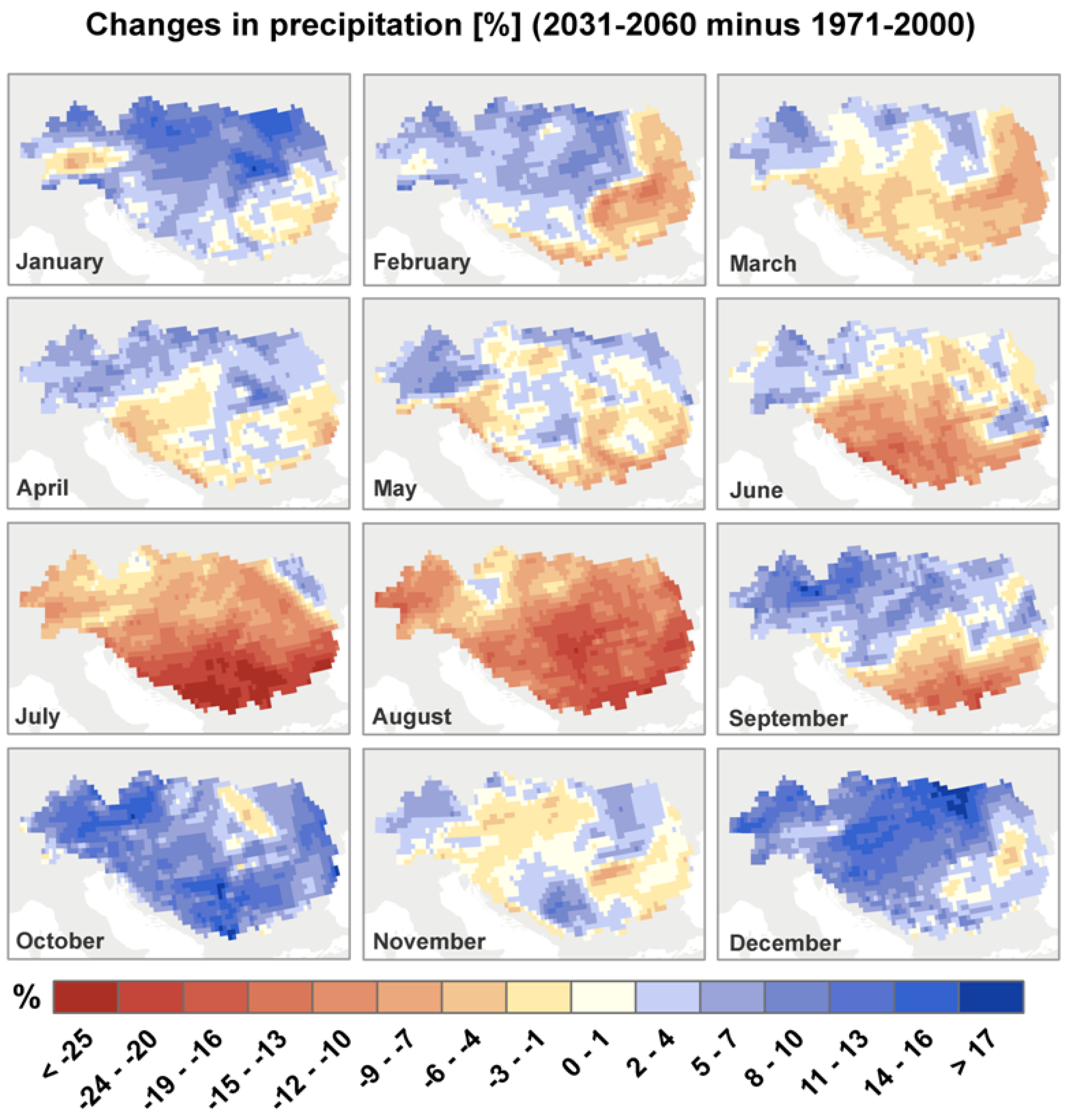
4.1. Hydro-Climatic Changes for the Whole Danube Catchment

All applied climate projections show a clear warming trend for the whole Danube basin towards the middle of the 21st century. In the summer months, the warming trend is less distinct in the Upper basin and most pronounced in the southern parts of the Lower Danube basin (more than 2 °C in the multi-model average for A1B). For precipitation, the multi-model mean (see Appendix A, Figure A1) indicates for the summer months a slight reduction in the alpine region and a stronger reduction in the Middle and Lower basin, most pronounced in the Mediterranean parts. In contrast, winter precipitation is projected to increase, mainly in the northern areas of the Danubian basin, as well as the Pannonian basin, Carpathians and the Transylvanian Plateau. A small reduction in winter precipitation is projected for the Romanian lowlands. The climatic water balance (precipitation minus potential evaporation) for the summer months indicates a reduction of water availability in the next decades all over the Danubian basin, the strongest in the Pannonian basin, the Carpathians and the Transylvanian Plateau, as well as the Mediterranean parts of the Western Balkans. For the climatic water balance, a higher surplus is projected in the winter months, except in the Lower basin, where a slight reduction becomes visible.

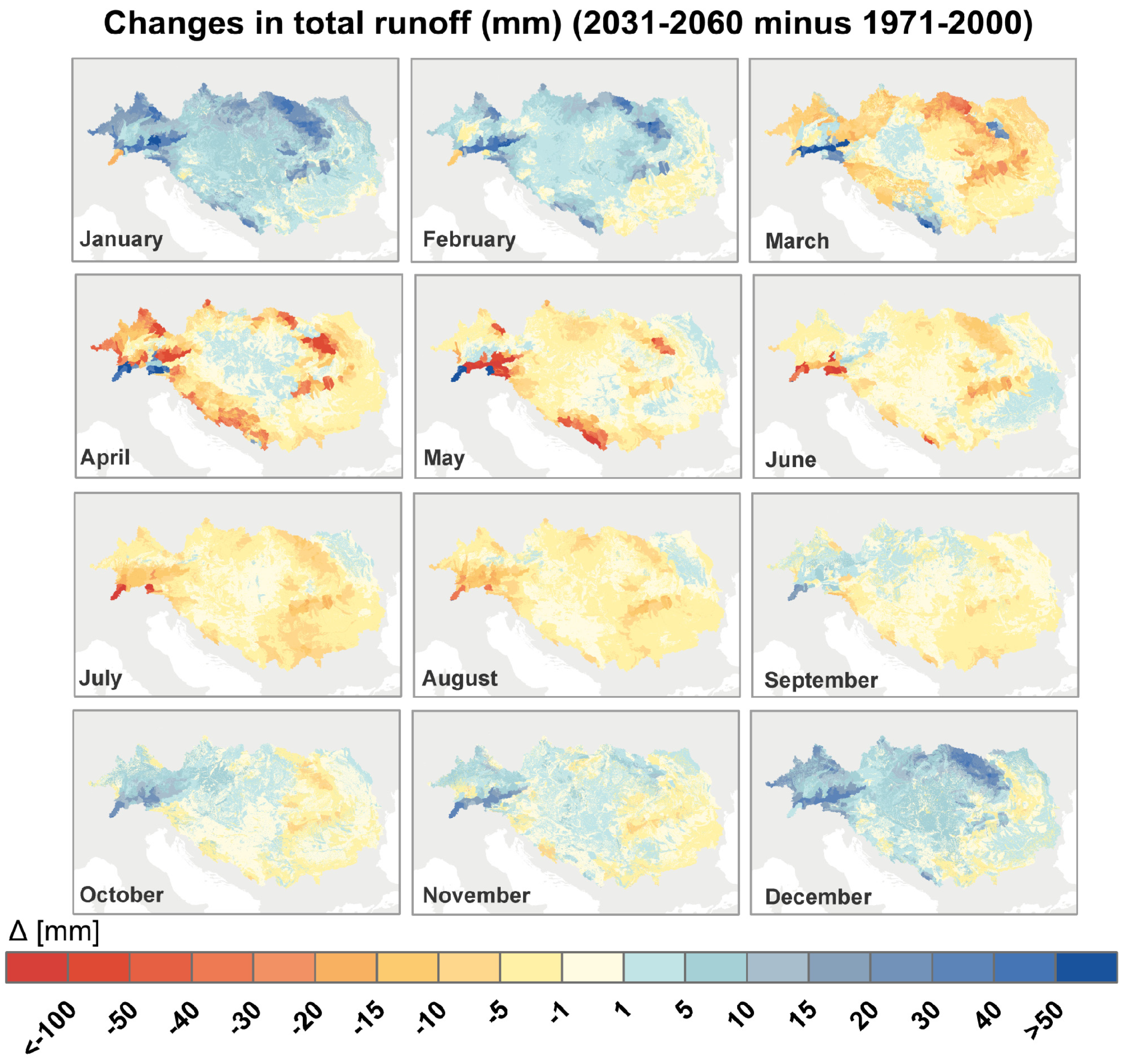
4.2. Spatial Changes in Total Runoff for the Whole Danube Basin

Maps showing the simulated total runoff (surface and subsurface runoff) have been analyzed at the hydrotope level for each month of the year, showing the differences in the scenario period 2031–2060 compared to the reference period 1971–2000 (Figure 9). The maps give the multi-model mean value of the ENSEMBLES models.

Winter (December to February): The ensemble mean shows a clear increase (10–15 mm) in mean winter runoff for nearly all parts of the basin, mainly driven by a greater amount of winter precipitation and a smaller fraction stored in snow. Winter runoff is projected to increase particularly in the Upper Danube basin and the northern Carpathians (20 mm–40 mm). Higher runoff rates can especially be found in the mountain regions induced by a rise in the snowfall lines. A decrease (<10 mm) in winter runoff (January and February) is simulated in the high mountain headwater catchment of the Inn River, where the increased precipitation is stored in ice and snow (later leading to increased runoff in April and May). Little changes in winter runoff are modeled for the Romanian-Bulgarian Lowlands in the Lower basin.

Spring (March to May): For the months of March, April and May, the ensemble mean reveals a diverse picture for changes in runoff. Despite increasing precipitation, the maps indicate a decrease in mean runoff, which is most distinct in the upper Danube basin, the Dinaric Alps and parts of the Carpathian Mountains, due to an earlier and, in part, less intense snow melt season. For April, a slight increase (<5 mm) in runoff in the Pannonian plains (Hungary) is visible. Generally, the spread in the ensemble simulations for the spring months as a transitional period gives in part different directions of runoff changes, which are hidden through the ensemble mean (see Section 4.3).

Figure 9. Changes in total runoff (mm/month) as the multi-model mean with ENSEMBLES climate data as the input; compared are the periods 1971–2000 and 2031–2060.

Figure 9. Changes in total runoff (mm/month) as the multi-model mean with ENSEMBLES climate data as the input; compared are the periods 1971–2000 and 2031–2060.

Summer (June to August): For the summer months, a general reduction in mean runoff is simulated for the entire basin due to higher temperatures leading to a higher evaporative demand and less precipitation in parts. The projected decrease in runoff is most distinct in the mountainous regions (<20 mm), mainly in the Alps, the Dinaric Alps and the Carpathians. Around the middle of the 21st century, glacier runoff contributions (mainly Inn River headwaters) are projected to decrease significantly. In contrast, the ensemble mean reveals a slight increase (<10 mm) in runoff for the Prut River Basin (Moldavia and northeastern Romania) due to increasing precipitation in this area.

Autumn (September to November): For autumn, the projected changes in runoff are divided between an increase in the northwestern parts (Upper Danube basin and Tisza basin) and a slight decrease (<5 mm) in the southeastern parts of the Danube basin. From September–November, the transition from dryer summer to wetter winter conditions gradually becomes visible. In the Mediterranean parts, the Dinaric Alps and the Carpathians, some areas show ensemble mean values with decreases up to 15 mm. The highest increase in runoff appears in the high mountain parts of the Alps (up to 30 mm). Similar to spring, the ensemble results for autumn as a transition period are partly spread in opposite directions, a fact that is hidden by the multi-model mean value.

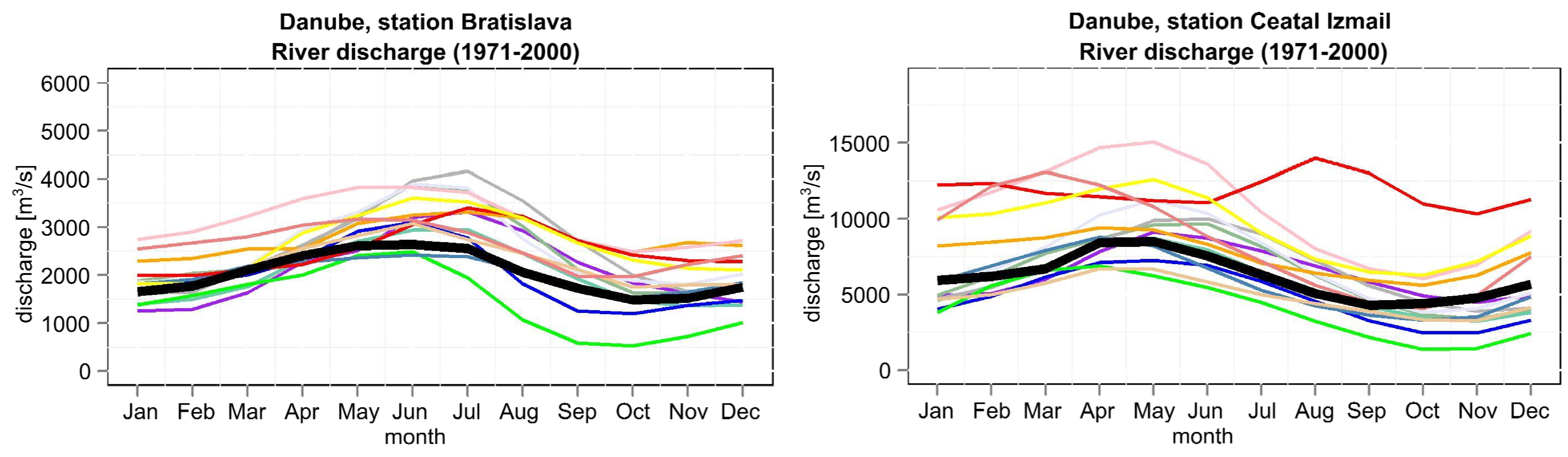
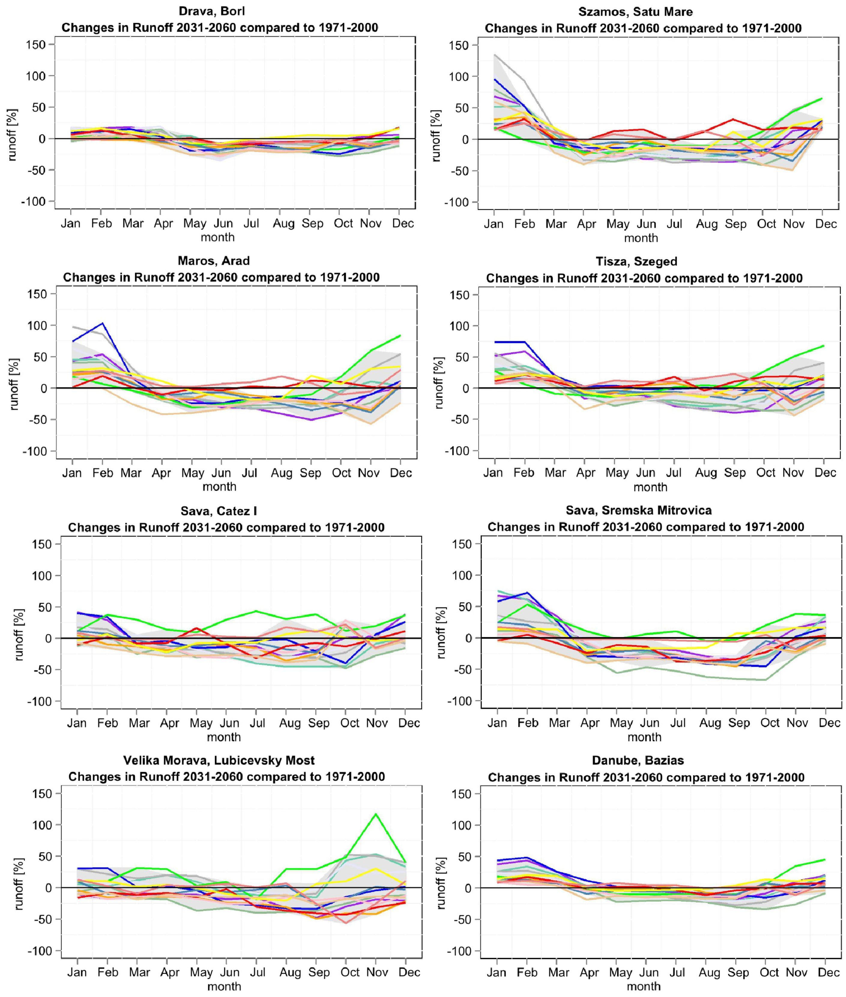
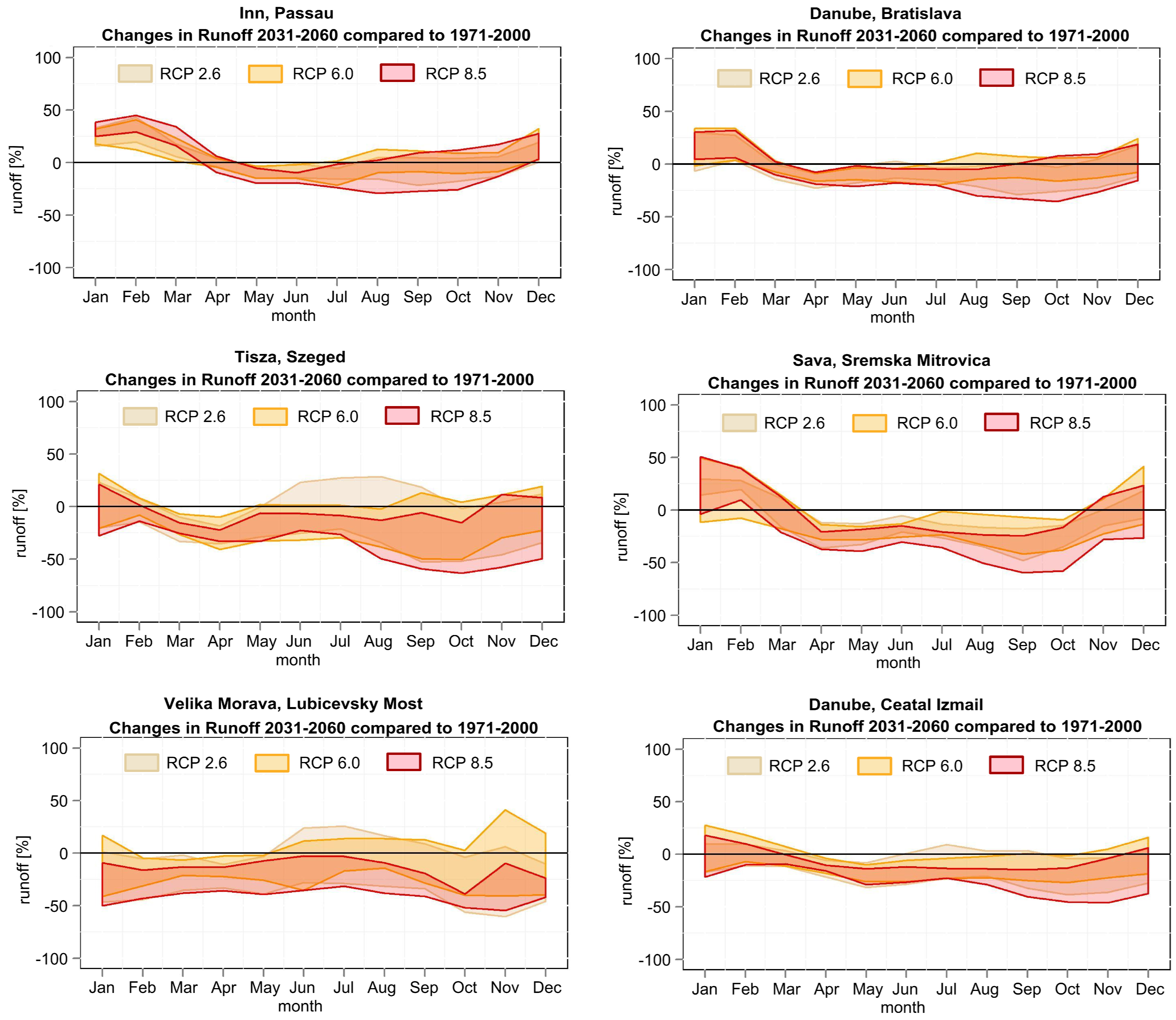
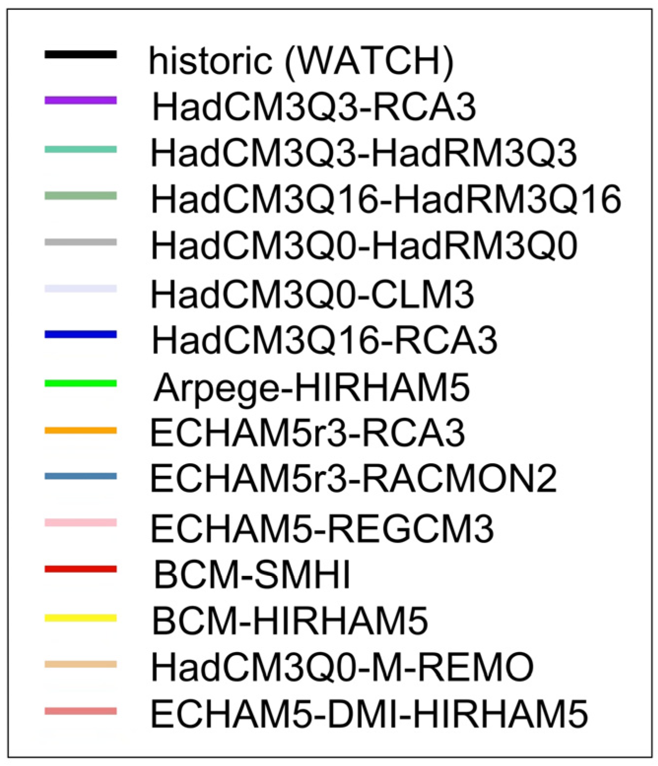
4.3. Runoff Projections for Selected River Stations

From the results for the 1224 simulated subbasins for the whole Danube, changes in the intra-annual seasonality for a selection of runoff stations are presented for the near future scenario period (years 2031–2060) and for selected stations for the far future scenario period (years 2070–2100). To bring out the underlying trends in the ensemble simulations in the graphs, a grey ribbon highlights the scenario range, excluding the outliers. Outliers are defined by the interquartile range of (Q₂₅ − 1.5 * IQR) > × > (Q₇₅ + 1.5 * IQR), with Q₂₅ = 25th percentile, IQR = interquartile range and Q₇₅ = 75th percentile.

Table 2 gives the first overview of the results for five main stations in the Danube basin for the evaluated two multi-model sets and time periods. The modeling results are presented in detail for a broad range of runoff stations in the next sections.

4.3.1. Upper Danube Basin: Snow-Rain Regime of the Alps (ENSEMBLES)

For the Upper Danube River and its tributaries, the ensemble analysis reveals a shift in runoff seasonality until the middle of this century with an increase in winter runoff and a decrease in summer runoff. Despite existing uncertainties, these trends are visible across all of the driving climate models (Figure 10). For the transition periods April, May (partially), October and November, the models do not give a clear direction. Winter runoff increases due to higher winter precipitation, as well as due to a larger fraction of precipitation falling as rain instead of snow. Additionally, snowmelt is projected to start earlier because of higher spring temperatures. The decrease in mean summer runoff is mainly due to higher evaporation rates, which cannot even be compensated by a locally small increase in summer precipitation in some areas. Moreover, in some parts of the alpine region, a decrease in precipitation is projected for summer.

The Salzach, Inn and Enns rivers (Figure 10) are representative for the alpine tributaries. From December–March, the ensemble clearly shows an increase in mean monthly runoff (20%–70%) and a decrease (2%–30%) for June–September. The projections for the Morava River, which originates in the Eastern Sudetes highlands, agree on an increasing runoff trend from October–March, but show no clear signal for the summer months.

For the Danube at gauge Bratislava (Figure 10, Table 2), which marks the end of the Upper Danube basin, the overall trends are clearly visible, but appear as a smoothed runoff curve. From May to August, the climate scenarios project a progressive decrease of up to 25% of the present runoff. From October to February, the climate scenarios show an increase in winter runoff (5%–50%).

Figure 10. Changes (%) in the mean runoff seasonality between the reference period 1971–2000 and the near future scenario period 2031–2060 for selected stations in the Upper Danube River catchment. The grey ribbon comprises the range of results without outliers.

Figure 10. Changes (%) in the mean runoff seasonality between the reference period 1971–2000 and the near future scenario period 2031–2060 for selected stations in the Upper Danube River catchment. The grey ribbon comprises the range of results without outliers.

4.3.2. Middle Danube River Basin Including Tisza and Save Rivers (ENSEMBLES)

A general reduction in summer runoff is projected across all of the models for the Middle Danube basin (Figure 11). The trends in seasonal runoff in the Middle basin are, in parts, less pronounced than in the Upper Danube basin (Figure 11). The main reasons for that is that the precipitation trends in the climate models show more disagreement for the Middle and Lower basin [22] and that snow processes, which exhibit clear trends, play a minor role outside the mountainous regions.

Figure 11. Changes (%) in the mean runoff seasonality between the reference period 1971–2000 and the near future scenario period 2031–2060 for selected stations in the Middle Danube River catchment. The grey ribbon comprises the range of results without outliers.

Figure 11. Changes (%) in the mean runoff seasonality between the reference period 1971–2000 and the near future scenario period 2031–2060 for selected stations in the Middle Danube River catchment. The grey ribbon comprises the range of results without outliers.

For the Drava headwater (Borl station), the projections show an increase (<20%) in mean runoff during the low flow season in January and February. The high flow peak in May and June caused by the alpine snow melt is projected to diminish (8%–34%) until 2060.

For the Tisza River (here represented by its headwater river Szamos, its major tributary Maros and the Tisza River station Szeged at its lower course (Table 2)), the results indicate an (up to 40%) reduced discharge peak in April–May and an earlier snow melt period. For winter runoff, particularly in January and February, a strong increase is visible (5%–50% at Szeged station) and is even more distinct in the mountain regions (10%–100%). Less river runoff is projected to aggravate the low flows in late summer and autumn.

For the alpine headwaters of the Sava River (e.g., Catez I station), as well as its tributaries originating in the Dinares, the scenarios indicate a reduction (up to ~40%) in mean river runoff from March to September, but no clear trend for late autumn and winter runoff. For the Sava River at its lower course (Sremska Mitrovica station) (Figure 11, Table 2), the modeling results indicate a further decrease (~30%) in river runoff in the low flow season from June–October and a general reduction in late spring and summer flows (up to 40%). In contrast, the modelling results show an increase in winter runoff (DJF).

The modeling results for the Velika Morava, which is dominated by a continental climate, show robust results for June–September with less runoff (up to 40%) during the low flow summer season. For the rest of the year, the models do not agree on a clear trend.

For the Danube River at Bazias station (before the Iron Gate) (Figure 11, Table 2), the modeling results project a reduction in mean runoff from May–September, up to 20%, and an increase in winter and early spring runoff (December–March) up to 40%.

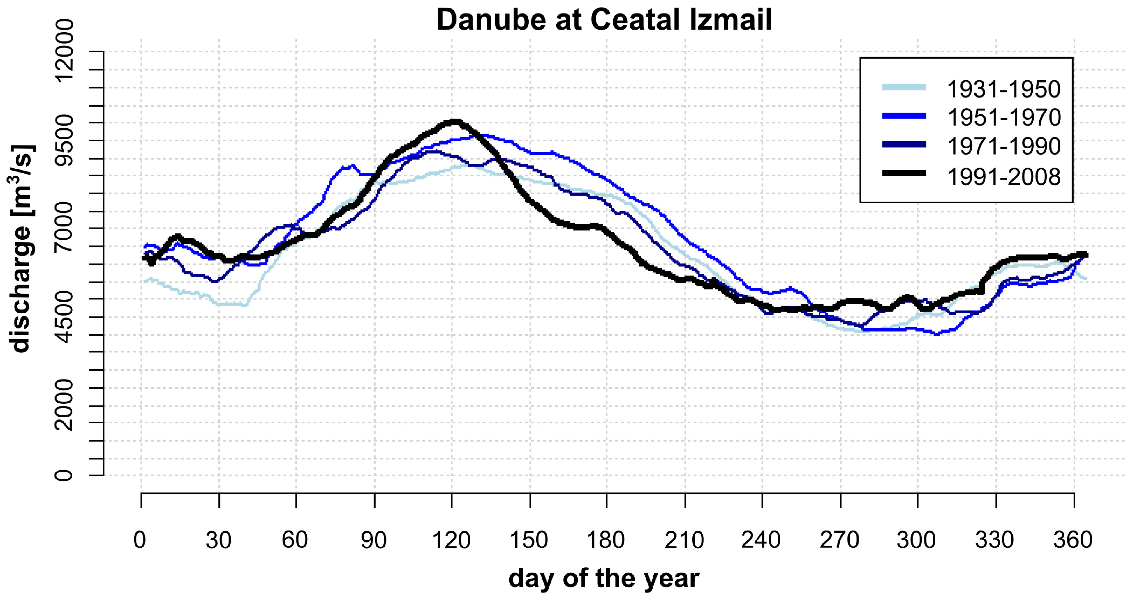
4.3.3. Lower Danube River Basin (ENSEMBLES)

For the tributaries of the Lower Danube basin, the scenario trends are partially unclear, in particular for the winter months (Figure 12). Nevertheless, the majority of the climate scenarios show a clear reduction in summer runoff, such as that for the Olt River runoff station Cornet in the southern Carpathians from March–August (up to 25%). For the Siret River, rising in the eastern Carpathians (Romania/Ukraine), a reduction in mean runoff from April–September (up to 25%) is projected, with tendencies towards an increase in mean runoff in January and February.

For the Danube River at the entrance to its delta (Ceatal Izmail station) (Figure 12, Table 2), the projections show an increase (5%–40%) in winter and early spring runoff from January–March (Figure 12). The ensemble also agrees on a decrease in river runoff in the Danubian for the summer half-year (May–October) up to 20%, aggravating the low flow season (August–November). The historical runoff peak in May is projected to decrease slightly (Ø-5%) and tends to appear earlier (April).

Figure 12. Changes (%) in the mean runoff seasonality between the reference period 1971–2000 and the near future scenario period 2031–2060 for selected stations in the Lower Danube River catchment. The grey ribbon comprises the range of results without outliers.

Figure 12. Changes (%) in the mean runoff seasonality between the reference period 1971–2000 and the near future scenario period 2031–2060 for selected stations in the Lower Danube River catchment. The grey ribbon comprises the range of results without outliers.

4.3.4. Looking ahead to the End of the 21st Century (ENSEMBLES)

The ENSEMBLES scenarios have been additionally evaluated for the far future scenario period 2071–2100 compared to the reference period 1971–2000 (Figure 13 and Table 2). For the selected runoff stations, the robust trends for the near future become more pronounced in the far future, especially for the snow-influenced ones.

For the Inn River station Passau, the scenarios for the far future show a greater increase in winter runoff and a stronger reduction in summer runoff compared to the projections for the middle of the 21st century (Figure 13). While the winter runoff is projected to increase much more, for summer runoff, the reduction in the mean monthly flows is just a little more pronounced.

For the Danube River station Bratislava, the climate change signal also becomes clearer until the end of the 21st century. The increase in winter runoff becomes more distinct in the far future scenario period, and all models agree on a reduction in runoff in August and September.

For the Tisza River station Szeged, the far future projections reveal similar trends as those for the near future for the extent of increase in winter runoff. For the rest of the year, the far future projections show a wider range in the simulations.

For the Sava River station Sremska Mitrovica, the projections for the far future show a clearer picture than those for the near future. All models agree on a reduction in monthly river flows for July–September and an increase in January and February, but the rate of the projected changes stays nearly the same.

For the Velika Morava River station Lubicevsky Most, the far future simulations show a clearer picture for the reduction in late spring and summer average river flows.

Figure 13. Changes (%) in the mean runoff seasonality between the reference period 1971–2000 and the far future scenario period 2071–2100 for selected stations in the Danube River catchment driven by the ENSEMLBES scenarios. The grey ribbon comprises the range of results without outliers.

Figure 13. Changes (%) in the mean runoff seasonality between the reference period 1971–2000 and the far future scenario period 2071–2100 for selected stations in the Danube River catchment driven by the ENSEMLBES scenarios. The grey ribbon comprises the range of results without outliers.

For the Danube River outlet at Ceatal Izmail station, the simulations for the far future reveal a border range of uncertainty. The models agree on a projected increase in runoff for January–April, while the extent of changes in winter runoff stays nearly the same as that for the mid-21st century. For the rest of the year, there is no clear picture in the changes, except for a tendency towards a decrease in late summer (Figure 13).

4.3.5. ISI-MIP Scenarios for Selected River Stations

In addition to the ENSEMBLES climate scenarios, the ISI-MIP climate scenarios have been evaluated for the near future period (Figure 14 and Table 2 for major stations). Three ISI-MIP scenarios have been selected which refer to a 2031–2060 global warming level compared to that preindustrially (1850–1900) of approximately 1.5 °C (RCP2.6), 2 °C (RCP6.0) and 2.5 °C (RCP8.5). The ENSEMBLES data under A1B SRES refer to a global warming level compared to that preindustrially (1850–1900) of +2 °C for 2031–2060, as does the ISI-MIP RCP6.0 scenario.

Figure 14. Changes (%) in the mean runoff seasonality between the reference period 1971–2000 and the near future scenario period 2031–2060 for selected stations in the Danube River catchment driven by ISI-MIP scenarios showing the range of five GCMs for each RCP (RCP2.6, RCP6.0 and RCP8.5). The ISI-MIP scenarios refer to a global warming level compared to that preindustrially (1850–1900) until 2071–2100 of 2 °C (RCP2.6), 3 °C (RCP6.0) and 4 °C (RCP8.5).

Figure 14. Changes (%) in the mean runoff seasonality between the reference period 1971–2000 and the near future scenario period 2031–2060 for selected stations in the Danube River catchment driven by ISI-MIP scenarios showing the range of five GCMs for each RCP (RCP2.6, RCP6.0 and RCP8.5). The ISI-MIP scenarios refer to a global warming level compared to that preindustrially (1850–1900) until 2071–2100 of 2 °C (RCP2.6), 3 °C (RCP6.0) and 4 °C (RCP8.5).

The evaluation of changes in seasonal runoff for the near future scenario period 2031–2060 shows very similar patterns for the RCP6.0 compared to the ENSEMLBES models under SRES A1B. In most cases, the bias-corrected ISI-MIPs range within the ENSEMBLES results, but due to the lower number of scenario runs and due to bias correction, they show a smaller range of uncertainty than the ENSEMBLES models. For all selected runoff stations, the “warmest scenario” RCP8.5 reveals a clear reduction in river runoff for the summer months.

For the Upper Danube River stations Inn at Passau and Danube at Bratislava, the patterns are very similar to the results from the ENSEMLBES models. In the RCP8.5 scenario, the projected trends of an increase in winter runoff and reduction in the summer months become more pronounced.

For the Tisza River station Szeged, the ISI-MIP RCP6.0 shows patterns similar to the ENSEMLBES models for summer runoff. However, while all of the ENSEMBLES models show a runoff increase for the winter months, the ISI-MIPs reveal no clear signal and a higher range of uncertainty (and even a tendency for reduction in winter).

For the Sava River station Sremska Mitrovica, ENSEMBLES and ISI-MIPs show quite similar patterns for seasonal runoff changes, through the ISI-MIPs’ reduction signal for summer and autumn runoff is more distinct.

For the Velika Morava River station Lubicevsky Most, the ENSEMBLES models do not show clear trends for most of the year, but tend towards a reduction in average summer runoff. The ISI-MIPs agree on a reduction in spring runoff, while the ENSEMBLES do not give a clear picture for the same period. For the highest ISI-MIP warming scenario (RCP8.5), a clear decrease in monthly mean runoff for the entire year is projected.

For the Danube outlet station Ceatal Izmail, the ISI-MIP scenarios do not give a clear trend from January–March, while the ENSEMBLES have projected an increase in average river runoff for the same time period (Figure 14). The trend towards a reduction in summer is much more distinct than under the ENSEMBLES scenarios, especially for the higher-end scenarios. ISI-MIP scenarios for RCP8.5 project a clear reduction in monthly river runoff from spring to autumn.

5. Discussion

5.1. Changes in Streamflow Seasonality under Climate Change

In this study, we investigated the potential impacts of climate change on the seasonal runoff regime of the Danube River and its tributaries. Uncertainties about future changes in the hydrological regime are generally great, but do show some robust trends. In many cases, a concise comparison of our results with previous studies is only partly feasible as the studies applied other modeling approaches on different scales, evaluated other time frames, scenarios and/or presented different indicators. As found in other studies [15], the modeling results largely depend on the underlying climate scenarios, resulting in sometimes contradictory statements in some regions about the water availability in the Danube basin.

For the Upper Danube River catchment, our results confirm the general trends found in previous studies [12,13,14,15]. For the alpine parts, our modeling results clearly show an earlier runoff peak and a shift from summer to spring due to a changed snow regime. This is in line with the climate impacts reported in Mauser et al. [15], who projected for the Upper Danube River basin a higher water availability in winter and lower water availability in summer. In the GLOWA-Danube project, the Upper Danube basin was simulated up to the station Achleiten with the hydrological model PROMET under various statistical climate trends [51]. They found similar spatial patterns in the runoff change (2036–2060 minus 1971–2000) for the Upper Danube basin with a reduction of the annual mean runoff most distinct in the alpine parts and the foothills of the Alps. For the Danube station Achleiten, GLOWA projected a reduction in annual runoff until 2060 of 9%–31% depending on the climate scenario and a shift in the annual (historical) summer maximum flows to spring [12]. In contrary, the SWIM model results exhibited only a minimal reduction (<5%) in the average annual discharge for the Danube station Achleiten (2031–2060 minus 1971–2000).

Kling et al. [13] modeled the Upper Danube catchment up to Vienna with bias-corrected ENSEMBLES scenario data. They found that the ensemble mean for 2071–2100 at Vienna results in a decrease in annual runoff by 15%. The seasonal runoff is strongly affected in summer, with a median decrease in August of 17% for 2021–2050 and 40% for 2071–2100. They also report a slight increase in winter runoff for 2071–2100, but not for 2021–2050 [13]. Our modeling results for the Danube station at Bratislava (60 km downstream of Vienna station) show a less distinct decease in summer runoff for August (−14% for 2031–2060 and −20% for 2071–2100) and no change in the annual mean runoff.

In the AdaptAlp project, the Inn River was modeled with three hydrological models driven by the ENSEMBLES climate models [52]. Similar to our results, they projected for the near future (until 2050) a clear seasonal shift with an increase in the historically much lower winter discharge and a decrease in the historically high summer discharge projections. This would mean a shift towards a more rainfall-influenced regime, though snowmelt processes are projected to still play an important role [52]. Other studies focusing on runoff contribution from glaciers [18,19] show that the ongoing glacier retreat in the future (after 2040) might lead to a shift in the runoff regime from glacial to nival for small and highly glaciated catchments [53].

For the Middle Danube basin, the few available project studies agree on an increase in runoff in winter and, apart from less future precipitation in the summer months, make some contradictory statements regarding the rest of the year [15,54]. Though our ensemble results for the middle Danube River Basin show a larger range in the direction of change outside of the winter months, the majority of the scenarios indicate a decrease in runoff from April–September. The trends become especially clear in the results for the far future and the high end climate scenarios. Within the scope of the CLAVIER (Climate Change and Variability: Impact on Central and Eastern Europe) project, climate impacts for the near future (2021–2050 compared to 1961–1990) on the Tisza River were assessed with the use of two GCMs (based on the A1B scenario) and two RCMs and the conceptual hydrological models VITUKI-NHFS and VIDRA [55]. For the Maros at Arad station, they projected a general decrease in mean annual discharges (10% to 15%), an increase in the winter season and a decrease in the mean discharges from spring to autumn (15% to 20%). Our modeling results for the Maros (Arad station) show a slighter decrease in the annual mean runoff (median ~11%), also an increase in DJF (28%) and a reduction in spring (5%) and autumn (20%) mean discharges. For the Tisza station at Szeged, the CLAVIER project simulated an increase in winter discharge (20%) and a decrease in spring and summer of 10% [55]. For the Tisza River, we simulated using the ENSEMBLES scenarios an increase in river runoff for DJF (23%), and the majority of scenarios shows a decrease in runoff from April–September. These results range near the multi-model mean values of our results (for summer, −10%), which show a broader range as more scenarios have been applied. However, for autumn, our modeling results for the Szeged station do not show a clear direction.

For the Lower Danube basin, climate impact studies are scarce. A few small-scale studies indicate a general decrease in the mean annual runoff, along with an increase of runoff in winter and a decrease in summer; the latter might lead to greater water stress in summer [15]. Our results agree on a decrease in summer runoff, especially in the 3 °C scenario, but no clear statement about the winter runoff can be issued. In the CECILIA project (Central and Eastern Europe Climate Change Impact and Vulnerability Assessment) [56], two small Romanian tributaries, the Ialomita and Buzau rivers originating in the eastern Carpathians to the north of Bucharest, have been modeled with the hydrological model WATBAL based on the RegCM climate scenario. The mean monthly flow simulations for these rivers show either no change or an increase in winter for the near future period (2021–2050) and a clear decrease in spring and summer, especially in the far future period (2071–2100). Similarly, we simulated a general runoff reduction in this area, except for December and January (see Figure 9).

5.2. Sources of Uncertainties

Uncertainties in the projection of future river flows arise from different sources in the hydro-climatic modeling chain, resulting in the broad range of projected changes. In the analysis of the impact on simulated runoff, Graham et al. [57] found, among others [58,59], that the largest source of uncertainty comes from GCM forcing, which has a greater impact on projected hydrological change than the selected RCM or the emission scenario, at least until the middle of the century. Hence, the uncertainty related to different hydrological models and their parameterization is significantly less important compared to the uncertainty resulting from a large number of climate scenarios, though the effects of hydrological model structural uncertainty on projected changes can be substantial [1,60]. Some studies (e.g., [61]) recommend that decisions and impact modeling should be based on the ensemble mean from various climate projections, such as that which we used for our maps of runoff changes. However, it is not known to what extent this can actually reduce the overall uncertainties. Furthermore, ensembles can become biased when using many different versions of similar descriptions of physical laws. As the selected climate models do not cover the whole CMIP5 spectrum, the range of the results, as well as the multi-model mean could vary if more climate scenarios are included in the study.

Generally, for the 2 °C warming scenario for 2031–2060 (A1B and RCP6.0), the bias-corrected ISI-MIP scenarios (five GCMs) are found to spread less and their results are located within the middle range compared to the ENSEMBLES climate models. The sole exception is in the Middle basin, where the ISI-MIPs do not show a clear signal for January and February (for all RCPs), while the ENSEMBLES models agree on an increase in winter runoff. This confirms previous findings that the use of bias correction methods leads to a better fit of the hydrological model output and narrows the variability bounds [62,63]. Some studies recommend applying bias correction to hydrological impact studies, even though bias correction adds significantly to the uncertainties in impact assessments [63]. Others estimate the influence of bias correction on the relative change of flow indicators between reference and future scenario periods to be weak ([9] for the same set of ENSEMBLES climate scenarios), with the exception of the timing of the spring flood peak [26]. Huang et al. [64] used bias-corrected and uncorrected climate scenarios to drive a hydrological model for the largest German river basins and came to the result that the performance of bias correction depends on the method selected, the length of the calibration period and the RCMs used. In addition, bias correction can even lead to a change in trends, especially for extremes. Bosshard et al. [62] show that choosing different methods for bias correction can increase the uncertainty of modelled river runoff substantially. Following this discussion, it can be concluded that in a study focusing on relative changes and not absolute values (of hydrological quantities), bias correction of climate input can increase the inherent uncertainty of the results while not adding much additional information.

In this study, the modeling results for runoff agreed the most for the Upper Danube basin and the least for the Lower basin (Romania), mainly because of the disagreement among the climate projections for (winter) precipitation. In Central and Eastern Europe, the uncertainty stemming from the choice of climate model was derived mainly from uncertainties in precipitation due to their location in a climatic transition zone, while the direction of the temperature trend was confirmed by all of the ENSEMBLES models [21]. Generally, precipitation patterns in climate models vary substantially for different parts of Europe (e.g., [65]). Furthermore, hydrological and meteorological measurement data for the Middle and Lower Danube basin, especially in the Balkan countries, are less available than, e.g., for the Upper Danube basin.

The present future scenarios consider changes in atmospheric concentration of climate gases. However, also, other drivers of the hydrological regime, such as land use and vegetation, river channel modifications or water management, may change in the future, which are not considered in the simulations.

6. Summary and Conclusions

With a regional hydrological model and a broad ensemble of climate scenarios, we estimated the impacts of climate change on runoff seasonality in the Danube River catchment. This study provides information about potential hydrological impacts, also for regions where no regional modeling studies have yet been carried out with an ensemble of various climate models. Despite the existing range of modelling uncertainty, some patterns show up very clearly among the simulations, which can be incorporated in applied planning measures. For the Danube River basin and its tributaries, the scenarios agree on a general trend with a distinct reduction in summer river flows and an increase in winter runoff.

The projections for the Upper Danube basin reveal a clear decrease in summer runoff from May–August, most distinct in the Alps. However, in the Middle basin (especially in the Dinaric Alps, Carpathians and Mediterranean parts), the reduction in runoff is projected to be even more pronounced and prolonged, reaching from late spring to early autumn (April–October). Especially in the Middle and Lower basin, climate change is projected to aggravate the low flows in late summer and autumn. In contrast, more river runoff is modeled in winter and early spring for most parts of the Danube basin. This is most distinct for the higher mountain catchments originating in the Alps and the Carpathians. Thus, the most pronounced increases in (winter) runoff are visible for rivers of the Upper Danube basin (December–March), followed by the Tisza River (January–March) and less distinct ones for the Sava River and some rivers in the Lower Danube basin (January and February). For the Middle and Lower basin, the climate scenarios agree less on changes in winter precipitation leading, e.g., for the Velika Morava River, to no clear direction of runoff changes.

In this study, we used a variety of non-bias-corrected and bias-corrected climate scenarios for 1.5 °C, 2 °C and 3 °C warming levels compared to the preindustrial level. The evaluation of changes in seasonal runoff for a 2 °C warming, represented here by the near future scenario period 2031–2060 in the ENSEMBLES models under A1B and the bias-corrected ISI-MIPs under the RCP6.0, shows very similar patterns. In most cases, the ISI-MIPs range within the ENSEMBLES results, but show, due to the lower number of scenario runs and the bias correction, a smaller range of uncertainty. The scenarios for a 2.5–3 °C-warming show similar trends regardless of whether the A1B scenario (ENSEMBLES) in the far future (2071–2100) or the RCP8.5 (ISI-MIPs) in the near future (2031–2060) was considered. In the higher-end climate scenarios, the trends become very distinct, particularly the decrease in water availability during the summer months. Generally, the Middle and Lower Danube basin are likely to suffer water use conflicts with accelerating climate warming.

References

1. Cisneros, J.B.E.; Oki, T.; Arnell, N.W.; Benito, G.; Cogley, J.G.; Döll, P.; Jiang, T.; Mwakalila, S.S. Freshwater resources. In Climate Change 2014: Impacts, Adaptation, and Vulnerability, Part A: Global and Sectoral Aspects; Contribution of Working Group II to the Fifth Assessment Report of the Intergovernmental Panel on Climate Change; Field, C.B., Barros, V.R., Dokken, D.J., Mach, K.J., Mastrandrea, M.D., Bilir, T.E., Chatterjee, M., Ebi, K.L., Estrada, Y.O., Genova, R.C., et al., Eds.; Cambridge University Press: Cambridge, UK; New York, NY, USA, 2014; pp. 229–269. [Google Scholar]
2. Hattermann, F.F.; Post, J.; Krysanova, V.; Conradt, T.; Wechsung, F. Assessment of water availability in a central-european river basin (Elbe) under climate change. Adv. Clim. Chang. Res. 2008, 4, 42–50. [Google Scholar]
3. Hattermann, F.F.; Kundzewicz, Z. Water Framework Directive: Model Supported Implementation: A Water Manager’s Guide; Iwa Publishing: London, UK, 2010. [Google Scholar]
4. Sommerwerk, N.; Hein, T.; Schneider-Jacoby, M.; Baumgartner, C.; Ostojic, A.; Siber, R.; Bloesch, J.; Paunovic, M.; Tockner, K. The Danube River Basin. In Rivers of Europe; Tockner, K., Robinson, C.T., Uehlinger, U., Eds.; Academic Press: Oxford, UK, 2009; pp. 59–112. [Google Scholar]
5. Nachtnebel, H.-P. The Danube river basin environmental programme: Plans and actions for a basin wide approach. Water Policy 2000, 2, 113–129. [Google Scholar] [CrossRef]
6. Giorgi, F. Climate change hot-spots. Geophys. Res. Lett. 2006, 33. [Google Scholar] [CrossRef]
7. Teutschbein, C.; Seibert, J. Regional Climate Models for Hydrological Impact Studies at the Catchment Scale: A Review of recent modeling Strategies. Geogr. Compass 2010, 4, 834–860. [Google Scholar] [CrossRef] [Green Version]
8. Aich, V.; Liersch, S.; Vetter, T.; Huang, S.; Tecklenburg, J.; Hoffmann, P.; Koch, H.; Fournet, S.; Krysanova, V.; Müller, E.N.; et al. Comparing impacts of climate change on streamflow in four large African river basins. Hydrol. Earth Syst. Sci. 2014, 18. [Google Scholar] [CrossRef]
9. Hattermann, F.F.; Huang, S.; Koch, H. Climate change impacts on hydrology and water resources. Meteorol. Z. 2015, 24. [Google Scholar] [CrossRef]
10. Giorgi, F. Uncertainties in climate change projections, from the global to the regional scale. EPJ Web Conf. 2010, 9. [Google Scholar] [CrossRef]
11. Collins, M. Ensembles and probabilities: A new era in the prediction of climate change. Philos. Trans. R. Soc. A 2007, 365. [Google Scholar] [CrossRef] [PubMed]
12. Zabel, F. Teilprojekt Hydrologie/Fernerkundung—Änderung des Wasserhaushalts im Zuge des Klimawandels, Kapitel 3.1.1. In GLOWA-Danube-Projekt, LMU München (Hrsg.): Global Change Atlas; Einzugsgebiet Obere Donau: München, Germany, 2009. [Google Scholar]
13. Kling, K.; Fuchs, M.; Paulin, M. Runoff conditions in the upper Danube basin under an ensemble of climate change scenarios. J. Hydrol. 2012, 424, 264–277. [Google Scholar] [CrossRef]
14. Szépszó, G.; Lingemann, I.; Klein, B.; Kovács, M. Impact of climate change on hydrological conditions of Rhine and Upper Danube rivers based on the results of regional climate and hydrological models. Nat. Hazards 2014, 72, 241–262. [Google Scholar] [CrossRef]
15. Mauser, W.; Prasch, M.; Koch, F.; Weidinger, R. Danube Study—Climate Change Adaptation, Danube River Basin Climate Change Adaptation. Final Project Report. p. 174. Available online: http://www.icpdr.org/main/activities-projects/climate-change-adaptation (assessed on 13 May 2013).
16. Schiller, H.; Miklós, D.; Sass, J. The Danube River and its Basin Physical Characteristics, Water Regime and Water Balance. In Hydrological Processes of the Danube River Basin; Brilly, M., Ed.; Springer Netherlands: Dordrecht, Netherland, 2010; pp. 25–78. [Google Scholar]
17. ICPDR—International Commission for the Protection of the Danube River. Map 3: Annual Precipitation. Available online: https://www.icpdr.org/main/resources/map-3-annual-precipitation (accessed on 24 September 2015).
18. Huss, M. Present and future contribution of glacier storage change to runoff from macroscale drainage basins in Europe. Water Resour. Res. 2011, 47. [Google Scholar] [CrossRef]
19. Weber, M.; Braun, L.; Mauser, W.; Prasch, M. Contribution of rain, snow- and icemelt in the upper Danube discharge today and in the future. Geogr. Fis. Dinam. Quat. 2010, 33, 221–230. [Google Scholar]
20. Zaharia, L. The Iron Gates Reservoir—Aspects concerning hydrological characteristics and water quality. Lakes Reserv. Ponds 2010, 4, 52–69. [Google Scholar]
21. Van der Linden, P.; Mitchell, J. ENSEMBLES: Climate Change and Its Impacts: Summary of Research and Results from the ENSEMBLES Project; Met Office Hadley Centre: Exeter, UK, 2009. [Google Scholar]
22. Stagl, J.; Hattermann, F.F.; Vohland, K. Exposure to climate change in Central Europe: What can be gained from regional climate projections for management decisions of protected areas? Reg. Environ. Chang. 2014, 15. [Google Scholar] [CrossRef]
23. Jacob, D.; Bärring, L.; Christensen, O.B.; Christensen, J.H.; de Castro, M.; Deque, M.; Giorgi, F.; Hagemann, S.; Hirschi, M.; Jones, R.; et al. An inter-comparison of regional climate models for Europe: Model performance in present-day climate. Clim. Chang. 2007. [Google Scholar] [CrossRef]
24. Weedon, G.P.; Gomes, S.; Viterbo, P.; Shuttleworth, W.J.; Blyth, E.; Österle, H.; Adam, J.C.; Bellouin, N.; Boucher, O.; Best, M. Creation of the WATCH forcing data and its use to assess global and regional reference crop evaporation over land during the twentieth century. J. Hydrometeorol. 2011, 12, 823–848. [Google Scholar] [CrossRef]
25. Ehret, U.; Zehe, E.; Wulfmeyer, V.; Warrach-Sagi, K.; Liebert, J. HESS Opinions “Should we apply bias correction to global and regional climate model data?”. Hydrol. Earth Syst. Sci. 2012, 16. [Google Scholar] [CrossRef]
26. Muerth, M.J.; GauvinSt-Denis, B.; Ricard, S.; Velázquez, J.A.; Schmid, J.; Minville, M.; Caya, D.; Chaumont, D.; Ludwig, R.; Turcotte, R. On the need for bias correction in regional climate scenarios to assess climate change impacts on river runoff. Hydrol. Earth Syst. Sci. 2013, 17, 1189–1204. [Google Scholar] [CrossRef]
27. Addor, N.; Seibert, J. Bias correction for hydrological impact studies-beyond the daily perspective. Hydrol. Process. 2014, 28, 4823–4828. [Google Scholar] [CrossRef]
28. Liu, M.; Rajagopalan, K.; Chung, S.H.; Jiang, X.; Harrison, J.; Nergui, T.; Guenther, A.; Miller, C.; Reyes, J.; Tague, C.; et al. What is the importance of climate model bias when projecting the impacts of climate change on land surface processes? Biogeosciences 2014, 11, 2601–2622. [Google Scholar] [CrossRef]
29. Teutschbein, C.; Seibert, J. Is bias correction of regional climate model (RCM) simulations possible for non-stationary conditions? Hydrol. Earth Syst. Sci. 2013, 17. [Google Scholar] [CrossRef]
30. Hagemann, S.; Chen, C.; Hearter, J.O.; Heinke, J.; Gerten, D.; Piani, C. Impact of a statistical bias correction on the projected hydrological changes obtained from three GCMs and two hydrological models. J. Hydrometeorol. 2011, 12. [Google Scholar] [CrossRef]
31. Déqué, M.; Rowell, D.P.; Lüthi, D.; Giorgi, F.; Christensen, J.H.; Rockel, B.; Jacob, D.; Kjellström, E.; de Castro, M.; van den Hurk, B. An intercomparison of regional climate simulations for Europe: Assessing uncertainties in model projections. Clim. Chang. 2007, 81, 53–70. [Google Scholar] [CrossRef]
32. Tebaldi, C.; Knutti, R. The use of the multi-model ensemble in probabilistic climate projections. Philos. Trans. R. Soc. A 2007, 265. [Google Scholar] [CrossRef] [PubMed]
33. Warszawski, L.; Frieler, K.; Huber, V.; Piontek, F.; Serdeczny, O.; Schewe, J. The Inter-Sectoral Impact Model Intercomparison Project (ISI-MIP): Project framework. PNAS 2013, 111, 3228–3232. [Google Scholar] [CrossRef] [PubMed]
34. Hempel, S.; Frieler, K.; Warszawski, L.; Schewe, J.; Piontek, F. A trend-preserving bias correction—The ISI-MIP approach. Earth Syst. Dynam. 2013, 4. [Google Scholar] [CrossRef]
35. Krysanova, V.; Wechsung, F.; Hattermann, F.F. Development of the ecohydrological model SWIM for regional impact studies and vulnerability assessment. Hydrol. Process. 2005, 19, 763–783. [Google Scholar] [CrossRef]
36. Hattermann, F.F.; Weiland, M.; Huang, S.; Krysanova, V.; Kundzewicz, Z.W. Model-Supported impact assessment for the water sector in Central Germany under climate change—A case study. Water Resour. Manag. 2011, 25, 3113–3134. [Google Scholar] [CrossRef]
37. Williams, J.R.; Renard, K.G.; Dyke, P.T. EPIC a new method for assessing erosion’s effect on soil productivity. J. Soil Water Conserv. 1984, 38, 381–383. [Google Scholar]
38. Huang, S.; Krysanova, V.; Hatterman, F.F. Projection of Low Flow Conditions in Germany under Climate Change by Combining Three RCMs and a Regional Hydrological Model. Acta Geophys. 2013, 61. [Google Scholar] [CrossRef]
39. Hock, R. Glacier melt: A review of processes and their modelling. Prog. Phys. Geogr. 2005, 29, 362–391. [Google Scholar] [CrossRef]
40. SRTM 90m Digital Elevation Data. Available online: http://srtm.csi.cgiar.org/ (accessed on 25 January 2011).
41. Bossard, M.; Feranec, J.; Otahel, J. CORINE Land Cover Technical Guide—Addendum 2000; EEA Technical Report European Environment Agency: Copenhagen, Denmark, 2000. [Google Scholar]
42. Lehner, B.; Liermann, C.R.; Revenga, C.; Vörösmarty, C.; Fekete, B.; Crouzet, P.; Döll, P.; Endejan, M.; Frenken, K.; Magome, J.; et al. High-resolution mapping of the world's reservoirs and dams for sustainable river-flow management. Front. Ecol. Environ. 2011, 9. [Google Scholar] [CrossRef]
43. Uppala, S.M.; Kållberg, P.W.; Simmons, A.J.; Andrae, U.; da Costa Bechtold, V.; Fiorino, M.; Gibson, J.K.; Haseler, J.; Hernandez, A.; Kelly, G.A.; et al. The ERA-40 re-analysis. Quart. J. R. Meteorol. Soc. 2005, 131. [Google Scholar] [CrossRef]
44. Mitchell, T.D.; Jones, P.D. An improved method of constructing a database of monthly climate observations and associated high-resolution grids. Int. J. Climatol. 2005, 25, 693–712. [Google Scholar] [CrossRef]
45. Weedon, G.P.; Gomes, S.; Viterbo, P.; Österle, H.; Adam, J.C.; Bellouin, N.; Boucher, O.; Best, M. The WATCH Forcing Data 1958–2001: A Meteorological Forcing Dataset for Land Surface- and Hydrological Models. WATCH Technical Report 22. 2010, p. 41. Available online: http://www.eu-watch.org/media/default.aspx/emma/org/10376311/WATCH+Technical+Report+Number+22+The+WATCH+forcing+data+1958-2001+A+meteorological+forcing+dataset+for+land+surface-+and+hydrological-models.pdf (accessed on 4 March 2013).
46. Rust, H.W.; Kruschke, T.; Dobler, A.; Fischer, M.; Ulbrich, U. Discontinuous Daily Temperatures in the WATCH Forcing Datasets. J. Hydrometeorol. 2015, 16. [Google Scholar] [CrossRef]
47. Climate Research Unit, Gridded station observations, CRU TS 2.10. Gridded Station Counts Per Variable. 2004. Available online: http://www.cru.uea.ac.uk/cru/data/hrg/cru_ts_2.10/ (accessed on 10 October 2015).
48. Moriasi, D.N.; Arnold, J.G.; van Liew, M.W.; Bingner, R.L.; Harmel, R.D.; Veith, T.L. Model evaluation guidelines for systematic quantification of accuracy in watershed simulations. Trans. Am. Soc. Agric. Biol. Eng. 2007, 50, 885–900. [Google Scholar]
49. Kyselý, J.; Gaál, L.; Beranová, R.; Plavcová, E. Climate change scenarios of precipitation extremes in Central Europe from ENSEMBLES regional climate models. Theor. Appl. Climatol. 2011, 104, 529–542. [Google Scholar] [CrossRef]
50. Kjellström, E.; Nikulin, G.; Hansson, U.; Strandberg, G.; Ullerstig, A. 21st century changes in the European climate: Uncertainties derived from an ensemble of regional climate model simulations. Tellus A 2011, 63, 24–40. [Google Scholar] [CrossRef]
51. Mauser, W.; Prasch, M. (Eds.) Regional Assessment of Global Change Impacts—The Project GLOWA-Danube; Springer International Publishing: Cham, Switzerland, 2015; p. 390.
52. AdaptAlp: Water Regime in the Alpine Space—The Inn River Basin, Adapt Alp WP4 Water Regime. Project Report. 2011, p. 28. Available online: http://www.adaptalp.org/index.php?option=com_docman&task=doc_download&gid=409&Itemid=79 (assessed on 2 March 2014).
53. Koboltschnig, G.R.; Schöner, W. The relevance of glacier melt in the water cycle of the Alps: The example of Austria. Hydrol. Earth Syst. Sci. 2011, 15. [Google Scholar] [CrossRef]
54. Lobanova, A.; Stagl, J.; Vetter, T.; Hattermann, F. Discharge Alterations of the Mures River, Romania under Ensembles of Future Climate Projections and Sequential Threats to Aquatic Ecosystem by the End of the Century. Water 2015, 7, 2753–2770. [Google Scholar] [CrossRef]
55. CLAVIER—Climate Change and Variability: Impact on Central and Eastern Europe, Results WP3c: Hydrology. 2009. Available online: http://www.clavier-eu.org/?q=node/879 (assessed on 29 January 2015).
56. CECILIA—Central and Eastern Europe Climate Change Impact and Vulnerability Assessment: 1.1.6.3.I.3.2: Climate Change Impacts in Central Eastern Europe. Publishable Final Activity Report. 2010. Available online: http://www.cecilia-eu.org/Y3_SUM.pdf (accessed on 10 February 2015).
57. Graham, L.P.; Andréasson, J.; Carlsson, B. Assessing climate change impacts on hydrology from an ensemble of regional climate models, model scales and linking methods—A case study on the Lule River basin. Clim. Chang. 2007, 81, 293–307. [Google Scholar] [CrossRef]
58. Kay, A.L.; Davies, H.N.; Bell, V.A.; Jones, R.G. Comparison of uncertainty sources for climate change impacts: Flood frequency in England. Clim. Chang. 2009, 92, 41–63. [Google Scholar] [CrossRef] [Green Version]
59. Wilby, R.L.; Harris, I. A framework for assessing uncertainties in climate change impacts: Low-flow scenarios for the River Thames, UK. Water Resour. Res. 2006, 42. [Google Scholar] [CrossRef]
60. Vetter, T.; Huang, S.; Aich, V.; Yang, T.; Wang, X.; Krysanova, V.; Hattermann, F. Multi-model climate impact assessment and intercomparison for three large-scale river basins on three continents. Earth Syst. Dyn. Discus. 2014, 5, 849–900. [Google Scholar] [CrossRef]
61. Bergström, S.; Andréasson, J.; Graham, L.P. Climate adaptation of the Swedish guidelines for design floods for dams. In Proceedings of the 24th ICOLD Congress, Kyoto, Japan, 6–8 June 2012.
62. Bosshard, T.; Carambia, M.; Goergen, K.; Kotlarski, S.; Krahe, P.; Zappa, M.; Schär, C. Quantifying uncertainty sources in an ensemble of hydrological climate-impact projections. Water Resour. Res. 2013, 49, 1523–1536. [Google Scholar] [CrossRef]
63. Teutschbein, C.; Seibert, J. Bias correction of regional climate model simulations for hydrological climate-change impact studies: Review and evaluation of different methods. J. Hydrol. 2012, 456. [Google Scholar] [CrossRef]
64. Huang, S.; Krysanova, V.; Hattermann, F.F. Does bias correction increase reliability of flood projections under climate change? A case study of large rivers in Germany. Int. J. Climatol. 2014, 34. [Google Scholar] [CrossRef]
65. Van Ulden, A.P.; van Oldenborgh, G.J. Large-scale atmospheric circulation biases and changes in global climate model simulations and their importance for climate change in Central Europe. Atmos. Chem. Phys. 2006, 6. [Google Scholar] [CrossRef]