Assessment of Impacts of Climate Change on the Water Resources of the Transboundary Jhelum River Basin of Pakistan and India

Abstract

Pakistan’s economy is significantly reliant on agriculture. However, Pakistan is included in the most water-stressed countries in the world, and its water resources are considerably vulnerable to climate variability and climate change. Therefore, in the present study, the water resources of the Jhelum River basin, which provides water to 6 million hectares of land of Pakistan and hydropower production, were assessed under the scenarios A2 and B2 of HadCM3. A hydrological model, Hydrologic Modeling System (HEC-HMS), was set up, calibrated, and validated for the Jhelum basin, and then streamflow was simulated for three future periods: 2011–2040, 2041–2070, and 2071–2099. The simulated streamflow of each period was compared with the simulated streamflow of the baseline period (1971–2000) to find the changes in the following indicators: mean flow, low flow, median flow, high flow, and center-of-volume dates (CVDs). The results of the study showed an increase of 10%–15% in the mean annual flow as compared to the baseline flow at the end of this century. Winter, spring, and autumn showed an increase in streamflow at most of the sites in all three periods. However, summer (the monsoon season in the basin) showed decreased streamflow at most of the sites. Maximum increase at Azad Pattan was projected in winter in the 2080s, with about 37%–39% increase in flow under both scenarios. Low and median flows were projected to increase, but a decline in high flow was detected in the future under both scenarios. It was also concluded that half of the annual flow in the basin will pass by the Azad Pattan site one week earlier than it does now. On the whole, the Jhelum basin would face more temporal and magnitudinal variations in high, low, and mean flows relative to present conditions. This shows that without a consideration of climate change impacts, proper utilization and management of water resources in the basin will be more difficult.

1. Introduction

A dramatic increase in greenhouse gases (GHGs) due to anthropogenic forces such as burning of fossil fuel and biomass, land-use changes, rapid industrialization, and deforestation is the major factor in global warming and global energy imbalance [1,2]. The global average temperature has increased by 0.85 °C (0.65–1.06 °C) during 1800–2012, relative to 1961–1990 [3], and during the last 100 years (1906–2005), it has increased by 0.74 ± 0.18 °C [4]. This global warming is strongly projected to continue in the future, with an increase of about 0.3–4.8 °C (at the end of the 21st century, relative to 1986–2005) under different Representative Concentration Pathways (RCPs).

This projected global warming is likely to intensify and disturb the hydrologic cycle of the world. As a result, hydrologic systems are likely to face changes in water availability and extreme events [4,5]. This can cause problems for water energy exploitation, municipal as well as industrial water demand, the ecosystem, and public health. However, climate change impacts on hydrologic systems may vary from region to region [2,3,5,6]. Hydrological systems are of great importance as they greatly affect the environmental and economic development of a region, and these are highly complex as they comprise the atmosphere, cryosphere, hydrosphere, biosphere, and geosphere. The hydrologic cycle of a basin (catchment) is mainly influenced by the physical characteristics of the basin, climatic conditions in the basin, and human activities. Most studies on climate change have focused on temperature, precipitation, and evaporation [7], since these are considered to be the key symbolic factors of climate change and variability in a river basin.

Pakistan’s economy is significantly reliant on agriculture, which is mainly dependent on the water resource of the Indus basin. However, the country’s water resources are highly vulnerable to climate change threats, so it is a big challenge for policymakers and managers of water resources to solve water issues [8]. Today, the country is included in the list of most water-stressed countries as water availability in the country has reduced from 5000 to 1100 m³ per capita during 1952–2006 because of a rapid increase in population, which is an alarming situation [9]. Climate change and variability are likely to affect water availability and magnitude for irrigation and hydropower production in the country. Although tension has already been created among the provinces due to the shortage and improper distribution of water, the potential changes in water can accelerate some serious problems [8]. Therefore, a clear estimation of future water resources under changing climate conditions is significant for the planning, operation, and management of hydrological installations in any watershed in the country.

For the last two decades, outputs from a general circulation model (GCM)—which are numerical-based and the most advanced coupled climate models—have been fed into a hydrological model to find out the changing effects of climate on water resource of a watershed in the future. However, the outputs of these GCMs are coarse in spatial resolution [10,11] and might not be suitable at the basin level, especially for small basins, which require very fine spatial resolution [12,13]. To use the outputs of GCMs at the basin level, downscaling—dynamical and statistical—techniques have been developed [14]. In dynamical downscaling (DD), a high-resolution and numerical-based Regional Climate Model (RCM) uses the coarse outputs of a GCM and offers high-resolution outputs (about 5–50 km) at the basin level [2]. On the other hand, statistical downscaling (SD) methods, i.e., stochastic weather generator, regression, and weather typing create statistical relationships among the GCM scale and basin scale variables (e.g., temperature and precipitation). SD methods are faster and computationally inexpensive, and thus offer approaches that have been widely adopted by the scientific community working on climate [12].

Many studies, e.g., Akhtar et al. [8], Ahmad et al. [15], Shrestha et al. [16], and Bocchiola et al. [17] have assessed the water resources of Pakistan under changing climate conditions [15,16,17]. These studies were mostly conducted in the Upper Indus basin using hydrological models such as Snowmelt Runoff model (SRM), Hydrologiska Byråns Vattenbalansavdelning (HBV), Soil and Water Assessment Tool (SWAT), and WEB-DHM-S model. However, to the best of our knowledge, no studies have been conducted to find the potential impacts of climate change on the water resources of the Jhelum River basin. This is one of the main tributaries of the Indus River and supplies water to the entire Mangla Reservoir, the second largest reservoir in Pakistan, which is used for irrigation and hydropower production. Although HEC-MMS, a well-known hydrologic model, has successfully been used for small to large and flat to mountainous areas of the world [18,19,20,21,22,23], no studies have been reported using HEC-HMS for the assessment of the water resources of the mountainous basins in Pakistan under a changing climate.

Thus, the present study has two main objectives: (a) to apply HEC-HMS in the mountainous Jhelum River basin, which is greatly influenced by monsoons; and (b) to assess the possible impacts of climate change on the water resources of the basin. The data description and the study area are provided in Section 2 and Section 3 of this paper, respectively. A comprehensive methodology is given in Section 4. Section 5 and Section 6 include the results/discussion and conclusions, respectively. This study will be very useful for proper utilization and management of the water resources of the transboundary Jhelum River basin, which is located in Pakistan and India, under climate change conditions.

2. Study Area

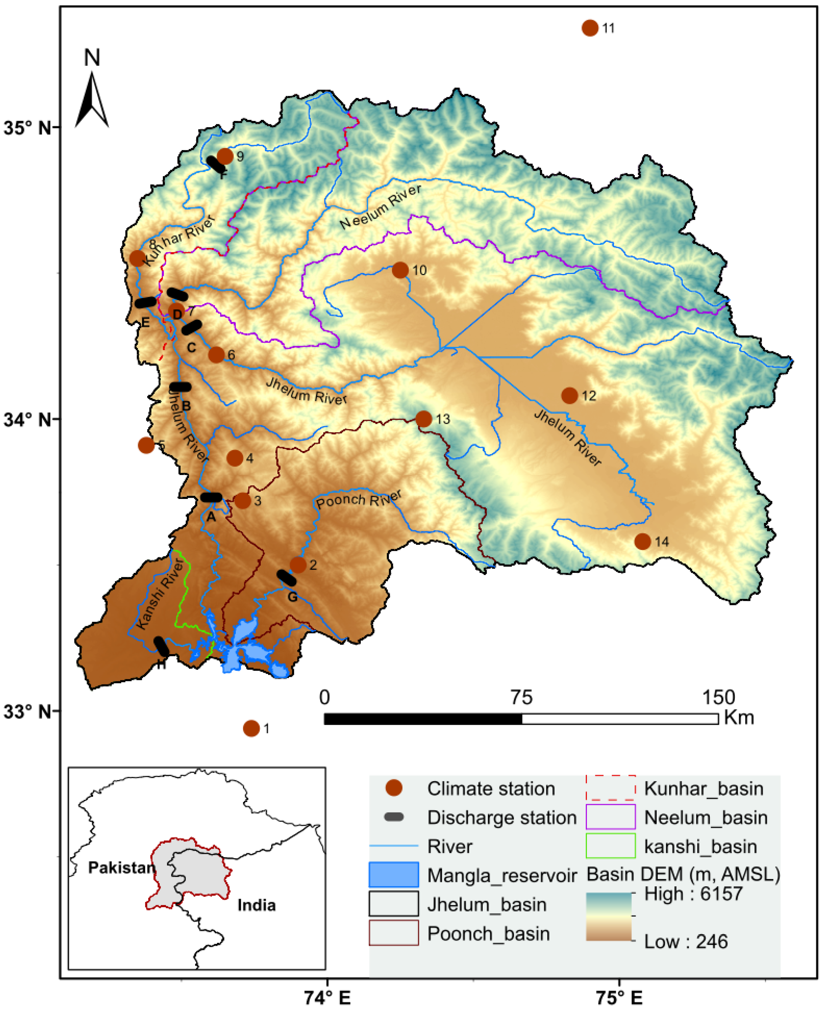
The Upper Jhelum River basin (UJRB) is situated in the north of Pakistan, a highly elevated area, as illustrated in Figure 1. This is one of the biggest streams of the Indus River basin. The Jhelum River, along with the Kunhar and Neelum Rivers, the major streams of the Jhelum River, drain the southern slope of the Greater Himalayas and the northern slope of the Pir Punjal Mountains are located in Jammu and Kashmir (Figure 1). The total area of the basin is about 33,342 km², and the elevation in the basin ranges between 200 m and 6248 m. The whole basin entirely drains into the Mangla Reservoir, the country’s second largest reservoir. The key purpose of the reservoir is to supply water for irrigation to 6 million hectares land of the country, and electricity is produced as a byproduct. The installed capacity of the reservoir is 1000 MW, which is 6% of the country’s installed capacity [1,24].

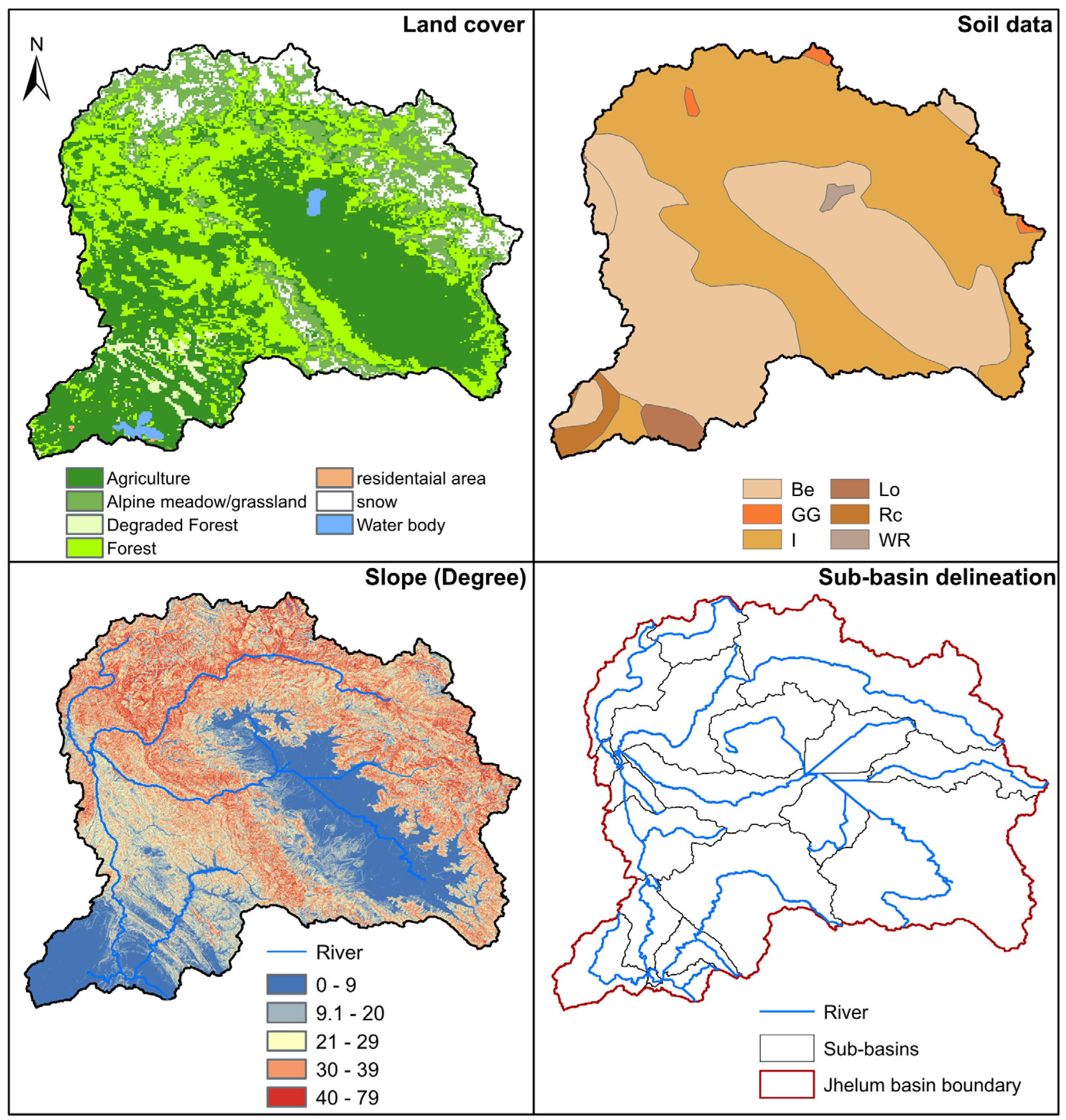
The basin has an undulating slope ranging from 0° to 79°, as shown in Figure 2. The plains along the course of the rivers, especially the lower parts (near the Mangla Reservoir) and the northeastern parts (near Srinagar valley) of the basin, are located on a gentle slope (0°–10°). However, most areas of the basin are located on a moderate (>10° and <30°) to steep slope (>30°).

A great diversity of vegetation such as temperate coniferous forest, subtropical coniferous forest, alpine meadow, grassland, and agricultural cover has been observed in the basin, as described in

Table 1. Basic characteristics of soil and land cover data in the Jhelum River basin.

Symbol	HWSD-Soil Group	Area		Texture	Top Soil Fraction		Clay (%)	TSGC
		%	km2		Sand (%)	Silt (%)		Gravel (%)
Be	Cambisols	46.3	15,441	Medium	40	35	25	9
GG	Gleysols	0.7	250	Medium	40	33	27	23
I	Lithosols	49.6	16,543	Medium	43	34	23	26
Lo	Luvisols	1.5	489	Course	81	9	10	4
Rc	Regosols	1.5	507	Medium	43	35	22	17
WR	Inland water	0.3	113	Medium	42	36	22	9
SR	Land use cover	Area		Land use cover
	Re-classes	%	km2	Original
1	Forest	28.9	732	Temperate Conifer/Subtropical Conifer/Tropical Moist Deciduous/Junipers
2	Degraded Forest	1.9	49	Degraded Forest
3	Alpine Meadow/grassland	15.6	396	Slope Grasslands/Sparse vegetation (cold)/Gobi/Desert (cold)/Alpine Meadow/Alpine Grassland
4	Agriculture	45.0	1140	Irrigated Agriculture/Slope Agriculture
5	Water body	0.8	19	Water body
6	Snow	7.8	197	Snow
7	Residential/Settlement	0.1	1	Residential/Settlement

and shown in Figure 2. However, the land covers were reclassified into seven main groups to explore the key land use covers in the basin. Agriculture, forest, and grassland are three major land-use covers covering areas of 45%, 29%, and 16% of the basin, respectively (Table 1).

Figure 2 and Table 1 also show the main soil groups in the Jhelum basin. Cambisols and Leptosols are two main soil groups, covering 46% and 50% of the basin, respectively. Cambisols are weak to moderate developed soils, and leptosols are very narrow soils over hard rock or unconsolidated gravelly material. Some glacier patches (less than 1% of the basin) are also available in the upper parts of the basin. Basic information about soil types is given in Table 1. The properties of soils were derived from the soil data of 1 km resolution in the basin.

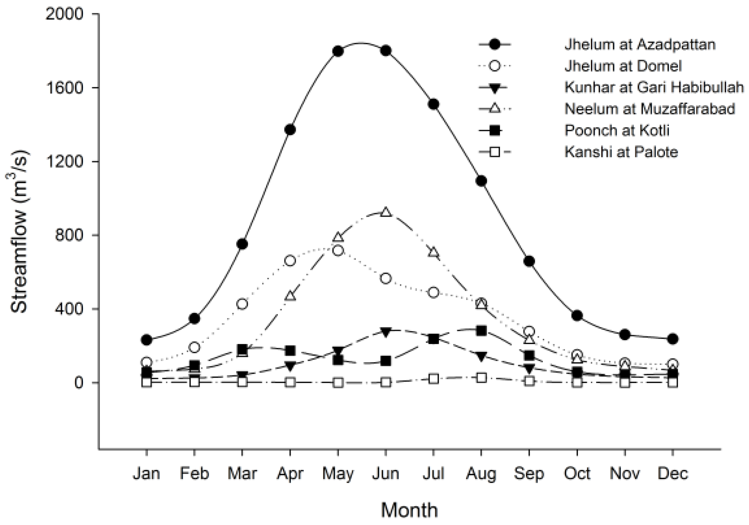
The Jhelum basin has a mean temperature and average annual precipitation of 13.72 °C and 1202 mm, respectively [1]. The mean streamflow at different hydrometric sites is described in

Table 2. Basic information about hydrometric stations in the Jhelum River basin.

ID	River	Station	Lat.	Long.	Elevation	Catchment Area	Period	Mean Discharge
			(°N)	(°E)	(m ASL)	(km2)	(Year)	(m3/s)	(mm/year)
A	Jhelum	Azad Pattan	33.73	73.60	455	26,088	1978–2000	829	1002
B	Jhelum	Kohala	34.11	73.50	584	24,549	1971–1995	779	1001
C	Jhelum	Domel	34.35	73.47	675	14,395	1976–2000	329	721
D	Neelum	Muzaffarabad	34.37	73.47	691	7415	1971–2000	356	1514
E	Kunhar	Garhi Habibullah	34.40	73.38	810	2335	1971–2000	105	1418
F	Kunhar	Naran	34.90	73.65	2421	1011	1971–2000	48	1497
I	Poonch	Kotli	33.46	73.88	516	3739	1971–2000	133	1122
J	Kanshi	Palote	33.22	73.43	400	1285	1971–2000	6	147

Notes: Lat.: latitude; Long.: longitude; m ASL: meters above sea level.

, calculated for the available periods. This shows that the mean annual discharge at Azad Pattan stream gauge is 829 m³/s (1002 mm), where about 80% area of the basin contributes. Monthly streamflows at different sites are presented in Figure 3. The streamflows at Muzaffarabad, Garhi Habibullah, Kotli, and Palote were calculated for the period 1971–2000, and at Azad Pattan and Domel for the periods 1978–2000 and 1976–2000, respectively. May to August are observed as high-flow months and October to February as low-flow months in the basin. In the basin, flows at different sites (Figure 3) start rising due to the melting of snowfall in March and April and reach the maximum states in May, June, and July due to the addition of monsoon rainfall (June–August). The maximum flows at Azad Pattan (1766 m³/s), Muzaffarabad (894 m³/s), and Garhi Habibullah (279 m³/s) occur in June, while the maximum flows occur in May at Domel (711 m³/s) and in August at Kotli (288 m³/s) and Palote (28 m³/s).

3. Data Description

3.1. Hydro-Climatic Data

The measured daily maximum temperature (Tmax), minimum temperature (Tmin), and precipitation (Prec) data for 14 meteorological stations were collected from Pakistan Meteorological Department (PMD), India Meteorological Department (IMD), and the Water and Power Development Authority (WAPDA) of Pakistan. For hydrological analysis, observed daily streamflow data of eight hydrometric stations were obtained from WAPDA. The geographic and basic information of hydro-meteorological stations are presented in Table 2 and

Table 3. Basic information about meteorological stations in the Jhelum River basin.

SN	Station	Latitude (°N)	Longitude (°E)	Elevation (m ASL)	Period (Years)
1	Jhelum	32.94	73.74	287	1970–2000
2	Kotli	33.50	73.90	614	1970–2000
3	Plandri	33.72	73.71	1402	1962–2000
4	Rawlakot	33.87	73.68	1676	1961–2000
5	Murree	33.91	73.38	2213	1970–2000
6	Garidopatta	34.22	73.62	814	1970–2000
7	Muzaffarabad	34.37	73.48	702	1961–2000
8	Balakot	34.55	73.35	995	1970–2000
9	Naran	34.90	73.65	2362	1961–2000
10	Kupwara	34.51	74.25	1609	1976–2000
11	Astore	35.34	74.90	2168	1953–2000
12	Srinagar	34.08	74.83	1587	1961–2000
13	Gulmarg	34.00	74.33	2705	1969–2000
14	Qazigund	33.58	75.08	1690	1961–2000

, and Figure 1.

3.2. Downscaled Climatic Data

Statistical Downscaling Model (SDSM) is a hybrid of multiple linear regression and a stochastic weather generator [25] and is broadly applied for downscaling of climate variables [1]. SDSM was used for downscaling of Tmax, Tmin, and Prec for the period 2011–2099 under A2 and B2 scenarios of HadCM3 in the Jhelum River basin. HadCM3 is a General Circulation Model (GCM) developed by the U.K. Meteorological Office. It has a spatial resolution of 2.5° × 3.75° (latitude × longitude), with a surface spatial resolution of about 278 × 417 km, decreasing to 278 × 295 km at 45 degrees North and South [26]. Scenario A2 defines a very heterogeneous world. It describes a very slow fertility pattern across regions, a continuous increase in global population, regionally oriented economic development, more fragmented and slower per capita economic growth, and more rapid technological changes relative to other scenarios. The B2 scenario describes the world with an emphasis on social and environmental sustainability as well as local solutions to economic. Under this scenario, the population of the world increases at a lower rate than under A2, and economic development is intermediate. B2 also gives an indication of less rapid and more diverse technological changes as compared to other scenarios, i.e., A1 and B1 [27].

A bias correction technique was also applied on the downscaled data to increase the accuracy in the results. After the calibration and validation of SDSM, it was observed that the statistical indicators, the coefficient of determination and RMSE, were not satisfactory, especially in cases of precipitation. So, after the application of BC, much improvement was observed in the statistical indicators, especially in cases of precipitation. The results have shown that Tmax, Tmin, and Prec are projected to increase by 0.91–3.15 °C, 0.93–2.63 °C, and 6%–12% under A2, respectively, and 0.69–1.92 °C, 0.56–1.63 °C, and 8%–14% under B2, respectively [1].

3.3. Digital Elevation Data

Elevation data are an important source of the ancillary data used in hydrological studies. A digital elevation model (DEM) is a representation of elevation data in a digital format that is globally used to extract topographical characteristics of a terrain [28,29]. In the present study, a DEM of 30 m, created by the Advanced Spaceborne Thermal Emission and Reflection Radiometer (ASTER), was obtained from the U.S. Geological Survey (USGS) (http://gdex.cr.usgs.gov/gdex/), as presented in Figure 1.

In the present study, HEC-GeoHMS, an extension of GIS, was used to extract the basin parameters from DEM such as slopes of rivers and sub-basins, areas of sub-basins, river length, longest flow paths of sub-basins, elevation in the basin, flow direction, streamlines, contour lines, and aspects during the process of watershed delineation. However, only the slope and delineated sub-basins are shown in Figure 2. Twenty sub-basins were delineated for hydrological process.

3.4. Land Use and Soil Data

Land cover can significantly affect the hydrologic processes in a region. These processes are mostly affected by the morphology of plant species and the density of plant cover [30]. The land cover data for the Jhelum River basin were extracted from the global land cover data of 1 km resolution established by the Joint Research Center (JRC) of European Commission (http://eusoils.jrc.ec.europa.eu/data.html), as shown in Figure 2.

The soil data for the basin were obtained from the Harmonized World Soil Database, with a resolution of 1 km, as shown in Figure 2. This database was developed by the Food and Agriculture Organization (FAO) with the collaboration of International Institute Of Applied Systems Analysis (IIASA), the International Soil Reference and Information Centre (ISRIC), the Institute of Soil Science of Chinese Academy of Sciences (ISSCAS), and the Joint Research Centre (JRC) of the European Commission (http://www.fao.org/soils-portal/soil-survey/soil-maps-and-databases/harmonized-world-soil-database-v12/en/).

The soil and land cover data were used to extract the initial estimations about the hydrological properties of the basin such as maximum moisture deficit, hydraulic conductivity, crop coefficient, percentage of imperviousness, and basin lag. However, the exact estimations of these parameters for each sub-basin were obtained only during the calibration process.

4. Methodology

4.1. HEC-HMS’s Description

The Hydrologic Engineering Center-Hydrological Modeling system (HEC-HMS) is a rainfall–runoff simulation model. The model has been used for a wide range of basins from small urban areas to large river watersheds. The model was formulated by the U.S. Army Corps of Engineers at the Hydrologic Engineering Center. HEC-HMS comprises six loss methods (e.g., initial and constant method and SCS curve number method) to estimate excess precipitation, seven translation techniques (e.g., Clark and SCS unit hydrograph methods) to calculate the direct runoff from excess precipitation, five base flow estimation methods (e.g., constant monthly and recession methods), and six channel routing methods (e.g., Muskingum and modified pulse methods). In HEC-HMS, meteorological model is used to gather information about meteoroidal data (precipitation, temperature, and evapotranspiration, etc.) and to prepare meteorological boundary conditions for each sub-basin. The meteorological model consists of different kind of methods for precipitation interpolation, evapotranspiration estimation, and snowmelt calculation. There are four major components for a complete setup of HEC-HMS in a basin: (1) a basin model; (2) a meteorological model; (3) a control specification; and (4) input time series. These must be properly linked with each other for accurate operation. The basin model shows the physical features of a watershed such as stream length, sub-basin area, slope of basin, and laps rate. It comprises four methods: (1) a loss method; (2) a base flow method; (3) a transforming method; and (4) a channel routing method. Control specification is used to control the simulation period. For example, it controls when the model is to start and stop, and what the simulated time interval should be. The input time series consists of all climatic data required for the model such as temperature, precipitation, streamflow, wind speed, and evapotranspiration. These time series are directly linked with the meteorological model to calculate excess precipitation and to the basin model to simulate streamflow. A complete description of the model formulation and its various processes is available in the User’s Manual and Technical Reference Manual of HEC-HMS [31,32].

In this study, the deficit and constant loss (DCL) method, the SCS unit hydrograph method, Muskingum method, and the recession method were included in the basin-model setup for excess-precipitation calculation, direct-runoff transformation, channel routing, and base-flow estimation, respectively. Gauge weights, temperature index, and monthly evapotranspiration methods were included for the setup of meteorological model. The same combination has been used in some previous studies like Meenu et al. [18], Verma et al. [19], and Shrestha et al. [33].

DCL is a single layer continuous method for the estimation of soil moisture changes. The method contains four main estimation parameters: (1) initial deficit; (2) constant rate; (3) maximum deficit; and (4) impervious percentage. These parameters are firstly estimated using soil and land cover data as initial inputs to the model but are finalized only during the calibration process.

After the calculation of excess precipitation by DCL, the SCS unit hydrograph method transforms this precipitation into direct surface runoff. In SCS, basin lag is the only parameter that is needed to estimate during the calibration. An initial value for basin lag can also be estimated by multiplying a factor of 0.6 by the time of concentration of a basin. The recession method, which calculates the base flow of a basin, needs three parameters (i.e., recession constant, initial discharge, and threshold) to be optimized. The Muskingum method, which is used to transfer the total flow (surface and base flow) through the channels, is a simple mass conservation scheme; it requires two parameters, Muskingum coefficient (X) and travel time (K), to be finalized during the calibration. The X value varies between 0 and 0.5.

For the setup of a meteorological model, a Thiessen polygon was applied to allocate the weights to each site (climatic gauge) in the basin. This method is useful when gauges are scarce in a basin as compared to the basin area, as in [18,33]. For snowmelt modeling, each sub-basin was divided into different elevation bands (ranging from 3 to 5) for proper application of the temperature index method (TIM). TIM is an extension of the degree-day technique to calculate flow from snowpack. In the degree-day approach, a fixed amount of snowmelt is assigned for each degree above freezing point. This method is a conceptual representation of the cold energy stored in the snowpack. This also takes care of past conditions and some other climatic factors during the calculation of snowmelt. Different parameters such as base temperature, wet melt rate, rain rate limit, melt rate pattern, lapse rate, and antecedent temperature index are required for this method [31]. An average lapse rate of −7.0° per km in the basin was calculated by plotting the average temperatures of climatic stations against the altitudes at which they are located. A standard method for the calculation of potential evapotranspiration, the Penman–Monteith method [20], was applied in this study. A schematic diagram for the setup of HEC-HMS in the Jhelum River basin is shown in Figure 4. This shows the rainfall and flow calculation points for each sub-basin and flow direction lines in the basin.

4.2. Calibration and Validation of HEC-HMS

In this study, a split sample technique was chosen for the calibration and validation of HEC-HMS. In this technique, the calibration period does not overlap with the validation period. According to data availability and consideration of missing values, the period 1982–1989 was chosen for the calibration of the model and the period 1978–1981 for the validation. The land-use cover and soil characteristics of the Jhelum basin were considered to be constant during the simulation periods.

For the evaluation of model’s performance, three popular indicators, namely, the coefficient of determination (R²), percent deviation (D), and Nash–Sutcliffe efficiency (E), were calculated from the measured and simulated flows. The R² values indicate how well the simulated flow follows the variations of the measured flow, D describes the mean percent deviation between the simulated and measured flows, and E illustrates how well the simulated plot fits with the observed one [18]. For better illustration, the measured flow was also compared graphically with the simulated flow to analyze the variations in the low and high flows. In this study, the calibration and validation of the model was done at different hydrometric sites available in the basin.

The performance indicators (R², D, and E) were calculated by the following equations:

$$R^2=\frac{\sum \left(Q_{obs}-\overline{Q_{obs}}\right)\times \left(Q_{sim}-\overline{Q_{sim}}\right)}{\sqrt{\sum {\left(Q_{obs}-\overline{Q_{obs}}\right)}^2\times {\left(Q_{sim}-\overline{Q_{sim}}\right)}^2}}$$

(1)

where $Q_{obs}$ and $Q_{sim}$ are observed and simulated values, respectively. The value of R² should be closer to 1 for a good correlation between the simulated and observed flows. The correlation is considered optimal if R² is exactly equal to 1 [18].

$$D(\%)=100\times \frac{\sum \left(Q_{sim}-Q_{obs}\right)}{\sum Q_{obs}}$$

(2)

A D value of 0% indicates a perfect model. The positive and negative values of D are indications of overestimation and underestimation, respectively [18].

$$E=1-\frac{\sum {\left(Q_{sim}-Q_{obs}\right)}^2}{\sum {\left(Q_{obs}-\overline{Q_{obs}}\right)}^2}$$

(3)

E ranges from 0 to 1. Positive values closer to 1 are indications of good results. However, negative values closer to 0 are not acceptable. The results are considered to be good if the values of E are greater than 0.75 and satisfactory if E values lie between 0.36 and 0.75 [34].

4.3. Future Changes in Streamflow

After successful calibration and validation, the downscaled temperature and precipitation time series for the period 1971 to 2099 (A2 and B2) were fed into HEC-HMS to simulate daily flow (surface flow and base flow) at different sites in the Jhelum basin. Although physical characteristics change with time, these were kept constant throughout the simulation period. The simulated flow was split into three future periods—2020s (2011–2040), 2050s (2041–2070), and 2080s (2071–2099)—and one baseline period (1971–2000). The flows of the future periods were compared with the baseline flow to assess the future changes in the basin, as done by [29,35]. The absolute observed seasonal and annual values were also calculated for the period 1971–2000. These values can be used to observe the absolute streamflow values in the future. Since the flow data at Azad Pattan and Domel sites start from 1978 to 1976 respectively, (Table 2), the streamflow was simulated at these sites for the period 1971–1977 using the observed meteorological data feeding into HEC-HMS, after calibration and validation of the model. Similarly, at Kohala, flow data were generated for the period 1996–2000 because data are not available for this period at this site. The following indicators were used to assess the future changes with respect to the simulated baseline flow under A2 and B2 scenarios: mean flow, low flow, median flow, high flow, and temporal shifts in center-of-volume dates. To find the timing of streamflow under climate change conditions, an indicator center-of-volume date (CVD)—a date at which half of the total volume of annual flow passes though at a specific site and in a specific time period—was used in this study and calculated by the equation given in Stewart et al. [36].

5. Results and Discussion

5.1. Calibration and Validation of HEC-HMS

Table 4. Nash–Sutcliffe efficiency (E), coefficient of determination (R²), and percent deviation (D) for calibration (1982–1989) and validation (1978–1981) for different stream gauges in the Jhelum River basin.

Station	River	Calibration			Validation
		E	R2	D (%)	E	R2	D (%)
Naran	Kunhar	0.74	0.75	−11.00	0.71	0.78	7.62
Garhi Habibullah	Kunhar	0.65	0.67	−9.92	0.71	0.74	2.53
Muzaffarabad	Neelum	0.72	0.73	−11.73	0.75	0.81	12.4
Domel	Jhelum	0.66	0.66	−2.38	0.62	0.63	−3.04
Kohala	Jhelum	0.72	0.73	−8.54	0.78	0.8	6.34
Azad Pattan	Jhelum	0.70	0.71	−8.44	0.75	0.78	8.71
Kotli	Poonch	0.31	0.36	1.21	0.32	0.35	0.14

shows the model performance parameters (E, D, and R²) for the calibration (1982–1989) and validation (1978–1981) periods at different gauging stations in the basin. The E and R² values were ranged from 0.31 to 0.75 for the calibration period and 0.32 to 0.81 for the validation period, and the D values stretched from −12.00% to 1.00% for calibration and −3.00% to 12.00% for validation. It was observed that the model overestimated during the validation period but underestimated during the calibration period. This might be due to keeping the land use characteristics constant throughout the simulation periods (calibration and validation periods). The E and R² values were greater than 0.60 at all gauging stations except on Kotli, which is an indication of satisfactory results. These results can be improved if the temperature and precipitation data are interpolated along the altitude in the basin, which can increase the efficiency of the temperature index model, used for snowmelt calculation, as well as the rainfall–runoff model.

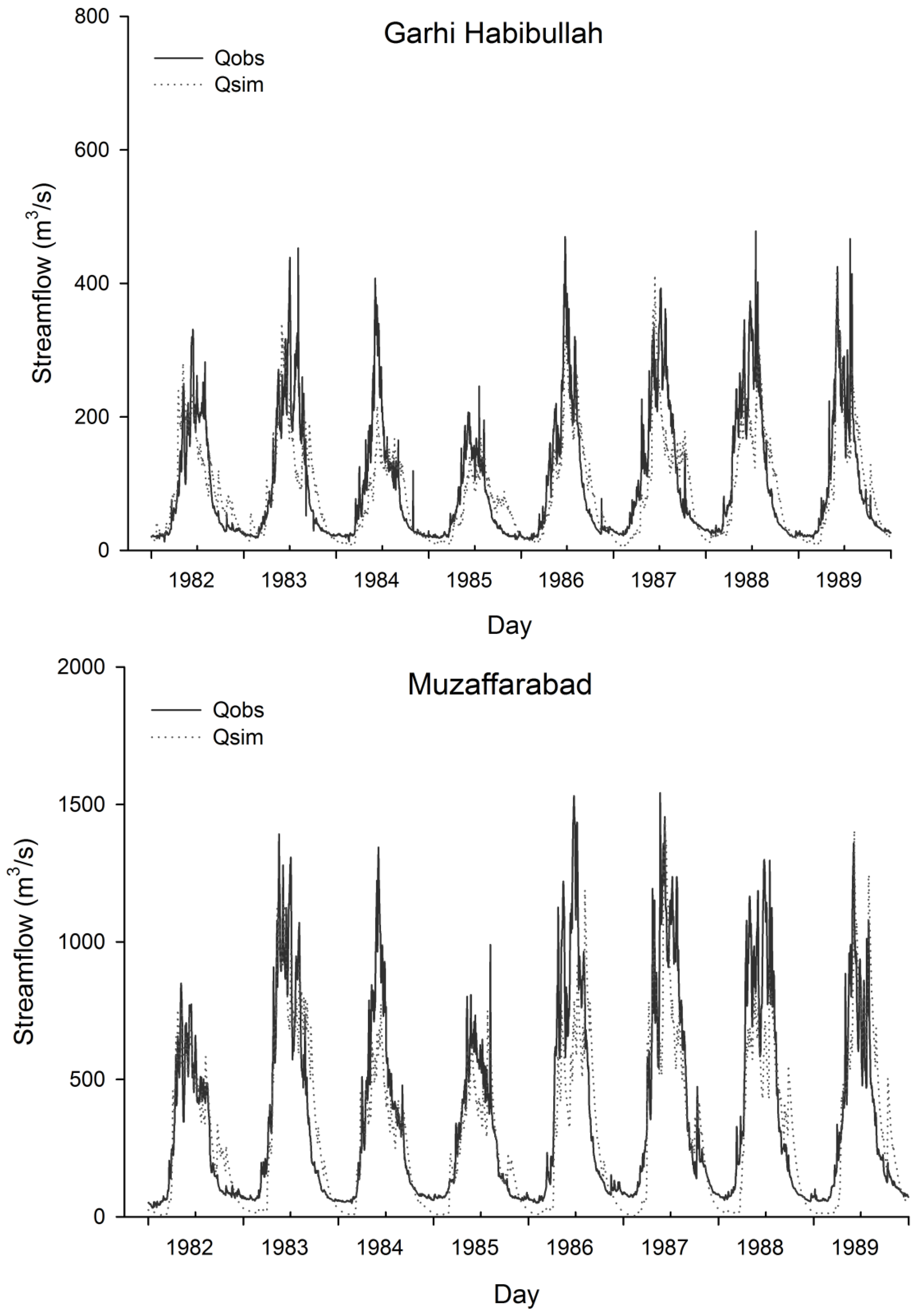
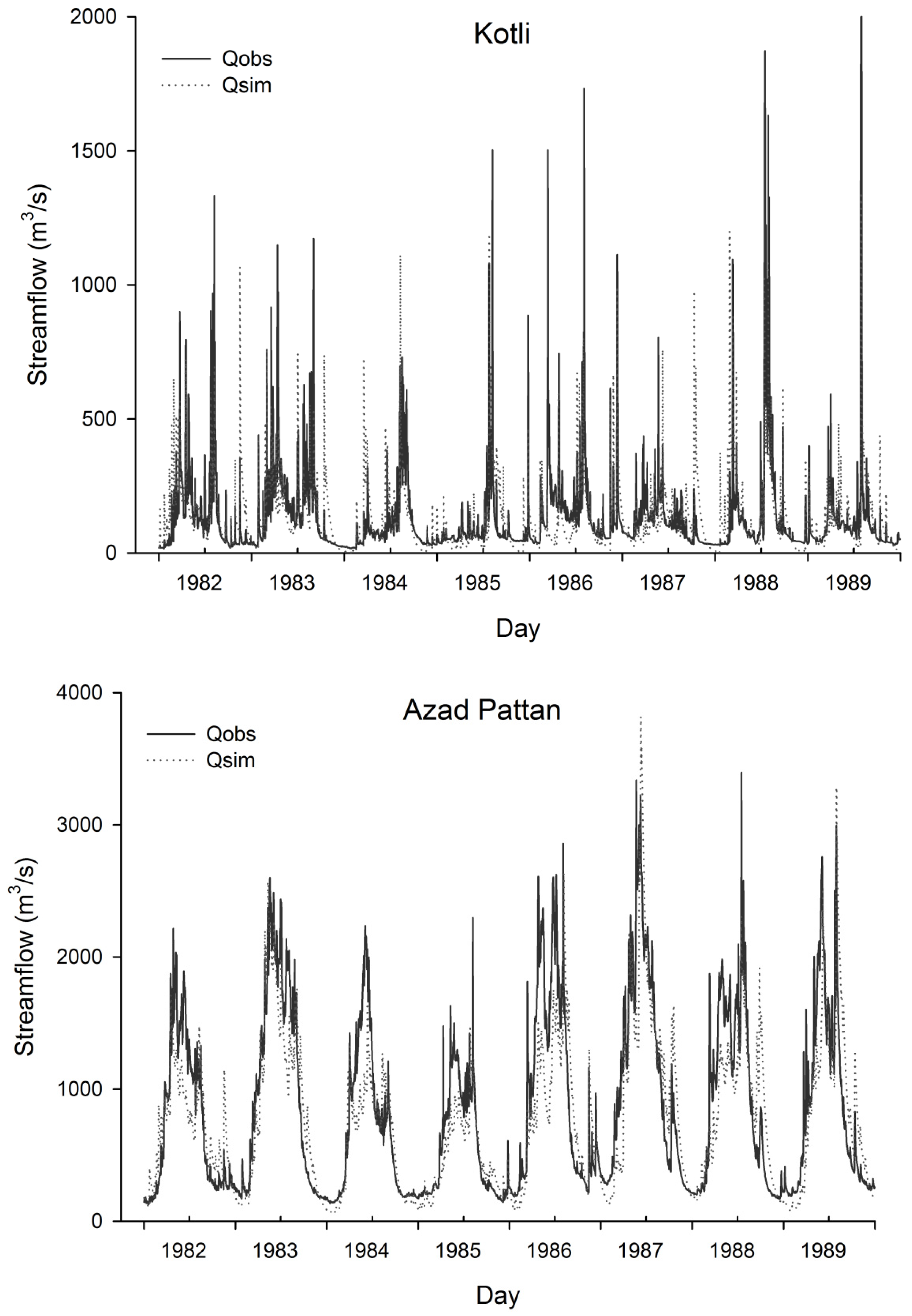
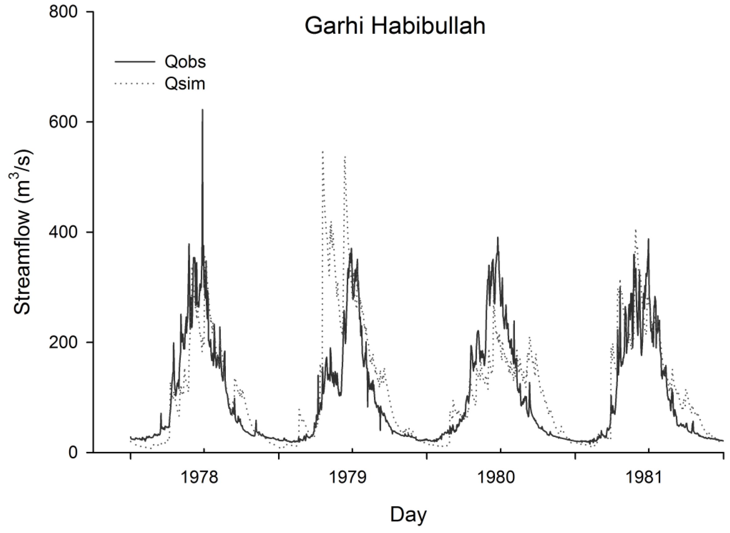
Figure 5 and Figure 6 show graphical comparisons of the measured flows against the modeled flows at different gauges for the calibration and validation periods, respectively. At all gauging stations except Kotli, the patterns of measured flows were well captured by the patterns of modeled flows during the calibration and validation periods. However, the peak and low flows were not well estimated by the model at some stations like Garhi Habibullah, Domel, and Kotli. Bad results at Kotli may be due to high fluctuation in daily flow, few rain gauges, and a steep slope.

5.2. Future Changes in Mean Streamflow

Table 5. Future changes (%) in streamflow at different gauges relative to the baseline (1971–2000) under the A2 and B2 scenarios in the Jhelum River basin.

	Naran	Garhi Habibullah	Muzaffarabad	Domel	Kohala	Azad-Pattan
Observed/Simulated A2/Simulated B2 mean streamflow (m3/s) for the baseline period
Winter	10/3/3	25/21/22	74/57/59	125/98/97	241/196/197	263/208/206
Spring	37/26/29	110/78/88	504/461/487	586/350/335	1213/930/946	1259/970/987
Summer	121/180/176	226/321/305	682/857/835	521/592/552	1395/1857/1764	1446/1941/1841
Autumn	24/47/49	58/121/112	165/315/298	218/353/316	396/832/766	418/858/794
Annual	48/64/64	105/135/132	356/422/420	362/348/325	811/954/918	847/994/957
Changes (%) in 2020s A2 (B2)
Winter	12.0 (−2.9)	20.0 (12.2)	10.4 (5.9) 5.5 (8.6)		23.5 (22.1)	31.1 (31.3)
Spring	12.2 (8.9)	30.1 (21.5)	10.6 (2.6)	12.0 (21.4)	14.0 (14.6)	12.6 (14.7)
Summer	0.2 (6.2)	−7.2 (−1.6)	−8.1 (−3.6)	−10.1 (−2.4)	−9.8 (−3.6)	−11.1 (−4.4)
Autumn	8.7 (−5.2)	3.3 (1.5)	0.1 (−1.4)	−8.7 (1.3)	−1 (2.6)	1.9 (5.5)
Annual	8.3 (1.7)	11.6 (8.4)	3.3 (0.9)	−0.3 (7.2)	6.7 (8.9)	8.6 (11.7)
Changes (%) in 2050s A2 (B2)
Winter	9.1 (−2.1)	14.8 (2)	8.9 (−5.6)	5.7 (4.1)	7.9 (0.8)	5.7 (2.4)
Spring	30.8 (28.7)	10.6 (2)	7.6 (4.4)	1.8 (10.5)	5.4 (6.5)	4.0 (5.4)
Summer	−1.0 (5.0)	−2.9 (1.9)	−1.1 (1.6)	3.4 (11.8)	−0.2 (5.0)	−0.2 (5.1)
Autumn	5.1 (−3.0)	1.8 (−1.9)	−0.7 (−5.3)	−4.3 (8.9)	−2.6 (2.2)	−2.4 (3.3)
Annual	11.0 (7.2)	6.1 (1.0)	3.7 (−1.2)	1.6 (8.8)	2.6 (3.6)	1.8 (4.0)
Changes (%) in 2080s A2 (B2)
Winter	13.4 (5.4)	31 (15.8)	17.4 (11.5)	20.8 (18.5)	29.7 (28.2)	37.8 (39.1)
Spring	49.3 (38.4)	31.8 (27.3)	11.0 (5.0)	11.6 (9.3)	11.5 (9.4)	9.6 (7.6)
Summer	6.1 (3.7)	−0.2 (3.3)	−10.1 (−6.1)	−13.3 (−5.7)	−10.4 (−4.8)	−11.8 (−5.7)
Autumn	12.2 (−0.1)	11.1 (18.4)	1.2 (6.8)	−4.8 (15.7)	1.4 (14.0)	5.0 (17)
Annual	20.2 (11.8)	18.4 (16.2)	4.9 (4.3)	3.6 (9.4)	8.0 (11.7)	10.1 (14.5)

describes the projected flow changes (in percentage) in the 2020s, 2050s, and 2080s with respect to the simulated flow for the baseline period (1971–2000) under A2 and B2 scenarios. The absolute seasonal and annual values of the observed flow and simulated flows (A2 and B2) for the baseline period are also described in Table 5. The mean annual flows in the Kunhar River at Garhi Habibullah, Neelum River at Muzaffarabad, and Jhelum River at Domel are 105 m³/s, 356 m³/s, and 362 m³/s, respectively, for the baseline period. The mean annual flow of the Jhelum River at Azad Pattan (after merging of the Kunhar and Neelum Rivers into the Jhelum River) is 847 m³/s for the baseline.

In all three periods and under both scenarios, the mean flows in winter (DJF), spring (MAM), and autumn (SON) seasons were projected to increase at most of the gauges in the basin. Conversely, in summer (JJA), which is the peak flow season, the flows were projected to decrease at most of the sites in the future under both scenarios, especially under A2. In the 2020s, a maximum increase of 30%, 11%, and 12% was calculated in spring, respectively, at Garhi Habibullah on the Kunhar River, Muzaffarabad on the Neelum River, and Domel on the Jhelum Rive under A2. On the other hand, maximum increases of 24% and 31% at Kohala and Azad Pattan, respectively, were projected in winter under A2. Conversely, summer showed a maximum decrease of 11% at Azad Pattan, 8% at Muzaffarabad and 7% at Garhi Habibullah. In the 2050s, although the patterns of projected changes were similar to the changes in the 2020s, the magnitudes of these changes were lower than in the 2020s. In the 2080s, the pattern of seasonal and annual changes was the same as in previous periods, but the magnitudes were higher, especially than the 2050s. Winter showed a maximum projected increase in the basin (at Azad Pattan) under both scenarios at the end of this century. On the whole, the mean annual flow was projected to increase by about 9 (12)%, 2 (4)%, and 10 (15)% in the 2020s, 2050s, and 2080s, respectively, under A2 (B2) at Azad Pattan in the basin. It was observed that streamflow was projected to decrease during the 2050s relative to the 2020s and then increased again in the 2080s. The results for Kotli gauging station were not included in the present study because, during calibration and validation, the results were not satisfactory.

5.3. Future Changes in Low, Median, and High Flows

The projected changes in high, median, and low flows at different gauging stations are outlined in

Table 6. Future changes (%) in low, median, and high flows with respect to the baseline (1971–2000) under A2 and B2 scenarios in the Jhelum River basin.

	Naran	Garhi Habibullah	Muzaffarabad	Domel	Kohala	Azad Pattan
Observed/Simulated A2/Simulated B2 high, low, and median flows (m3/s) for the baseline period
Q5	170/235/230	316/399/393	1078/1102/1107	848/787/720	2142/2218/2178	2205/2315/2256
Q50	19/24/27	54/79/80	194/333/324	306/314/298	606/826/789	687/848/814
Q95	8/1/1	21/14/15	53/34/34	64/60/60	151/127/131	166/137/139
Changes in 2020s A2 (B2)
Q5	1.6 (5.1)	−7.5 (−4.2)	−6.5 (−1.6)	−9.9 (7.6)	−8.3 (−2.5)	−9.9 (−3.4)
Q50	12.3 (−7.2)	14.7 (11.4)	0.2 (−4.7)	−1.0 (7.1)	3.1 (1.3)	5.5 (4.3)
Q95	0.0 (0.0)	11.3 (11.0)	4.2 (−0.3)	6.8 (3.9)	26.2 (22.7)	28.8 (28.5)
Changes in 2050s A2 (B2)
Q5	0.1 (7.8)	−3.1 (−2.5)	−0.9 (1.6)	4.2 (17.1)	0.6 (4.3)	0.1 (4.3)
Q50	12.8 (1.3)	6.2 (1.5)	−3.8 (−4.7)	−0.4 (5.4)	−3.0 (2.0)	−2.3 (3.2)
Q95	0.0 (0.0)	15.6 (9.0)	5.4 (−5.3)	8.0 (4.9)	8.4 (1.2)	6.4 (2.5)
Changes in 2080s A2 (B2)
Q5	9.4 (5.3)	1.2 (−0.4)	−6.7 (−9.2)	−16.8 (−3.1)	−8.7 (−8.4)	−10.5 (−9.4)
Q50	26.1 (2.8)	20.6 (25.5)	−3.4 (3.4)	3.3 (11.0)	2.0 (12.9)	5.2 (15.4)
Q95	0.0 (0.0)	21.3 (14.5)	6.9 (4.1)	11.0 (12.8)	21.1 (19.5)	23.7 (26.4)

Notes: Q₅: high flow; Q₅₀: median flow; Q₉₅: low flow.

for three future periods relative to the baseline period under A2 and B2 scenarios. Absolute values of high, median, and low flows calculated from the observed flow and simulated flow, under A2 and B2, for the baseline period are also described in Table 6. The high, median, and low flows in the basin are 2205 m³/s, 687 m³/s, and 166 m³/s at the Azad Pattan, respectively. In the basin, the high flows were projected to decrease at most of the sites; conversely, low and median flows were projected to increase at most of the sites. In the Kunhar River (at Garhi Habibullah), high, low, and median flows were simulated to increase under both scenarios at the end of this century except the high flow under B2. On the other hand, in the Neelum River basin (at Muzaffarabad), high flow was projected to decrease under both scenarios at the end of the 21st century, but low flow was projected to increase. The low and median flows in the Jhelum River at Dome showed an increase, but a decrease in high flow was calculated under both scenarios at the end of the 21st century. At Azad Pattan, the major site in the basin, about 5%–15% and 24%–26% increases in median and low flows, respectively, were projected under both scenarios in the 2080s but a 9%–10% decrease in high flow.

5.4. Projected Shifts in Center-of-Volume Date (CVD)

The projected CVD changes in the 2020s, 2050s, and 2080s relative to the baseline period at different sites under A2 and B2 scenarios are outlined in

Table 7. Future changes in center-of-volume dates (CVDs) with respect to the baseline (1971–2000) at different stream flow stations under both scenarios, A2 and B2, in the Jhelum River basin.

River	Station	CVDs for the Baseline Period		2020s	2050s	2080s
		Day of Year (Observed/Simulated A2/Simulated B2)		Changes (Day) under A2 (B2)
Kunhar	G. Habib	183/201/199	2 July/20 July/18 July	−3 (−2)	−1 (0)	−9 (−1)
Neelum	M. Abad	173/188/186	22 June/7 July/5 July	−2 (−1)	−1 (−2)	−7 (−1)
Jhelum	Domel	169/196/194	18 June/15 July/13 July	−5 (−4)	0 (−1)	−9 (−2)
Jhelum	Azad Pattan	169/193/191	18 June/12 July/10 July	−3 (−2)	−1 (−1)	−7 (−2)

. The absolute CVD values calculated from the observed and simulated flows (A2 and B2) for the period 1971–2000 are also described in the table. The positive and negative values show a shift ahead in CVD and a shift back in CVD, respectively. For example, if a change in CVD value is 10 days with respect to the present CVD value (e.g., CVD = 2 July), this means that the CVD value will be shifted 10 days ahead in July and will be 12 July. The CVD values were 2 July in the Kunhar basin (at Garhi Habibullah site), 22 June in the Neelum basin (Muzaffarabad), 17 June in the Jhelum basin (Domel and Azad Pattan), and 22 June in the Poonch basin (Kotli), calculated from the observed data for the period 1971–2000. These CVD values in the 2020s, 2050s, and 2070s were projected to shift back by 1–5 days, 0–2 days, 1–9 days, respectively, at different sites in the basin under both scenarios, with respect to the baseline. This means that about half of the annual flow would pass by the Azad Pattan site one week earlier than at present.

6. Conclusions

The economy of Pakistan is highly based on agriculture and water is the primary factor for agriculture. However, Pakistan is included in the list of the most water-stressed countries in the world, and its water resources are greatly vulnerable to changing conditions of climate. This study assesses the impacts of a changing climate on the water resources of the transboundary Jhelum River basin in India and Pakistan, under A2 and B2 scenarios of HadCM3. The Jhelum River is a major stream of the Indus River, and is the sole source of the Mangla Reservoir, the second largest dam in Pakistan, which is used for irrigation and power production.

A hydrologic model, HEC-HMS, was calibrated and validate for the periods 1982–1989 and 1978–1981, respectively, at different hydrometric stations. Three indicators, i.e., the coefficient of determination (R²), Nash Efficiency (E), and percent deviation (D), and graphical presentations between the observed and modeled flows were used for the evaluation of the model’s performance. Downscaled temperature and precipitation data under A2 and B2 scenarios of HadCM3 were obtained from Mahmood and Babel [1] for the period 1971–2099, and these data were fed into HEC-HMS to simulate streamflow. The simulated flow data was divided into three future periods (2011–2040, 2041–2070, and 2071–2099) and one baseline period. The future periods were compared with the simulated flow of the baseline period (1971–2000) to assess the future changes. Different indicators, i.e., mean flow, low flow, median flow, high flow, and center-of-volume dates, were used to examine the changes in streamflow under A2 and B2 scenarios for these future periods.

Mean annual flow was projected to increase in the basin under both A2 and B2 scenarios, with a 4%–15% increase in future. The flows in winter, spring, and autumn were projected to increase at most of the sites but decrease in summer (the monsoon season). The projected increase in annual flow was maximum in the 2080s and minimum in the 2050s. This means the annual flow in the future will increase in the 2020s, reduce in the 2050s relative to the 2020s, and then increase again in the 2080s. An overall increase in low and median flows was predicted in the basin (at Azad Pattan gauge, with more than 80% of the flow) at the end of this century under A2 and B2. However, high flows were projected to decrease in future under both scenarios. Half of the volume of annual flow was projected to shift back about one week in the future.

On the whole, the Jhelum basin is likely to face increased flow on an annual and seasonal basis in the future, except in the summer. The basin would also face more temporal and magnitudinal variations in mean flow and peak flow in the future. This could create many complications for policymakers and managers of water resources if they do not consider changing climate conditions in the basin. For further studies on the basin, the main recommendation is to use the outputs of more than one GCM, so the uncertainties exhibited to GCMs can be investigated, and the potential impacts of climate change can be explored on the water resources in the basin.

7. Limitations of the Study

In the present study, the water resources of the Jhelum River basin were assessed under changing climate conditions by using only a single GCM (HadCM3), although it is suggested to use more than one GCM to explore the uncertainties related to the GCM’s outputs. Meteorological stations are scarce in the basin, which can cause low performance during the calibration and validation processes of a hydrologic model. The land cover and soil properties were kept constant throughout the simulation periods, which can affect the projections of streamflow in the basin.

References

1. Mahmood, R.; Babel, M.S. Evaluation of SDSM developed by annual and monthly sub-models for downscaling temperature and precipitation in the Jhelum basin, Pakistan and India. Theor. Appl. Climatol. 2013, 113, 27–44. [Google Scholar] [CrossRef]
2. Chu, J.; Xia, J.; Xu, C.Y.; Singh, V. Statistical downscaling of daily mean temperature, pan evaporation and precipitation for climate change scenarios in Haihe River, China. Theor. Appl. Climatol. 2010, 99, 149–161. [Google Scholar] [CrossRef]
3. IPCC. Climate Change 2013: The Physical Science Basis; Contribution of Working Group I to the Fifth Assessment Report of the Intergovern-Mental Panel on Climate Change; Cambridge University Press: Cambridge, UK; New York, NY, USA, 2013; p. 1535. [Google Scholar]
4. IPCC. Climate Change 2007: The Physical Science Basis; Solomon, S., Qin, D., Manning, M., Chen, Z., Marquis, M., Averyt, K.B., Tignor, M., Miller, H.L., Eds.; Contribution of Working Group I to the Fourth Assessment Report of the Intergovernmental Panel on Climate Change; Cambridge University Press: Cambridge, UK, 2007. [Google Scholar]
5. Khattak, M.S.; Babel, M.S.; Sharif, M. Hydro-meteorological trends in the Upper Indus River basin in Pakistan. Clim. Res. 2011, 46, 103–119. [Google Scholar] [CrossRef]
6. Zhang, X.C.; Liu, W.Z.; Li, Z.; Chen, J. Trend and uncertainty analysis of simulated climate change impacts with multiple GCMS and emission scenarios. Agric. For. Meteorol. 2011, 151, 1297–1304. [Google Scholar] [CrossRef]
7. Wang, H.; Zhang, M.; Zhu, H.; Dang, X.; Yang, Z.; Yin, L. Hydro-climatic trends in the last 50 years in the lower reach of the Shiyang River basin, NW China. CATENA 2012, 95, 33–41. [Google Scholar] [CrossRef]
8. Akhtar, M.; Ahmad, N.; Booij, M.J. The impact of climate change on the water resources of Hindukush-Karakorum-Himalaya region under different glacier coverage scenarios. J. Hydrol. 2008, 355, 148–163. [Google Scholar] [CrossRef]
9. Jetly, R. Pakistan in Regional and Global Politics; Taylor & Francis: New Delhi, India, 2012. [Google Scholar]
10. Gebremeskel, S.; Liu, Y.B.; de Smedt, F.; Hoffmann, L.; Pfister, L. Analysing the effect of climate changes on streamflow using statistically downscaled GCM scenarios. Int. J. River Basin Manag. 2005, 2, 271–280. [Google Scholar] [CrossRef]
11. Ahmadalipour, A.; Rana, A.; Moradkhani, H.; Sharma, A. Multi-criteria evaluation of CMIP5 GCMS for climate change impact analysis. Theor. Appl. Climatol. 2015, 1–17. [Google Scholar] [CrossRef]
12. Wilby, R.L.; Hay, L.E.; Gutowski, W.J.; Arritt, R.W.; Takle, E.S.; Pan, Z.; Leavesley, G.H.; Martyn, P.C. Hydrological responses to dynamically and statistically downscaled climate model output. Geophys. Res. Lett. 2000, 27, 1199–1202. [Google Scholar] [CrossRef]
13. Gädeke, A.; Hölzel, H.; Koch, H.; Pohle, I.; Grünewald, U. Analysis of uncertainties in the hydrological response of a model-based climate change impact assessment in a subcatchment of the Spree River, Germany. Hydrol. Process. 2014, 28, 3978–3998. [Google Scholar] [CrossRef]
14. Fowler, H.J.; Wilby, R.L. Beyond the downscaling comparison study. Int. J. Climatol. 2007, 27, 1543–1545. [Google Scholar] [CrossRef]
15. Ahmad, Z.; Hafeez, M.; Ahmad, I. Hydrology of mountainous areas in the Upper Indus basin, northern Pakistan with the perspective of climate change. Environ. Monit. Assess. 2012, 184, 5255–5274. [Google Scholar] [CrossRef] [PubMed]
16. Shrestha, M.; Koike, T.; Hirabayashi, Y.; Xue, Y.; Wang, L.; Rasul, G.; Ahmad, B. Integrated simulation of snow and glacier melt in water and energy balance-based, distributed hydrological modeling framework at Hunza River basin of Pakistan Karakoram region. J. Geophys. Res. Atmos. 2015, 120. [Google Scholar] [CrossRef]
17. Bocchiola, D.; Diolaiuti, G.; Soncini, A.; Mihalcea, C.; D’Agata, C.; Mayer, C.; Lambrecht, A.; Rosso, R.; Smiraglia, C. Prediction of future hydrological regimes in poorly gauged high altitude basins: The case study of the Upper Indus, Pakistan. Hydrol. Earth Syst. Sci. 2011, 15, 2059–2075. [Google Scholar] [CrossRef]
18. Meenu, R.; Rehana, S.; Mujumdar, P.P. Assessment of hydrologic impacts of climate change in Tunga-Bhadra River basin, India with HEC-HMS and SDSM. Hydrol. Process. 2013, 27, 1572–1589. [Google Scholar] [CrossRef]
19. Verma, A.; Jha, M.; Mahana, R. Evaluation of hec-hms and wepp for simulating watershed runoff using remote sensing and geographical information system. Paddy Water Environ. 2010, 8, 131–144. [Google Scholar] [CrossRef]
20. Yimer, G.; Jonoski, A.; Griensven, A.V. Hydrological response of a catchment to climate change in the Upper Beles River basin, Upper Blue Nile, Ethiopia. Nile Basin Water Eng. Sci. Mag. 2009, 2, 11. [Google Scholar]
21. García, A.; Sainz, A.; Revilla, J.A.; Álvarez, C.; Juanes, J.A.; Puente, A. Surface water resources assessment in scarcely gauged basins in the north of Spain. J. Hydrol. 2008, 356, 312–326. [Google Scholar] [CrossRef]
22. Munyaneza, O.; Mukubwa, A.; Maskey, S.; Uhlenbrook, S.; Wenninger, J. Assessment of surface water resources availability using catchment modelling and the results of tracer studies in the Mesoscale Migina Catchment, Rwanda. Hydrol. Earth Syst. Sci. 2014, 18, 5289–5301. [Google Scholar] [CrossRef]
23. Babel, M.; Bhusal, S.; Wahid, S.; Agarwal, A. Climate change and water resources in the Bagmati River basin, Nepal. Theor. Appl. Climatol. 2014, 115, 639–654. [Google Scholar] [CrossRef]
24. Archer, D.R.; Fowler, H.J. Using meteorological data to forecast seasonal runoff on the river Jhelum, Pakistan. J. Hydrol. 2008, 361, 10–23. [Google Scholar] [CrossRef]
25. Wilby, R.L.; Dawson, C.W.; Barrow, E.M. SDSM—A decision support tool for the assessment of regional climate change impacts. Environ. Model. Softw. 2002, 17, 145–157. [Google Scholar] [CrossRef]
26. Gordon, C.; Cooper, C.; Senior, C.A.; Banks, H.; Gregory, J.M.; Johns, T.C.; Mitchell, J.F.B.; Wood, R.A. The simulation of SST, sea ice extents and ocean heat transports in a version of the hadley centre coupled model without flux adjustments. Clim. Dyn. 2000, 16, 147–168. [Google Scholar] [CrossRef]
27. IPCC. Emissions Scenarios: A Special Report of Working Group III; Cambridge University Press: Cambridge, UK, 2000; p. 570. [Google Scholar]
28. Agarwal, C.S.; Garg, P.K. Textbook on Remote Sensing: In Natural Resources Monitoring and Management; A H Wheeler Publishing Co. Ltd.: Allahabad, India, 2002. [Google Scholar]
29. Singh, D.; Gupta, R.D.; Jain, S. Assessment of impact of climate change on water resources in a Hilly River basin. Arab. J. Geosci. 2015, 8, 10625–10646. [Google Scholar] [CrossRef]
30. Ghoraba, S.M. Hydrological modeling of the Simly Dam watershed (Pakistan) using GIS and SWAT model. Alex. Eng. J. 2015, 54, 583–594. [Google Scholar] [CrossRef]
31. HEC-HMS. Hydrologic Modeling System HEC-HMS: User's Manual; Institute for Water Resources: Davis, CA, USA, 2010; p. 318. [Google Scholar]
32. HEC-HMS. Hydrologic Modeling System HEC-HMS: Technical Reference Manual; Institute for Water Resources: Davis, CA, USA, 2000; p. 157. [Google Scholar]
33. Shrestha, S.; Khatiwada, M.; Babel, M.; Parajuli, K. Impact of climate change on river flow and hydropower production in kulekhani hydropower project of Nepal. Environ. Process. 2014, 1, 231–250. [Google Scholar] [CrossRef]
34. Van Liew, M.W.; Garbrecht, J. Hydrologic simulation of the little washita river experimental watershed using swat1. J. Am. Water Resour. Assoc. 2003, 39, 413–426. [Google Scholar] [CrossRef]
35. Mahmood, R.; Jia, S.; Babel, M. Potential impacts of climate change on water resources in the Kunhar River basin, Pakistan. Water 2016, 8, 23. [Google Scholar] [CrossRef]
36. Stewart, I.T.; Cayan, D.R.; Dettinger, M.D. Changes toward earlier streamflow timing across western north America. J. Clim. 2005, 18, 1136–1155. [Google Scholar] [CrossRef]
Figure 1. Geographical distribution of hydro-climatic stations on the digital elevation model of the Jhelum River basin.
Water 08 00246 g001
Figure 2. Land covers, soil types, slopes, and delineated sub-basins in the Jhelum River basin.
Water 08 00246 g002
Figure 3. Mean monthly streamflows at different sites in the Jhelum River basin for the period 1971–2000 at Garhi Habibullah, Muzaffarabad, Kotli, and Palote; for 1976–2000 at Domel; and for 1978–2000 at Azad Pattan.
Water 08 00246 g003
Figure 4. Schematic diagram for the setup of HEC-HMS.
Water 08 00246 g004
Figure 5. Observed and simulated streamflow at different gauging stations for calibration (1982–1989) in the Jhelum River basin.
Water 08 00246 g005aWater 08 00246 g005b
Figure 6. Observed and simulated streamflow at different stations for validation (1978–1981) in the Jhelum River basin.
Water 08 00246 g006aWater 08 00246 g006b