


ABSTRACT
We consider a modification of the restricted three-body problem where the primary (more massive body) is a triaxial rigid body and the secondary (less massive body) is an oblate spheroid and study periodic motions around the collinear equilibrium points. The locations of these points are first determined for 10 combinations of the parameters of the problem. In all 10 cases, the collinear equilibrium points are found to be unstable, as in the classical problem, and the Lyapunov periodic orbits around them have been computed accurately by applying known corrector–predictor algorithms. An extensive study on the families of three-dimensional periodic orbits emanating from these points has also been done. To find suitable starting points, for all the computed families, semianalytical solutions have been obtained, for both two- and three-dimensional cases, around the collinear equilibrium points using the Lindstedt–Poincaré method. Finally, the stability of all computed periodic orbits has been studied.
Export citation and abstract BibTeX RIS
1. INTRODUCTION
Periodic orbits play a fundamental role in the study of any dynamical system, and several contributions have been made in the past by various mathematicians, engineers, and astronomers. For the restricted three-body problem (R3BP) these orbits, together with the stationary solutions, constitute the basis of its dynamical features. Among these solutions, the planar and three-dimensional (3D) periodic orbits emanating from the collinear equilibrium points are of special importance since they may be used as reference orbits for space mission design or, for example, to determine the family of halo orbits. The applicability of these solutions led many researches to study them theoretically or numerically in order to gain more insights. So, by combining both analytical and numerical approaches, Hou & Liu (2009) studied the evolution of the planar and vertical Lyapunov families around the collinear libration points and computed colliding orbits for fixed mass parameters. Also, Lara & Pelàez (2002) worked on the analytic continuation of periodic orbits of conservative dynamical systems with three degrees of freedom. Their approach relied on numerical analysis in order to implement a predictor–corrector algorithm to compute the initial conditions of the periodic orbits pertaining to the family for variations of any parameter and thereafter made an illustration by computing several families of periodic orbits of the R3BP. Howell (2001) also analyzed and computed the families of orbits in the vicinity of the collinear libration points. In the work, it was established that the halo families of periodic orbits extend from each of the libration points to the nearest primary; they appear to exist for all values of the mass ratio (Sun–Earth/Moon). Qi & Xu (2015) used the Poincaré surface of section method to investigate the long-term behavior of the spatial lunar orbits, and by applying the continuation scheme, they obtained the spatial lunar periodic orbit families. Jiang (2015) carried out an investigation on equilibrium points and periodic orbits in the potential field of asteroids, where it is seen that the distribution of eigenvalues of the equilibrium point confirms the topology and the stability of periodic orbits around the equilibrium point. By taking into consideration the perturbation effect of radiation on one or both of the primaries, some extensions on the classical case (spherical nature of the primaries) were studied. Such contributions include those of Ragos & Zagouras (1991), where the evolution of periodic orbits around the collinear equilibrium points with radiation pressure of the more massive body in the Sun–Jupiter model was examined. In addition to following an analytical approach, they also made use of predictor–corrector algorithms. Still, on the photogravitational problem, Kalantonis et al. (2001) carried out a study that defined a method that utilizes the Poincaré map of surface of sections to compute with certainty individual members of families of periodic orbits of a given period. In their investigation, Perdios et al. (2015) examined the equilibrium points and related periodic motions in the R3BP with angular velocity and radiation effects of the primaries. By taking the photogravitational effects of both stars, Mia & Kushvah (2016) used the R3BP in the binary stellar systems. They investigated the motion of the infinitesimal mass in the vicinity of the Lagrangian points with the aid of the Fourier series method and fourth-order Runge–Kutta integration.
As is known, the celestial bodies are not generally perfect spheres; however, few works involving periodic orbits around the collinear equilibrium points have taken into account the nonspherical nature of the primaries. Such contributions can be seen in Jain et al. (2006, 2009), where semianalytical and numerical approaches on periodic orbits around the collinear equilibrium points were used in the case when the smaller primary is a triaxial rigid body; or in a similar study by Tsirogiannis et al. (2006), where they considered the larger primary as a source of radiation and the smaller one as an oblate spheroid; or in Mittal et al. (2009), where they studied periodic orbits generated from the Lagrangian points when the larger primary is an oblate spheroid. Additional works on equilibrium points or on periodic orbits of axisymmetric celestial bodies can be found in Sharma et al. (2001), who studied the existence of libration points in the R3BP when the primaries are triaxial rigid bodies; in Abouelmagd et al. (2016), where the existence of collinear libration points, as well as the periodic motions around them, was studied in the R3BP when the larger primary is a triaxial rigid body; in Elshaboury et al. (2016), in which, additionally to the study of the number and stability of the collinear equilibria, the basic families of planar symmetric periodic orbits were considered in the space of initial conditions of the R3BP with triaxial primaries; or in Perdios & Kalantonis (2006), who studied series of critical symmetric periodic orbits in the case of an oblate primary body. Also, Beevi & Sharma (2012) and Zotos (2015) explored the effect of oblateness of Saturn in the orbital dynamics of the R3BP.
The significance of periodic orbits emanating from the equilibrium points and the fact that few works have been done on such modifications of the R3BP that take into account the nonsphericity of the primaries give us the motivation for the present work. Our aim is to compute these periodic orbits both analytically and numerically in the framework of the R3BP when the larger primary is a triaxial rigid body and the smaller primary is an oblate spheroid, taking also into account small perturbations in the Coriolis and centrifugal forces (Singh & Begha 2011).
Particularly, in Section 2, the equations of motion and variation are given and the parameters that define the stability of periodic orbits are described. In Section 3, we compute the positions of the collinear equilibrium points for several combinations of the parameters of the problem, showing the effects of the triaxiality coefficient of the primary and the oblateness factor of the secondary, together with the influence of the Coriolis and centrifugal forces on these points. In Section 4, which is our main contribution, a second-order semianalytical solution for both two-dimensional (2D) and 3D periodic orbits emanating from the collinear equilibrium points has been constructed, from which the appropriate initial conditions are obtained for the numerical determination of families C, A, and B (in Strömgren's notation) around  , and
, and  , respectively. Our numerical results contain also the stability of all determined periodic orbits. Finally, we conclude our findings in Section 5.
2. EQUATIONS OF MOTION AND STABILITY
The equations of motion of the infinitesimal particle in the barycentric, rotating, and dimensionless coordinate system  in the phase space
  are (Sharma & SubbaRao 1974; Singh & Begha 2011)

with
where 
 Also,
Also,  and
and  are the distances of the third body of negligible mass from the two primaries, and
  is the mass parameter, with
  being the masses of the larger and smaller primary, respectively. Additionally,
  ,
,  , and
, and  , with
  , where
  , and
, and  are the semiaxes of the primary body,
 are the semiaxes of the secondary body, and
  is the dimensional distance between the primaries. Note that only the first-order terms of
  ,
,  , and
, and  have been retained in this study. Small perturbations
  and
and  are introduced with the help of parameters
  and
and  in the Coriolis and centrifugal forces, respectively, such that
  The mean motion of the primaries is
Finally, the equations of motion (1) admit the Jacobian integral:
where  is the Jacobi constant.
The coordinates of the infinitesimal particle in the phase space  depend uniquely, along any solutions, on the initial condition
  and the time t, i.e.,
  , i = 1, 2,...,6. The partial derivatives with respect to the initial conditions satisfying the equations of variation are (Ragos & Zagouras 1991; Jain et al. 2006, 2009)
If we denote the variation  by
by  and
and  by
by  , we then can write these equations more explicitly as follows:

The partial derivatives involved in the variational equations,
describe the stability properties of the perturbations in the  components of the solution vector in phase space, and these quantities were named by Hénon (1973) as "vertical stability parameters" of a periodic orbit. On the other hand, the "horizontal stability parameters"
  , and
, and  (as these were defined and named also by Hénon 1965), which describe the stability of a periodic orbit under perturbations in the plane, may be determined with the accuracy of the numerical integration by integrating the equations of motions simultaneously with the equations of variation using the following formulae introduced by Markellos (1976):
where
Note that, if the planar periodic solution is symmetric w.r.t. the Ox-axis, the above formulae are simplified since 
In order for a periodic orbit to be stable in both in-plane and out-of-plane perturbations, it must simultaneously fulfill the inequalities  and
and  , where
In the case of symmetric periodic orbits,  and
and  , and stability is established if both
  and
and  hold. If only one of these inequalities holds, the orbit is considered horizontally or vertically stable, respectively. Bray & Goudas (1967) introduced the quantities
  and
and  for the study of the stability of the more general case of 3D periodic orbits and concluded that such an orbit is considered to be stable if both
  and
and  hold (see also Tsirogiannis et al. 2006).
3. DETERMINATION OF THE COLLINEAR EQUILIBRIUM POINTS
The positions of the collinear equilibrium points  can be obtained by solving for
  in the following nonlinear algebraic equation arising from the equations of motion (1) for zero velocity and acceleration components, as well as for
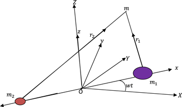
Figure 1. Configuration of the synodic coordinate system for the R3BP, where  , and
, and  are the triaxial primary, oblate secondary, and massless bodies, respectively.
Download figure:
Standard image High-resolution imageProceeding as elaborated in Singh & Begha (2011), we have solved numerically the above equation for different values of the parameters of the problem, and three such points have been found to exist in the intervals 
 , and
, and  named
named  , and
, and  respectively (see Szebehely 1967). Ten such cases are shown in Table 1, while the effect of the oblateness factor of the secondary, the influence of the Coriolis and centrifugal forces, and the effect of the triaxiality coefficients of the primary on the location of the collinear libration points can be seen in Figures 2 and 3.

Figure 2. Effects of the triaxiality coefficients of the more massive body on the positions of the equilibrium points  ,
,  , and
, and  The values of the remaining parameters are given in the first case of Table 1.
Download figure:
Standard image High-resolution image
Figure 3. Combined effects of the oblateness of the secondary body and perturbation in the centrifugal force on the positions of the equilibrium points  ,
,  , and
, and  The values of the remaining parameters are given in the first case of Table 1.
Download figure:
Standard image High-resolution imageTable 1.
Collinear Equilibrium Points for 
| Case |

|

|

|

|

|

|

|

|
|---|---|---|---|---|---|---|---|---|
| 1 | 0.000139 | 0.000132 | 0.000438 | 0.000145 | 0.000089 | −1.19341894 | −0.78314148 | 1.01033937 |
| 2 | 0.000339 | 0.000332 | 0.000638 | 0.000345 | 0.000289 | −1.19377095 | −0.78263393 | 1.01017634 |
| 3 | 0.000539 | 0.000532 | 0.000838 | 0.000545 | 0.000489 | −1.19411811 | −0.78223354 | 1.01001350 |
| 4 | 0.000739 | 0.000732 | 0.001038 | 0.000745 | 0.000689 | −1.19446057 | −0.78179005 | 1.00985086 |
| 5 | 0.000939 | 0.000932 | 0.001238 | 0.000945 | 0.000889 | −1.19479844 | −0.78135323 | 1.00968842 |
| 6 | 0.001139 | 0.001132 | 0.001438 | 0.001145 | 0.001089 | −1.19513186 | −0.78092285 | 1.00952617 |
| 7 | 0.001339 | 0.001332 | 0.001638 | 0.001345 | 0.001289 | −1.19546094 | −0.78049870 | 1.00936411 |
| 8 | 0.001539 | 0.001532 | 0.001838 | 0.001545 | 0.001489 | −1.19578579 | −0.78008057 | 1.00920224 |
| 9 | 0.001739 | 0.001732 | 0.002038 | 0.001745 | 0.001689 | −1.19610652 | −0.77966829 | 1.00904057 |
| 10 | 0.001939 | 0.001932 | 0.002238 | 0.001945 | 0.001889 | −1.19642323 | −0.77926165 | 1.00887910 |
Download table as: ASCIITypeset image
4. MOTION AROUND THE COLLINEAR EQUILIBRIUM POINTS
We define a new coordinate system whereby  is any collinear equilibrium point
  and is also the origin with
  ,
,  ,
,  as axes parallel to
  ,
,  , and
, and  , respectively. The relations that show the proper transformation between the two systems are

By the transformation of Equations (2) with the use of Equation (5) in the  coordinate system and expanding the right-hand side of the result obtained by Taylor series up to the second-order terms, we have


where
Also,  and
and  represent the signs of
  and
and  at any equilibrium point, thus avoiding the absolute values for each case.
4.1. Coplanar Periodic Orbits: Second-order Analysis and Numerical Investigation
4.1.1. Semianalytical Approximation of the 2D Periodic Orbits
For the planar case, we set in Equation (6)  and look for periodic solutions of the following system:
We consider that the sought solution in powers of an orbital parameter 
 is of the following form:

Substituting Equation (8) into the first and second equations represented in Equation (7) and equating the coefficients of the same powers of  , we obtain the following two systems:
and
respectively, which must be solved successively. The periodic solution of the linear system represented in Equations (9) is

where  is the period of the periodic orbit. Since
  and
and  are linearly independent functions, we equate their coefficients obtaining
and
respectively. Systems (12) and (13) are linear homogeneous, and for nonzero solutions the determinant must be zero, i.e.,
Note here that the roots of Equation (14) may determine the stability of the collinear equilibrium points since this equation coincides with the characteristic polynomial of the linearized system around a collinear equilibrium point. According to Lyapunov's theorem, the condition for stability is that if all four roots of Equation (14) are either negative real numbers or pure imaginary at each one of the collinear equilibrium points, then these are stable; otherwise, they are unstable. Thus, as can be seen from the results presented in Table 2, the collinear equilibria  are unstable for all the considered cases of Table 1.
Table 2. Roots of the Characteristic Equation (14) Determining the Stability of the Collinear Equilibrium Points
| Case |

|

|

|
|---|---|---|---|
| 1 | ±1.80634639, ±2.07999304i | ±2.41487845, ±3.08204901i | ±1.02180951, ±0.25679352i |
| 2 | ±1.80590282, ±2.08686171i | ±2.41481407, ±3.09176844i | ±1.02230697, ±0.25693104i |
| 3 | ±1.80549159, ±2.09362688i | ±2.41584384, ±3.10300319i | ±1.02280445, ±0.25706865i |
| 4 | ±1.80511129, ±2.10029188i | ±2.41635369, ±3.11312815i | ±1.02379938, ±0.25734358i |
| 5 | ±1.80476092, ±2.10686046i | ±2.41688023, ±3.12303243i | ±1.02379938, ±0.25734358i |
| 6 | ±1.80443918, ±2.11333558i | ±2.41742239, ±3.13272555i | ±1.02429686, ±0.25748107i |
| 7 | ±1.80414510, ±2.11972048i | ±2.41797929, ±3.14221666i | ±1.02479435, ±0.25761862i |
| 8 | ±1.80387770, ±2.12601817i | ±2.41854998, ±3.15151405i | ±1.02529186, ±0.25775623i |
| 9 | ±1.80363599, ±2.13223142i | ±2.41913390, ±3.16062614i | ±1.02578936, ±0.25789372i |
| 10 | ±1.80341912, ±2.13836300i | ±2.41972999, ±3.16955989i | ±1.02628684, ±0.25803108i |
Download table as: ASCIITypeset image
Since systems (12) and (13) are indeterminate, we arbitrarily choose  and
and  such that

Therefore, the periodic solution of Equations (9) is

Similarly, for Equations (10) we set
and working as previously, we find that

and

Thus, the periodic solution of Equations (10) is
Therefore, the sought periodic solution represented in Equations (8) into series expansions of the orbital parameter  up to second-order terms is
where  is the position of any collinear equilibrium point, while the coefficients
  are defined by Equations (15) and (18) and
  is a real positive solution of Equation (14).
In Figure 4, we present the families of planar symmetric periodic orbits, in their projection into  around all the collinear equilibrium points as they are computed by the first-order (red curve) and second-order (blue curve) analyses obtained in Equations (19), for
  and certain values of the orbital parameter
  We also show, in this figure, the accurate numerical solution (black curve) of the corresponding families obtained by the numerical integration of the full equations of motion (1). At each equilibrium point, we observe that the second-order semianalytical solution is always a better approximation of the numerical solution than the first one; the validity of our analysis is obvious.
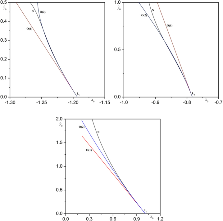
Figure 4. Comparison of the first-order (red curve, O(1)) and second-order (blue curve, O(2)) analyses, obtained from solution (19), with the corresponding numerical solution (black curve, N), obtained from the numerical integration of the full equations of motion (1), for all families of 2D periodic orbits emanating from the collinear equilibrium points.
Download figure:
Standard image High-resolution image4.1.2. Numerical Results for 2D Periodic Orbits
All families of planar symmetric periodic orbits emanating from the three collinear equilibrium points have been determined accurately by means of well-known differential corrections–predictions procedures based on the periodicity conditions

where  is the orbit's period. The above conditions ensure that the orbit in question will be also symmetric with respect to the Ox-axis. For appropriate initial conditions of the first member of each family we have used the second-order analysis of the previous subsection. In Tables 3–5, we give initial conditions for the Lyapunov families in all 10 cases of Table 1, i.e., for the corresponding 10 combinations of the parameters of the problem. The presented initial conditions correspond to the first accurate computed member of each family, i.e., the "almost" infinitesimal orbit around each collinear equilibrium point. In these tables, we give the values
  and
and  at
at  the value of the Jacobi constant C, the half period of the Lyapunov orbit, and the stability parameters as they were discussed in Section 2. We observe that, as in the classical problem, all the Lyapunov families start with unstable members due to the unstable nature of the collinear points.
Table 3.
Initial Conditions for the Lyapunov Family Emanating from  (Family A) for
| Case |

|

|
C | T/2 |

|

|
|---|---|---|---|---|---|---|
| 1 | −0.78320335 | 0.00055761 | 3.29220658 | 1.30093233 | 1519.17680 | 0.996137 |
| 2 | −0.78268995 | 0.00005442 | 3.29378966 | 1.30067713 | 1559.19297 | 0.998573 |
| 3 | −0.78223919 | 0.00005131 | 3.29536756 | 1.30041216 | 1599.13647 | 0.999801 |
| 4 | −0.78179535 | 0.00004826 | 3.29694067 | 1.30013776 | 1639.00392 | 0.999921 |
| 5 | −0.78135818 | 0.00004527 | 3.29850912 | 1.29985454 | 1678.79019 | 0.999023 |
| 6 | −0.78092747 | 0.00004235 | 3.30007301 | 1.29956303 | 1718.49045 | 0.997190 |
| 7 | −0.78050299 | 0.00003949 | 3.30163246 | 1.29926375 | 1758.10049 | 0.994501 |
| 8 | −0.78013438 | 0.00049669 | 3.30318738 | 1.29895731 | 1797.61312 | 0.991025 |
| 9 | −0.77972163 | 0.00049393 | 3.30473827 | 1.29864382 | 1837.03001 | 0.986829 |
| 10 | −0.77926502 | 0.00003124 | 3.30628524 | 1.29832380 | 1876.34888 | 0.981973 |
Download table as: ASCIITypeset image
Table 4.
Initial Conditions for the Lyapunov Family Emanating from  (Family B) for
| Case |

|

|
C | T/2 |

|

|
|---|---|---|---|---|---|---|
| 1 | 1.00990049 | 0.00089774 | 3.02662588 | 3.07453847 | 2.52824 | 0.998159 |
| 2 | 1.00998200 | 0.00039769 | 3.02764766 | 3.07304255 | 2.52842 | 0.998243 |
| 3 | 1.00981929 | 0.00039763 | 3.02866935 | 3.07154790 | 2.52860 | 0.998324 |
| 4 | 1.00965677 | 0.00039758 | 3.02969113 | 3.07005469 | 2.52878 | 0.998404 |
| 5 | 1.00949445 | 0.00039753 | 3.03071298 | 3.06856292 | 2.52896 | 0.998481 |
| 6 | 1.00933232 | 0.00039748 | 3.03173493 | 3.06707258 | 2.52913 | 0.998557 |
| 7 | 1.00917039 | 0.00039743 | 3.03275695 | 3.06558367 | 2.52931 | 0.998630 |
| 8 | 1.00900864 | 0.00039738 | 3.03377906 | 3.06409619 | 2.52949 | 0.998702 |
| 9 | 1.00884709 | 0.00039733 | 3.03480125 | 3.06261014 | 2.52966 | 0.998772 |
| 10 | 1.00868574 | 0.00039728 | 3.03582352 | 3.06112551 | 2.52984 | 0.998840 |
Download table as: ASCIITypeset image
Table 5.
Initial Conditions for the Lyapunov Family Emanating from  (Family C) for
| Case |

|

|
C | T/2 |

|

|
|---|---|---|---|---|---|---|
| 1 | −1.19346066 | 0.00021533 | 3.25850958 | 1.73919728 | 693.59589 | 0.981461 |
| 2 | −1.19381226 | 0.00021386 | 3.26024175 | 1.73962442 | 711.63449 | 0.987381 |
| 3 | −1.19415903 | 0.00021240 | 3.26197253 | 1.74002068 | 729.79313 | 0.992083 |
| 4 | −1.19450109 | 0.00021097 | 3.26370196 | 1.74038723 | 748.06923 | 0.995633 |
| 5 | −1.19483859 | 0.00020955 | 3.26543006 | 1.74072516 | 766.46027 | 0.998096 |
| 6 | −1.19517354 | 0.00021815 | 3.26715689 | 1.74103552 | 784.96375 | 0.999533 |
| 7 | −1.19550034 | 0.00020678 | 3.26888247 | 1.74131928 | 803.57732 | 1.000000 |
| 8 | −1.19582483 | 0.00020542 | 3.27060684 | 1.74157740 | 822.29857 | 0.999553 |
| 9 | −1.19615279 | 0.00024407 | 3.27233001 | 1.74181079 | 841.12520 | 0.998245 |
| 10 | −1.19646535 | 0.00022275 | 3.27405205 | 1.74202027 | 860.05505 | 0.996124 |
Download table as: ASCIITypeset image
The graphical representation of the evolution of the orbits of the families emanating from all collinear equilibrium points is shown in Figure 5. In particular, in the first frame of this figure, we present the evolution of periodic orbits of family A emanating from the equilibrium point  in the second frame we show the evolution of periodic orbits of family B emanating from
  while the evolution of periodic orbits of family C emanating from the collinear point
  is shown in the third frame. In the last frame, the family characteristics, in the space of initial conditions
  are presented, together with the forbidden regions to the motion of the massless body. In Figure 6, we show the horizontal and vertical stability curves of the corresponding Lyapunov families. Note that, due to the large values of the stability indices, we plot
  instead of
  and
and  instead of
  (except for the last frame); therefore, the inequalities
  and
and  for stability become in this case
  and
and  respectively. As we observe, all families consist of horizontally and vertically stable parts, except for the Lyapunov family emanating from
  , which is horizontally unstable.

Figure 5. Evolution of the orbits of the Lyapunov families A, B, and C emanating from  ,
,  , and
, and  for case 1 of Tables 3, 4, and 5, respectively. The last frame presents the respective family characteristics, together with the forbidden regions to the motion of the massless body in the space of initial conditions.
Download figure:
Standard image High-resolution image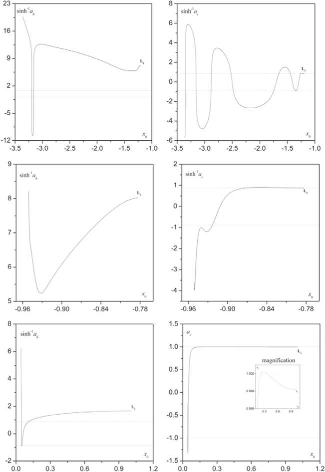
Figure 6. Horizontal and vertical stability curves (left and right frames, respectively) of the Lyapunov families emanating from the collinear equilibrium points  , and
, and  corresponding to case 1 of Tables 5, 3, and 4, respectively. Vertical stability exists for all the Lyapunov families.
Download figure:
Standard image High-resolution image4.2. Spatial Periodic Orbits: Second-order Analysis and Numerical Investigation
4.2.1. Semianalytical Approximation of the 3D Periodic Orbits
We consider now that the sought solution of Equation (6) in powers of the orbital parameter  is of the following form:

Putting the last equations into Equation (6) and equating the coefficients of the same powers of  , we find
and

Setting in Equation (22)  , we find that
  , which has a nonzero solution only when
  . Additionally, by setting
and working as was done previously in the planar case, we find that the solution of Equations (21) is


where


While  ,
,  . Therefore, the periodic solution up to second-order terms w.r.t. the orbital parameter
  is
is
To establish the validity of our analysis, we present in Figure 7, as an example, the projections of the semianalytical solution of Equations (26) about the collinear equilibrium point  in the
  and
and  planes (blue curves), for
  and a certain range of values of the orbital parameter
  together with the corresponding accurate numerical solution (black curves) obtained by the numerical integration of the equations of motion (1).

Figure 7. Comparison, in the space of initial conditions, of the semianalytical solution (blue curve denoted by A) obtained by our analysis and the corresponding numerical solution (black curve denoted by N) obtained by the numerical integration of the equations of motion, in the case of the family of 3D periodic orbits emanating from the collinear equilibrium point 
Download figure:
Standard image High-resolution image4.2.2. Numerical Results for 3D Periodic Orbits
In order to compute numerically the first member of a family of 3D periodic orbits emanating from any collinear equilibrium point, we have used the approximate solution of Equations (26) for appropriate initial conditions. We then applied well-known predictor–corrector schemes based on the periodicity conditions:
so as to obtain the whole family. Note that T is the period of a 3D periodic orbit; we seek periodicity conditions at the quarter of the period due to the double symmetry of the orbits in question with respect to the Ox-axis and Oxz-plane.
In Tables 6–8, we present initial conditions for all the computed families of 3D periodic orbits emanating from the collinear equilibrium points, for cases 1–10 of Table 1. In each table, we give the values of  , and
, and  (since
  for double symmetry w.r.t. the Ox-axis and Oxz-plane), the value of the Jacobi constant
  the quarter of the orbit's period T/4, and the stability parameters
  and
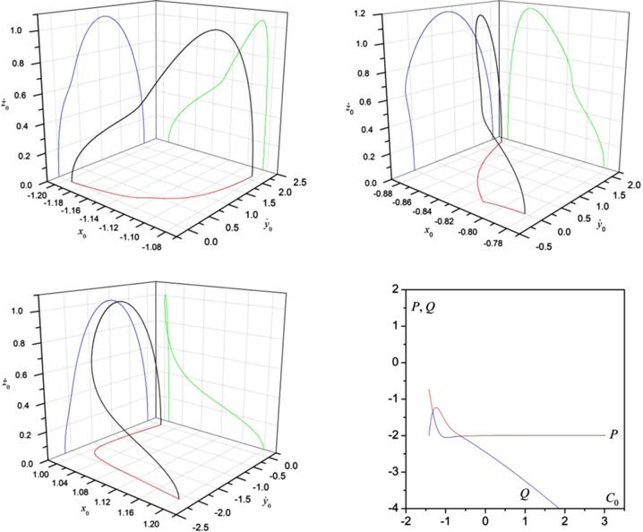
and  as discussed in Section 2 (see also Hénon 1973, for details). In Figure 8, we show the evolution of the characteristic curves of the respective families in the space of initial conditions
  As we see, all the computed families emanate from the corresponding equilibrium point and terminate at a planar periodic orbit. Only family B emanating from the equilibrium point
  possesses stable parts, and this is shown in the last frame of Figure 8.
Figure 8. Characteristic curves of the families C, A, and B (first, second, and third frame, respectively) of 3D periodic orbits (produced by the initial conditions given in case 1 of Tables 6–8), together with their corresponding projections, emanating from the collinear equilibrium points. Only family B emanating from  contains stable parts; its stability is shown in the last frame.
Download figure:
Standard image High-resolution image
Table 6.
Initial Conditions for the Family of 3D Periodic Orbits Emanating from  (Family A) for
| Case |

|

|

|
C | T/4 |

|

|
|---|---|---|---|---|---|---|---|
| 1 | −0.78371825 | −0.00100520 | 0.07000000 | 3.28730991 | 0.66255038 | −1.98864 | −3314.05 |
| 2 | −0.78326989 | −0.00100980 | 0.07000000 | 3.28889287 | 0.65878156 | −1.99500 | −3250.13 |
| 3 | −0.78282805 | −0.00101365 | 0.07000000 | 3.29047091 | 0.65514644 | −1.99881 | −3190.09 |
| 4 | −0.78239255 | −0.00101681 | 0.07000000 | 3.29204416 | 0.65163732 | −2.00032 | −3133.60 |
| 5 | −0.78196317 | −0.00101938 | 0.07000000 | 3.29361273 | 0.64824705 | −1.99977 | −3080.36 |
| 6 | −0.78153975 | −0.00102140 | 0.07000000 | 3.29517676 | 0.64496907 | −1.99739 | −3030.09 |
| 7 | −0.78112209 | −0.00102294 | 0.07000000 | 3.29673634 | 0.64179726 | −1.99334 | −2982.55 |
| 8 | −0.78071003 | −0.00102406 | 0.07000000 | 3.29829158 | 0.63872594 | −1.98782 | −2937.54 |
| 9 | −0.78030340 | −0.00102478 | 0.07000000 | 3.29984259 | 0.63574986 | −1.98098 | −2894.84 |
| 10 | −0.77990206 | −0.00102516 | 0.07000000 | 3.30138946 | 0.63286412 | −1.97296 | −2854.29 |
Download table as: ASCIITypeset image
Table 7.
Initial Conditions for the Family of 3D Periodic Orbits Emanating from  (Family B) for
| Case |

|

|

|
C | T/4 |

|

|
|---|---|---|---|---|---|---|---|
| 1 | 1.01031202 | 0.00240785 | 0.07000000 | 3.02172030 | 1.55226617 | 1.99624 | −5.12362 |
| 2 | 1.01014834 | 0.00240716 | 0.07000000 | 3.02274191 | 1.55116450 | 1.99641 | −5.12229 |
| 3 | 1.00998484 | 0.00240647 | 0.07000000 | 3.02376361 | 1.55006420 | 1.99658 | −5.12096 |
| 4 | 1.00982155 | 0.00240578 | 0.07000000 | 3.02478539 | 1.54896525 | 1.99674 | −5.11963 |
| 5 | 1.00965845 | 0.00240509 | 0.07000000 | 3.02580725 | 1.54786765 | 1.99690 | −5.11830 |
| 6 | 1.00949555 | 0.00240440 | 0.07000000 | 3.02682919 | 1.54677141 | 1.99705 | −5.11698 |
| 7 | 1.00933284 | 0.00240371 | 0.07000000 | 3.02785122 | 1.54567652 | 1.99720 | −5.11565 |
| 8 | 1.00917032 | 0.00240301 | 0.07000000 | 3.02887333 | 1.54458298 | 1.99735 | −5.11433 |
| 9 | 1.00900800 | 0.00240232 | 0.07000000 | 3.02989552 | 1.54349082 | 1.99749 | −5.11301 |
| 10 | 1.00884588 | 0.00240162 | 0.07000000 | 3.03091780 | 1.54239994 | 1.99763 | −5.11169 |
Download table as: ASCIITypeset image
Table 8.
Initial Conditions for the Family of 3D Periodic Orbits Emanating from  (Family C) for
| Case |

|

|

|
C | T/4 |

|

|
|---|---|---|---|---|---|---|---|
| 1 | 1.19234688 | 0.00243426 | 0.07000000 | 3.25361184 | 0.89811482 | 1.95337 | −1696.37 |
| 2 | 1.19268616 | 0.00242876 | 0.07000000 | 3.25534427 | 0.89339954 | 1.96743 | −1669.89 |
| 3 | 1.19302125 | 0.00242284 | 0.07000000 | 3.25707531 | 0.88881356 | 1.97871 | −1644.76 |
| 4 | 1.19335225 | 0.00241655 | 0.07000000 | 3.25880499 | 0.88435105 | 1.98741 | −1620.87 |
| 5 | 1.19367926 | 0.00240993 | 0.07000000 | 3.26053335 | 0.88000653 | 1.99374 | −1598.15 |
| 6 | 1.19400236 | 0.00240304 | 0.07000000 | 3.26226042 | 0.87577481 | 1.99788 | −1576.52 |
| 7 | 1.19432165 | 0.00239591 | 0.07000000 | 3.26398624 | 0.87165103 | 1.99999 | −1555.89 |
| 8 | 1.19463720 | 0.00238858 | 0.07000000 | 3.26571085 | 0.86763058 | 2.00024 | −1536.20 |
| 9 | 1.19494911 | 0.00238107 | 0.07000000 | 3.26743426 | 0.86370912 | 1.99877 | −1517.40 |
| 10 | 1.19525744 | 0.00237341 | 0.07000000 | 3.26915653 | 0.85988255 | 1.99571 | −1499.42 |
Download table as: ASCIITypeset image
5. DISCUSSION AND CONCLUSIONS
A generalization of the R3BP where the larger primary is a triaxial rigid body and the smaller one is an oblate body was considered. Specifically, the effects of triaxiality and oblateness, together with small perturbations in the Coriolis and centrifugal forces, were investigated to the positions of the collinear equilibrium points. In 10 studied cases of the parameters of the problem, it was found that the positions of the collinear equilibrium points  and
and  move toward the origin with the increase of the values of these parameters, while the equilibrium point
  moves away from the origin. It was also shown that the three collinear equilibrium points are unstable in all the considered cases. Note here that, in the case where one or both primaries are prolate bodies or sources of radiation, it has been found that these points may be stable (see, e.g., Douskos et al. 2012; Perdios et al. 2015).
The infinitesimal periodic orbits around the collinear equilibrium points were also determined. To this purpose, semianalytical solutions were constructed in both 2D and 3D cases. In addition, the numerical continuation of the families of planar and spatial periodic orbits emanating from the collinear equilibria was established. As in the classical R3BP, all the computed families of 2D periodic orbits go to collision orbits with the primaries, while the corresponding families of 3D periodic orbits terminate at bifurcations with planar periodic orbits. It was found that only the planar Lyapunov families emanating from the collinear equilibria  and
and  may contain horizontally stable orbits, but all these families may contain parts with vertically stable orbits. Similar behavior for the planar Lyapunov families when the larger primary is a source of radiation has also been observed by Ragos & Zagouras (1991), who found that only the Lyapunov family emanating from the outer collinear equilibrium point to the left of the larger primary may contain horizontally stable orbits. For the triaxial secondary body Jain et al. (2006) obtained only unstable planar Lyapunov orbits for all the collinear equilibrium points. Finally, we found that in the 3D case only the corresponding family emanating from
  may consist of stable periodic orbits, and this is in agreement with the results presented by Tsirogiannis et al. (2006) in the framework of the R3BP with the larger primary being a radiation source and the smaller one being an oblate spheroid.