Binding Energies of Interstellar Molecules on Crystalline and Amorphous Models of Water Ice by Ab Initio Calculations

Stefano Ferrero; Lorenzo Zamirri; Cecilia Ceccarelli; Arezu Witzel; Albert Rimola; Piero Ugliengo

doi:10.3847/1538-4357/abb953

1. Introduction

The presence of molecules in the extreme physical conditions of the interstellar medium (ISM) was considered impossible by astronomers, until the first diatomic species (CN, CH, and CH⁺) were detected in the ISM from optical and ultraviolet transitions (Swings & Rosenfeld 1937; McKellar 1940; Douglas & Herzberg 1942). Nowadays more than 200 gaseous molecular species (including radicals and ions) have been identified in the diffuse and dense regions of the ISM, thanks to their rotational and vibrational lines in the radio to far-infrared (FIR) wavelengths (e.g., see the review by McGuire 2018). In the coldest (≤20–90 K) and densest (≥10³ cm⁻³) ISM, some of these molecules are also detected in the solid state via near-infrared (NIR) observations (e.g., see the review by Boogert et al. 2015).

We now know that the solid-state molecules are frozen species that envelop the submicron dust grains that permeate the ISM and whose refractory core is made of silicates and carbonaceous materials (e.g., Jones 2013; Jones et al. 2017). The grain iced mantle composition is governed by the adsorption of species from the gas phase and by chemical reactions occurring on the grain surfaces. For example, the most abundant component of the grain mantles is H₂O, which is formed by the hydrogenation of O, O₂, and O₃ on the grain surfaces (e.g., Hiraoka et al. 1998; Dulieu et al. 2010; Oba et al. 2012).

The water-rich ice is recognized from two specific NIR bands at about 3 and 6 μm, which are associated with its O–H stretching and H–O–H bending modes, respectively (e.g., see the review by Boogert et al. 2015). In addition, species like CO, CO₂, NH₃, CH₄, CH₃OH, and H₂CO have also been identified as minor constituents of the ice mantles, which, for this reason, are sometimes referred to as "dirty ices" (Boogert et al. 2015). Furthermore, the comparison between the astronomical spectroscopic observations and the laboratory spectra of an analogous interstellar ice sample, principally based on the O–H stretching feature, has shown that the mantle ices very likely possess an amorphous-like structure resembling that of amorphous solid water (ASW; e.g., Watanabe & Kouchi 2008; Oba et al. 2009; Boogert et al. 2015).

Ice surfaces are known to have an important role in the interstellar chemistry because they can serve as catalysts for chemical reactions that cannot proceed in the gas phase, such as the formation of H₂, the most abundant molecule in the ISM (Hollenbach & Salpeter 1971). Ice surfaces can catalyze reactions by behaving as (i) a passive third body, this way absorbing part of the excess of energy released in the surface processes (adsorption and/or chemical reaction) (e.g., Pantaleone et al. 2020); (ii) a chemical catalyst, this way directly participating in the reaction reducing the activation energies (e.g., Rimola et al. 2018; Enrique-Romero et al. 2019, 2020); or (iii) a reactant concentrator, this way retaining the reactants and keeping them in close proximity for subsequent reaction (e.g., CO adsorption and retention for subsequent hydrogenation to form H₂CO and CH₃OH (e.g., Watanabe & Kouchi 2002; Rimola et al. 2014; Zamirri et al. 2019b). All three processes depend on the binding energies (BEs) of the molecules either directly (e.g., the adsorption of the species) or indirectly (e.g., because the diffusion of a particle on the grain surfaces is a fraction of its BE) (see Cuppen et al. 2017). In addition, molecules formed on the grain surfaces can be later transferred to the gas phase by various desorption processes, most of which depend, again, on the BE of the species. In practice, BEs are crucial properties of the interstellar molecules and play a huge role in the resulting ISM chemical composition. This key role of BEs is very obvious in the astrochemical models that aim at reproducing the chemical evolution of interstellar objects, as clearly shown by two recent works by Wakelam et al. (2017) and Penteado et al. (2017), respectively.

Experimentally, the BEs of astrochemical species are measured by temperature programmed desorption (TPD) experiments. These experiments measure the energy required to desorb a particular species from the substrate, namely, a desorption enthalpy, which is equal to the BE only if there are no activated processes (He et al. 2016) and if thermal effects are neglected. A typical TPD experiment consists of two phases. In the first one, the substrate, maintained at a constant temperature, is exposed to the species that have to be adsorbed coming from the gas phase. In the second phase, the temperature is increased until desorption of the adsorbed species—collected and analyzed by a mass spectrometer—occurs. The BE is then usually extracted by applying the direct inversion method on the Polanyi–Wigner equation (e.g., Dohnalek et al. 2001; Noble et al. 2012). The BE values obtained in this way strongly depend on the chemical composition and morphology of the substrate and also on whether the experiment is conducted in the monolayer or multilayer regime (e.g., Noble et al. 2012; He et al. 2016; Chaabouni et al. 2018). Another issue related to the TPD technique is that it cannot provide accurate BBEs for radical species, as they are very reactive. In the literature, there are many works that have investigated the desorption processes by means of the TPD technique (e.g., Collings et al. 2004; Noble et al. 2012; Dulieu et al. 2013; Fayolle et al. 2016; He et al. 2016; Smith et al. 2016), but they have been conducted for just a handful of important astrochemical species, whereas a typical network of an astrochemical model can contain up to 500 species and very different substrates. In a recent work, Penteado et al. (2017) collected the results of these experimental works, trying to be as homogeneous as possible in terms of different substrates, estimating the missing BE values from the available data and performing a systematic analysis on the effect that the BE uncertainties can have on astrochemical model simulations.

BE values can also be obtained by means of computational approaches that, in some situations, can overcome the experimental limitations. Many computational works have so far focused on a few important astrochemical species like H, H₂, N, O, CO, and CO₂, in which BEs are calculated on periodic/cluster models of crystalline/amorphous structural states using different computational techniques (e.g., Al-Halabi & Van Dishoeck 2007; Karssemeijer et al. 2014; Karssemeijer & Cuppen 2014; Ásgeirsson et al. 2017; Senevirathne et al. 2017; Shimonishi et al. 2018; Zamirri et al. 2019a). In addition, other works have computed BEs in a larger number of species but with a very approximate model of the substrate. For example, in a recent work by Wakelam et al. (2017) BE values of more than 100 species are calculated by approximating the ASW surface with a single water molecule. The authors then fitted the most reliable BE measurements (16 cases) against the corresponding computed ones, obtaining a good correlation between the two data sets. In this way, all the errors in the computational methods and limitations due to the adoption of a single water molecule are compensated by the fitting with the experimental values, in the view of the authors. The resulting parameters are then used to scale all the remaining computed BEs to improve their accuracy. This clever procedure does, however, consider the proposed scaling universal, leaving aside the complexity of the real ice surface and the specific features of the various adsorbates. In a similar work, Das et al. (2018) have calculated the BEs of 100 species by increasing the size of a water cluster from one to six molecules, noticing that the calculated BE approaches the experimental value when the cluster size is increased. As we will show in the present work, these approaches, relying on an arbitrary and very limited number of water molecules, cannot, however, mimic a surface of icy grain. Furthermore, the strength of interaction between icy water molecules, as well as with respect to the adsorbates, depends on the hydrogen bond cooperativity, which is underestimated in small water clusters.

In this work, we followed a different approach, focusing on extended periodic ice models, either crystalline or amorphous, adopting a robust computational methodology based on a quantum mechanical approach. We simulate the adsorption of a set of 21 interstellar molecules, 4 of which are radical species, on several specific exposed sites of the water surfaces of both extended models. BE values have been calculated for more than one binding site (if present) to provide the spread of the BE values that the same molecule can have depending on the position in the ice. Different approaches, with different computational cost, have been tested and compared, and the final computed BEs have been compared with data from the computational approaches of Wakelam et al. (2017) and Das et al. (2018) and data from UMIST and KIDA databases, as well as available experimental data (e.g., McElroy et al. 2013; Wakelam et al. 2015). One added value of this work is the definition of both a reliable, computationally cost-effective ab initio procedure designed to arrive at accurate BE values and an ice grain atomistic model that can be applied to predict the BEs of any species of astrochemical interest.

2. Computational Details

2.1. Structure of the Ice: Periodic Simulations

Water ice surfaces have been modeled enforcing periodic boundary conditions to define icy slabs of finite thickness either entirely crystalline or of amorphous nature. Adsorption is then carried out from the void region above the defined slabs. Periodic calculations have been performed with the ab initio CRYSTAL17 code (Dovesi et al. 2018). This software implements both the Hartree–Fock (HF) and Kohn–Sham self-consistent field methods for the solution of the electronic Schrödinger equation, fully exploiting, if present, the crystalline or molecular symmetry of the system under investigation. CRYSTAL17 adopts localized Gaussian functions as basis sets, similar to the approach followed by molecular codes. This allows CRYSTAL17 to perform geometry optimizations and vibrational properties of both periodic (polymer, surfaces, and crystals) and nonperiodic (molecules) systems with the same level of accuracy. Furthermore, the definition of the surfaces through the slab model allows us to avoid the 3D fake replica of the slab as forced when adopting the plane wave basis set.

Computational parameters are set to values ensuring good accuracy in the results. The threshold parameters for the evaluation of the Coulomb and exchange bi-electronic integrals (TOLINTEG keyword in the CRYSTAL17 code; Dovesi et al. 2018) have been set equal to 7, 7, 7, 7, and 14. The needed density functional integration is carried out numerically over a grid of points, which is based on an atomic partition method developed by Becke (1988). The standard pruned grid (XLGRID keyword in the CRYSTAL17 code; Dovesi et al. 2018), composed of 75 radial points and a maximum of 974 angular points, was used. The sampling of the reciprocal space was conducted with a Pack–Monkhorst mesh (Pack & Monkhorst 1977), with a shrinking factor (SHRINK in the code CRYSTAL17; Dovesi et al. 2018) of 2, which generates 4k points in the first Brillouin zone. The choice of the numerical values we assigned to these three computational parameters is fully justified in Appendix A.

Geometry optimizations have been carried out using the Broyden–Fletcher–Goldfarb–Shanno (BFGS) algorithm (Broyden 1970; Fletcher 1970; Goldfarb 1970; Shanno 1970), relaxing both the atomic positions and the cell parameters. We adopted the default values for the parameters controlling the convergence, i.e., difference in energy between two subsequent steps, 1 × 10⁻⁷ Hartree; and maximum components and rms of the components of the gradients and atomic displacement vectors, 4.5 × 10⁻⁴ hartrees bohr⁻¹ and 3 × 10⁻⁴ hartrees bohr⁻¹, and 1.8 × 10⁻³ bohr and 1.2 × 10⁻³ bohr, respectively. All periodic calculations were grounded on either the density functional theory (DFT) or the HF-3c method (Hohenberg & Kohn 1964; Sure & Grimme 2013). Within the DFT framework, different functionals were used to describe closed- and open-shell systems. For the former, we used the hybrid B3LYP method (Lee et al. 1988; Becke 1993), which has been shown to provide a good level of accuracy for the interaction energies of noncovalent bound dimers (Kraus & Frank 2018), added with the D3-BJ correction for the description of dispersive interactions (Grimme et al. 2010, 2011). For open-shell systems, treated with a spin-unrestricted formalism (Pople et al. 1995), we used the hybrid M06-2X functional (Zhao & Truhlar 2008), which has been proved to give accurate results in estimating the interaction energy of noncovalent binary complexes involving a radical species and a polar molecule (Tentscher & Arey 2013). The choice of these two different functionals is justified by two previous works describing the accuracy on the energetic properties of molecular adducts (Tentscher & Arey 2013; Kraus & Frank 2018). For all periodic DFT calculations we used the Ahlrichs triple-zeta quality VTZ basis set, supplemented with a double set of polarization functions (Schäfer et al. 1992). In the following, we will refer to this basis set as "A-VTZ*" (see Appendix D for details of the adopted basis set).

The HF-3c method is a new method combining the Hartree–Fock Hamiltonian with the minimal basis set MINI-1 (Tatewaki & Huzinaga 1980) and with three a posteriori corrections for (i) the basis set superposition error (BSSE), arising when localized Gaussian functions are used to expand the basis set (Jansen & Ros 1969; Liu & McLean 1973); (ii) the dispersive interactions; and (iii) short-ranged deficiencies due to the adopted minimal basis set (Sure & Grimme 2013).

Harmonic frequency calculations were carried out on the optimized geometries of both crystalline and amorphous ices to characterize the stationary points of each structure. Vibrational frequencies have been calculated at the Γ point by diagonalizing the mass-weighted Hessian matrix of second-order energy derivatives with respect to atomic displacements (Pascale et al. 2004; Zicovich-Wilson et al. 2004). The Hessian matrix elements have been evaluated numerically by a six-point formula (NUMDERIV = 2 in the CRYSTAL17 code; Dovesi et al. 2018), based on two displacements of ±0.001 Å for each nuclear Cartesian coordinate from the minimum structure.

To avoid computational burden, only a portion of the systems has been considered in the construction of the Hessian matrix, including the adsorbed species and the spatially closest interacting water molecules of the ice surface. This "fragment" strategy for the frequency calculation has already been tested by some of us in previous works and is fully justified by the noncovalent nature of the interacting systems, where the coupling between the vibrational modes of bulk ice and adsorbate moieties is negligible (Tosoni et al. 2005; Rimola et al. 2008; Zamirri et al. 2017).

From the set of frequencies resulting from the "fragment" calculations we worked out the zero-point energy (ZPE) for the free crystalline ice surface, the free adsorbate, and the ice surface/adsorbate complex to arrive at the corresponding correction ΔZPE, as reported in Appendix A.1. From the ΔZPE we corrected the electronic BE for each adsorbate as BE(0) = BE − ΔZPE and found a good linear correlation BE(0) = 0.854 BE, as shown in Appendix A.1. While the "fragment frequency" strategy is fine for computing the ΔZPE of the crystalline ice model owing to the structural rigidity enforced by the system symmetry, the same does not hold for the amorphous ice. In that case, the large unit cell (60 water molecules) and their random organization render the ice structure rather sensitive to the adsorbate interaction, which causes large structural water molecule rearrangement. This, in turn, alters significantly the whole set of normal modes, and the numerical value of the ΔZPE becomes ill-defined. Nevertheless, considering that the kinds of interactions operative for the crystal ice are of the same nature as those for the amorphous one, we adopted the same scaling factor of 0.854 computed for the crystalline ice to correct the electronic BE for the amorphous one. In the following, we compared the experimental BE usually measured for amorphous ices with the BE(0) values. To discuss the internal comparison between adsorption features of different adsorbates on the crystalline ice, we still focused on the uncorrected BEs.

2.2. BE Calculation and Counterpoise Correction

When Gaussian basis sets are used, a spurious contribution arises in the calculation of the molecule/surface interactions, called the BSSE (e.g., Boys & Bernardi 1970). In this work, the BSSE for DFT calculations has been corrected making use of the a posteriori counterpoise (CP) correction by Boys and Bernardi (Davidson & Feller 1986). The CP-corrected interaction ΔE^CP energy has been calculated as

$\begin{eqnarray}&&{\rm{\Delta }}{E}^{\mathrm{CP}}={\rm{\Delta }}E* +\delta E+{\rm{\Delta }}{E}_{L}-\mathrm{BSSE}\end{eqnarray} \tag{ 1 }$

where ${\rm{\Delta }}E*$ is the deformation-free interaction energy, δE is the total contribution to the deformation energy, and ΔE_L is the lateral interaction (adsorbate−adsorbate interaction) energy contribution. Details on the calculation of each energetic term of Equation (1) can be found in Appendix A. By definition, BE is the opposite of the CP-corrected interaction energy:

$\begin{eqnarray}&&{\rm{\Delta }}{E}^{\mathrm{CP}}=-\mathrm{BE}.\end{eqnarray} \tag{ 2 }$

2.3. BE Refinement with the Embedded Cluster Method

With the aim of refining the periodic DFT BE values for the crystalline ice model, single-point energy calculations have been carried out on small clusters, cut out from the crystalline ice model, using a higher level of theory than the DFT methods with the Gaussian09 program (Frisch et al. 2009). The adopted cluster models were derived from the periodic systems and are described in Section 3.2.2. These refinements have been performed through the ONIOM2 approach (Dapprich et al. 1999), dividing the systems into two parts that are described by two different levels of theory. The Model system (i.e., a small moiety of the whole system, including the adsorbate and the closest water molecules) was described by the High level of theory represented by the single- and double-electronic excitation coupled-cluster method with an added perturbative description of triple excitations (CCSD(T)). The Real system (i.e., the whole system) was described by the DFT level of theory adopted in the periodic calculations with the two different functionals for open- and closed-shell species. In the ONIOM2 methodology, the BE can be written as

$\begin{eqnarray}&&\mathrm{BE}(\mathrm{ONIOM}2)=-\mathrm{BE}(\mathrm{Low},\mathrm{Real})+{\rm{\Delta }}\mathrm{BE}\end{eqnarray} \tag{ 3 }$

$\begin{eqnarray}&&{\rm{\Delta }}\mathrm{BE}=\mathrm{BE}(\mathrm{High},\mathrm{Model})-\mathrm{BE}(\mathrm{Low},\mathrm{Model}).\end{eqnarray} \tag{ 4 }$

The final BE(ONIOM2) is also corrected by the BSSE following the same scheme described above. Our choices about the Model and Real systems will be extensively justified in Section 3.2.2.

3. Results

3.1. Ice Surface Models

3.1.1. Crystalline Ice Model

Despite the amorphous and perhaps porous nature of the interstellar ice, we adopted, as a paradigmatic case, a proton-ordered crystalline bulk ice model usually known as P-ice (Pna2₁ space group; Casassa et al. 1997). From P-ice bulk, we cut out a slab model, i.e., a 2D-periodic model representing a surface. Consequently, periodic boundary conditions are maintained only along the two directions defining the slab plane, while the third direction (z-axis) is nonperiodic and defines the slab thickness. The slab model adopted in this work represents the P-ice (010) surface, in accordance with previous work (Zamirri et al. 2018). This slab consists of 12 atomic layers, is stoichiometric, and has a null electric dipole moment across the z-axis. This ensures an electronic stability of the model with the increase of the slab thickness (Tasker 1979). The slab structure has been fully optimized (unit cell and atomic fractional coordinates) at both B3LYP-D3/A-VTZ* and M06-2X/A-VTZ* DFT levels. As can be seen from Figure 1 (panel (a)), the (010) P-ice unit cell is rather small, showing only one dangling hydrogen (dH) and oxygen (dO) as binding sites. For large molecules, to increase the number of adsorption sites and minimize the lateral interactions among replicas of the adsorbate, we also considered a 2 × 1 supercell. The electrostatic potential maps (EPMs; see Figure 1, panels (b) and (c)) clearly reveal positive (blue EPM regions) and negative (red EPM regions) potentials around the dH and dO sites, respectively.

**Figure 1.** The (010) slab model of P-ice. (a) Side view along the ${\boldsymbol{b}}$ lattice vector. (b) Top view of the 1 × 1 unit cell ( $| {\boldsymbol{a}}|$ = 4.500 Å and $| {\boldsymbol{b}}|$ = 7.078 Å) superimposed onto the EPM. (c) Top view of the 2 × 1 supercell ( $| {\boldsymbol{a}}|$ = 8.980 Å, $| {\boldsymbol{b}}|$ = 7.081 Å) superimposed onto the EPM. The isosurface value for the electron density where the electrostatic potential is mapped is set equal to 10⁻⁶ au. Color code: +0.02 au (blue, positive), 0.00 au (green, neutral), and −0.02 au (red, negative).
Download figure:
Standard image High-resolution image

**Figure 1.** The (010) slab model of P-ice. (a) Side view along the ${\boldsymbol{b}}$ lattice vector. (b) Top view of the 1 × 1 unit cell ( $| {\boldsymbol{a}}|$ = 4.500 Å and $| {\boldsymbol{b}}|$ = 7.078 Å) superimposed onto the EPM. (c) Top view of the 2 × 1 supercell ( $| {\boldsymbol{a}}|$ = 8.980 Å, $| {\boldsymbol{b}}|$ = 7.081 Å) superimposed onto the EPM. The isosurface value for the electron density where the electrostatic potential is mapped is set equal to 10⁻⁶ au. Color code: +0.02 au (blue, positive), 0.00 au (green, neutral), and −0.02 au (red, negative).
Download figure:
Standard image High-resolution image

3.1.2. Amorphous Solid Water (ASW)

As anticipated, the (010) P-ice surface might not be a physically sound model to represent actual interstellar ice surfaces, due to the evidence, from the spectroscopic feature of the interstellar ice, of its amorphous nature (Boogert et al. 2015). The building up of amorphous surface models is a nontrivial and not unique procedure, because of the lack of a consistent and universally accepted strategy. One common approach is to start from a crystalline model and heat it up to relatively high temperature by running molecular dynamics (MD) simulations for a few picoseconds. This step is followed by thermal annealing to freeze the ice in a glassy amorphous state. In this work, we adopted a different strategy. We refer to a recent work by Shimonishi et al. (2018) in which the BEs of a set of atomic species were computed on several water clusters, previously annealed with MD simulations. We reoptimized (at the B3LYP-D3/A-VTZ* level only) the whole set of ice clusters, and the three most stable clusters, composed of 20 water molecules each, were merged together to define a unit cell of an amorphous periodic ice. This procedure mimics somehow the collision of nanometric-scale icy grains occurring in the molecular clouds. The merger of the three clusters was carried out by matching the dH regions of one cluster with the dO ones of the other. As a result, we ended up with a large 3D-periodic unit cell (with lattice parameters $| {\boldsymbol{a}}|$ = 21.11 Å, $| {\boldsymbol{b}}|$ = 11.8 Å, and $| {\boldsymbol{c}}|$ = 11.6 Å) envisaging 60 water molecules. This initial bulk model was optimized at HF-3c level in order to fully relax the structure from the internal tensions of the initial guess. After this step, we cut out a 2D-periodic slab from the bulk structure. The amorphous slab is composed of 60 water molecules in the unit cell and was further fully optimized (unit cell size and atomic coordinates) at the HF-3c, B3LYP-D3/A-VTZ*, and M06-2X/A-VTZ* levels of theory. The three final structures show little differences in the positions of specific water molecules, and, on the whole, the structures are very similar (Figure 2). The computed electric dipole moment across the nonperiodic direction (1.2, 0.7, and 0.1 D for the HF-3c, B3LYP-D3, and M06-2X structures, respectively) showed a very good agreement between different models, also considering the dependence of the dipole value on the adopted quantum mechanical method. These amorphous slab models show different structural features for the upper and lower surfaces, which imparts the residual dipole moment across the slab, and consequently exhibit a variety of different binding sites for adsorbates. To characterize the electrostatic features of these sites, which in turn dictate the adsorption process, we resorted to the EPMs for the top/bottom surfaces of each optimized slab (Figure 3). The general characteristics are very similar for the three models, with B3LYP-D3 and M06-2X giving the closest maps. HF-3c tends to enhance the differences between positive and negative regions owing to overpolarization of the electron density caused by the minimal basis set. "Top" surfaces show a hydrophobic cavity (the central greenish region, Figure 3, absent in the P-ice slab, surrounded by dH positive spots). "Bottom" surfaces show several prominent negative regions (from five dOs) mixed with less prominent positive potentials (due to four buried dHs).

**Figure 2.** Side view of the amorphous slab models. The cell parameter ${\boldsymbol{a}}$ is highlighted as a blue line. Electric dipole moments μ along the z-direction are shown on the right side.
Download figure:
Standard image High-resolution image

**Figure 2.** Side view of the amorphous slab models. The cell parameter ${\boldsymbol{a}}$ is highlighted as a blue line. Electric dipole moments μ along the z-direction are shown on the right side.
Download figure:
Standard image High-resolution image

**Figure 3.** Color-coded EPMs mapped to the electron density for the "top" and "bottom" surfaces of the amorphous slab (HF-3c, B3LYP-D3, and M06-2X optimized geometries). The dO and dH sites are also labeled. The isosurface value for the electron density is set equal to 10⁻⁶ au, to which the electrostatic potential is mapped out. EPM color code: +0.02 au (blue, positive), 0.00 au (green, neutral), and −0.02 au (red, negative).
Download figure:
Standard image High-resolution image

3.2. BEs on Crystalline Ice

3.2.1. BE Computed with DFT//DFT Method

In this work, we simulated the adsorption of 17 closed-shell species and 4 radicals, shown in Figure 4. For each molecule/surface complex, geometry optimizations (unit cell plus all atomic coordinates without constraints) were performed. Initial structures were guessed by manually setting the maximum number of H-bonds between the two partners. The pure role of dispersion is estimated by extracting the D3 contribution from the total energy at the B3LYP-D3 level of theory. The energetics of the adsorption processes were then computed according to Equation (1).

As can be seen from the results of Table 1, a range of interactions of different strength is established between the adsorbed species and the crystalline P-ice surface. Some molecules do not possess a net electric dipole moment, while exhibiting relevant electric quadrupole moments (i.e., H₂, N₂, and O₂) or multipole moments of higher order (i.e., CH₄; see their EPMs in Appendix B). For these cases, only weak interactions are established so that BEs are lower than 1800 K (see BE disp values in Table 1). Interestingly, for the N₂, O₂, and CH₄ cases, interactions are almost repulsive if dispersive contributions are not accounted for in the total BE (compare BE disp with BE no disp values of Table 1). Therefore, the adsorption is dictated by dispersive forces, which counterbalance the repulsive electrostatic interactions. For the H₂ case, electrostatic interactions are attractive mainly because of the synergic effect of both the surface dH and the dO on the negative and positive parts of the H₂ quadrupole, respectively (see Appendix B).

Table 1. Summary of the BE Values (in Kelvin) Obtained for the Crystalline P-ice (010) Slab with DFT//DFT and DFT//HF-3c Methods

Species	(010) P-ice Crystalline Slab DFT//DFT			(010) P-ice Crystalline Slab DFT//HF-3c
	BE disp	BE no disp	-disp(%)	BE disp	BE no disp	-disp(%)
H₂	1191	565	625(53)	926	241	686(74)
O₂	1022	−373	1034(137)	794	−84	878(110)
N₂	1564	−72	1636(104)	1455	−180	1636(160)
CH₄	1684	−229	1912(113)	1912	−349	2261(118)
CO	2357	698	1660(71)	1948	60	1888 (97)
CO₂	3440	1540	1900(55)	3007	938	2069(69)
OCS	3476	120	3356(97)	3187	265	2923(92)
HCl	6507	4402	2093(32)	6314	3488	2237(39)
HCN	5124	3067	2057(29)	5725	3271	3043(48)
H₂O	8431	6844	1588(19)	8431	6808	1612(19)
H₂S	5677	3380	2297(40)	5232	3199	2105(40)
NH₃	7373	5533	1852(25)	7301	5484	1816(25)
CH₃CN	7553	4450	3103(41)	6916	3259	2598(44)
CH₃OH	8684	6014	2670(31)	8648	6026	2237(27)
H₂CO-SC1	5869	3885	1985(34)	5773	4053	2369(37)
H₂CO-SC2	6375	3692	2682(42)	6423	3716	2057(36)
HCONH₂-SC1	9610	6459	3151(33)	9321	6158	3163(34)
HCONH₂-SC2	10079	6483	3608(36)	9634	6074	3560(37)
HCOOH	9526	7325	2189(23)	9297	7168	2117(23)
HCOOH-SC	9442	7301	2021(21)	9405	7541	1864(20)
OH•	6543^a			6795^a
HCO•	3476^a			3548^a
CH₃•	2562^a			2598^a
NH₂•	6038^a			6050^a

Notes. Legend: "BE disp" = BE value including the D3 contribution; "BE no disp" = BE values not including D3 contribution; "-disp(%)" = absolute (percentage) contribution of dispersive forces to the total BE disp.

^aFor radical species (energy at M06-2X level) we cannot discern between disp and no disp data.

Download table as: ASCII Typeset image

CO, OCS, and CO₂ also exhibit a quadrupole moment, but due to the presence of heteroatoms in the structure, they can also establish H-bonds with the dH site. Consequently, BEs are larger than the previous set of molecules (i.e., >2400 K; see Table 1). For these three cases, pure electrostatic interactions are attractive, but the dispersion contribution is the most dominant one over the total BE values (compare BE disp with BE no disp values of Table 1). CO, in addition to a net quadrupole, also possesses a weak electric dipole, with the negative end at the carbon atom (see its EPM in Figure 16; see also Zamirri et al. 2017). Thus, although the two negative poles (C and O atoms) of the quadrupole can both interact with the positive dH site, the interaction involving the C atom is energetically slightly favored over the O atom (Zamirri et al. 2017, 2019a). Accordingly, we only considered the C-down case, the computed BE being in good agreement with previous works (Zamirri et al. 2017, 2018). OCS also possesses a dipole and can interact with the surface through either its S- or O-ends, through dO or dH sites. However, due to the softer basic character of S compared to O, the interaction through oxygen is preferred and only considered here.

NH₃, H₂O, HCl, HCN, and H₂S are all amphiprotic molecules that can serve as both acceptors and donors of H-bonds from/to the dH and dO sites. The relative strong H-bonds with the surface result in total BE values that are almost twice as high as the values of the previous set of molecules (i.e., CO, OCS, and COS). Although also in these cases dispersive forces play an important contribution to the BE, the dominant role is dictated by the H-bonding contribution.

For the adsorption of CH₃OH, CH₃CN, and the three carbonyl-containing compounds, i.e., H₂CO, HCONH₂, and HCOOH, all characterized by large molecular sizes, we adopted the 2 × 1 supercell (shown in Figure 1) to minimize the lateral interactions between adsorbates. Consequently, two dHs and two dOs are available for adsorption. Therefore, for some of these species (i.e., the carbonyl-containing ones), we started from more than one initial geometry to improve a better sampling of the adsorption features on the (010) P-ice surface (the different cases on the supercell are labeled as SC1 and SC2 in Table 1, and the geometries are reported in Figure 16). The BE values of these species are among the highest ones, due to the formation of multiple H-bonds with the slab (and therefore increasing the electrostatic contribution to the interactions) and a large dispersion contribution due to the larger sizes of these molecules with respect to the other species.

The adsorption study has also been extended to four radicals (i.e., OH• NH₂• CH₃• HCO•), since they are of high interest owing to their role in the formation of interstellar compounds (Sorrell 2001; Bennett & Kaiser 2007). OH• and NH₂• form strong H-bonds with the dH and dO sites of the slab, at variance with CH₃• and HCO• cases, as shown by the higher BE values. Because of the nature of the M06-2X functional, we cannot separate the dispersion contributions to the total BEs. Interestingly, in all cases we did not detect transfer of the electron spin density from the radicals to the ice surface, i.e., the unpaired electron remains localized on the radical species upon adsorption.

3.2.2. The ONIOM2 Correction and the Accuracy of the DFT//DFT BE Values

As described in Appendix A, the ONIOM2 methodology has been employed to check the accuracy of the B3LYP-D3/A-VTZ* and M06-2X/A-VTZ* theory levels, both representing the Low level of calculation. For this specific case, to reduce the computational burden, we only considered 15 species, leaving aside N₂, O₂, H₂O, CH₄, CH₃CN, and CH₃• radical. Here, the Real system is the periodic P-ice slab model without adsorbed species. Therefore, the BE(Low,Real) term in Equation (3) corresponds to the BEs at the DFT theory levels, hereafter referred to as BE(DFT, Ice). The Model system is carved from the optimized geometry of the periodic system: it is composed of the adsorbed molecule plus n (n = 2, 6; the latter only for the H₂ case) closest water molecules of the ice surface to the adsorbates. For the Model systems, two single-point energy calculations have been carried out: one at the High level of theory, i.e., CCSD(T), calculated with Gaussian09, and the other at the Low level of theory, employing the same DFT methods as in the periodic calculations, calculated with CRYSTAL17. For the sake of clarity, we renamed the two terms BE(High,Model) and BE(Low,Model) in Equation (3) for any molecular species μ as BE(CCSD(T), μ–nH₂O) and BE(DFT, μ–nH₂O), respectively.

As CCSD(T) is a wave-function-based method, the associated energy strongly depend on the quality of the adopted basis set (Cramer 2002). Consequently, accurate results are achieved only when complete basis set extrapolation is carried out (Cramer 2002); accordingly, we adopted correlation-consistent basis sets (Dunning 1989), here named as cc-pVNZ, where "cc" stands for correlation consistent and N stands for double (D), triple (T), quadruple (Q), etc. Therefore, we performed different calculations improving the quality of the basis set from Jun-cc-pVDZ to Jun-cc-pVQZ (and even Jun-cc-pV5Z when feasible) (Bartlett & Musiał, 2007; Papajak et al. 2011), extrapolating the BE(CCSD(T), μ–nH₂O) values for N $\to \,\infty$ . Figure 5 shows, using NH₃ as an illustrative example, the plot of the BE(CCSD(T), μ–nH₂O) values as a function of 1/L³, where L is the cardinal number corresponding to the N value for each correlation-consistent basis set. For all other species, we observed similar trends. This procedure was used in the past to extrapolate the BE value of CO adsorbed at the Mg(001) surface (Ugliengo & Damin 2002).

**Figure 5.** BE(X, μ–nH₂O) extrapolated value at infinite basis set for the case of NH₃. The dashed–dotted blue line represents the BE computed for the BE(DFT, μ–nH₂O) at the DFT//A-VTZ* level (4390 K). The solid red line represents the linear fit of the BE(CCSD(T), μ–nH₂O) values (red squares) calculated with DZ, TZ, QZ, and 5Z basis sets. The extrapolated BE(X, μ–nH₂O) at infinite basis set is highlighted in red in the fitting equation (4089 K).
Download figure:
Standard image High-resolution image

The procedure gives for the extrapolated BE(CCSD(T), μ–nH₂O) a value of 4089 K, in excellent agreement with the value computed by the plain B3LYP-D3/A-VTZ* at periodic level of 4390 K (see Figure 5). Very similar agreement was computed for all considered species as shown in Figure 6, in which a very good linear correlation is seen between BE(ONIOM2) and BE(DFT). Therefore, we can confidently assume that the periodic B3LYP-D3/A-VTZ* (closed-shell molecules) or the M06-2X/A-VTZ* (radical species) plain BE values are reliable and accurate enough and are those actually used in this work.

**Figure 6.** Linear fit between periodic DFT/A-VTZ* BE values (BE(DFT)) and the basis set extrapolated ONIOM2 BE values (BE(ONIOM2)). All values are in K. Fit parameters are also reported. Legend: 1—H₂; 2—CO; 3—CO₂; 4—HCO•; 5—OCS; 6—H₂S; 7—HCN; 8—NH₂•; 9—H₂CO; 10—HCl; 11—OH•; 12—NH₃; 13—CH₃OH; 14—HCOOH; 15—HCONH₂.
Download figure:
Standard image High-resolution image

3.2.3. BE Computed with Composite DFT/HF-3c Method

In the previous section we proved the DFT/A-VTZ* as a reliable and accurate method to compute the BEs of molecules and radicals on the crystalline (010) P-ice ice slab. However, this approach can become very computationally costly when moving from the crystalline to amorphous model of the interstellar ice, as larger unit cells are needed to enforce the needed randomness in the water structure. Therefore, we tested the efficiency and accuracy of the cost-effective computational HF-3c method (see Section 2).

To this end, we adopted a composite procedure that has been recently assessed and extensively tested in the previous work by some of us on the structural and energetic features of molecular crystals, zeolites, and biomolecules (Cutini et al. 2016, 2017, 2019). We started from the DFT/A-VTZ* optimized structure just discussed for the crystalline ice. We reoptimize each structure at the HF-3c level to check the changes in the structures resulting from the more approximated method. Then, we run a single-point energy calculation at the DFT/A-VTZ* (B3LYP-D3 and M06-2X) levels to evaluate the final BE values. The results obtained are summarized in Figure 7, showing a very good linear correlation between the BE values computed as described.

**Figure 7.** Linear fit between the BE values calculated with the full DFT computational scheme and the BE values calculated with the composite DFT//HF-3c computational scheme for the crystalline ice model (all values in K). Black filled and open circles stand for open-shell and closed-shell species, respectively.
Download figure:
Standard image High-resolution image

The largest percentage differences are found for the smallest BEs, that is, those dominated by dispersion interactions or very weak quadrupolar interactions (i.e., N₂, O₂, H₂, and CH₄) in which the deficiencies of the minimal basis set encoded in the HF-3c cannot be entirely recovered by the internal corrections. For higher BE values, the match significantly improves, in some cases being almost perfect. Even for radicals, the composite approach gives good results. It is worth mentioning that HF-3c optimized geometries are very similar to the DFT-optimized ones (only slight geometry alterations occurred), indicating that the adducts are well-defined minima in both potential energy surfaces. This successful procedure calibrated on crystalline ice is therefore adopted to model the adsorption of all 21 species on the proposed amorphous slab model, a task that would have been very expensive at the full DFT/A-VTZ* level.

3.3. BEs on Amorphous Solid Water

On the ASW model, due to the presence of different binding sites, a single BE value is not representative of the whole adsorption process as is the case for almost all adsorbates on the crystalline surface. Therefore, we computed the BE with the composite DFT//HF-3c procedure (see Section 3.2.3) by sampling different adsorption sites at both the "top" and "bottom" surfaces of the amorphous slab. The starting initial structures of each adsorbate were set up by hand, following the maximum electrostatic complementarity between the EPMs (see Figure 3) of the ice surface and that of a given adsorbate. For each molecule, at least four BE values have been computed on different surface sites. Figure 8 reports the examples of methanol and formamide: for each molecule, we show the geometry on the crystalline ice and in two different sites of ASW, as well as the BE associated with each geometry. For methanol, the BE is 8648 K in the crystalline ice, whereas it is 4414 and 10,091 K in the two shown ASW sites. Similarly, for formamide, BE is 9285 K on the crystalline ice and 6639 and 8515 K on the ASW. These two examples show that BEs on ASW can differ more than twice depending on the site and that the value on the crystalline ice can also be substantially different from that on the ASW.

**Figure 8.** Comparison of the final optimized geometries for CH₃OH and HCONH₂ (as illustrative examples) on the crystalline ice (Section 3.1.1) and on the ASW (Section 3.1.2). The BE values (in kelvin) are reported in each plot.
Download figure:
Standard image High-resolution image

Figure 9 shows the computed BEs, on crystalline ice and ASW, for the studied species. The list of all computed BE values on ASW is reported in Table 2, while Table 3 reports the computed minimum and maximum BE values on ASW and the BEs on the crystalline ice for all the studied species. As already mentioned when presenting the methanol and formamide examples, the amorphous nature of the ice can yield large differences in the calculated BEs with respect to the crystalline values. Figure 9 shows that while the BEs for crystalline versus amorphous ices are very close to each other for H₂, O₂, N₂, CH₄, CO, CO₂, and OCS, the ones computed for the remaining molecules for the crystalline ice fall in the highest range of the distribution of the amorphous BE values. This behavior can be explained considering the smaller distortion energy cost upon adsorption for the crystalline ice compared to the amorphous one. The different local environment provided by crystalline versus amorphous ices is also the reason for HCl being molecularly adsorbed at the crystalline ice while becoming dissociated at the amorphous one. Further details about the case of HCl are reported in Appendix A.2. This probably will not occur for HF, not considered here, which is expected to be molecularly adsorbed on both ices owing to its higher bond strength compared to HCl. Nevertheless, as we did not explore exhaustively all possible configurations of the adsorbates at the amorphous surfaces, we cannot exclude that some even more/less energetic binding cases remain to be discovered.

Table 2. BE Values (K) Calculated with the DFT//HF-3c Method for Every Case on the Amorphous Slab Model, Where the ZPE Correction Has Not Been Added

	Amorphous Ice BE Values
Species	Case 1	Case 2	Case 3	Case 4	Case 5	Case 6	Case 7	Case 8

H₂	469	505	277	361	265
O₂	818	854	854	529	337
N₂	1347	1708	1311	1191	890
CH₄	1323	1960	1636	1467	1070
CO	1816	2189	1540	1527	1299
CO₂	2863	3452	2538	2550	1744
OCS	3404	2971	2670	2562	1780
HCN	2923	5124	3620	5136	3271	5857	6146	7421
H₂O	7156	5845	6014	5689	4222
H₂S	2814	3909	3151	3560	2682
NH₃	8840	5268	6820	5930	6579	6098	5052
CH₃CN	8960	5857	5617	5557	6483
CH₃OH	6531	4414	6519	6362	5208	6663	5509	10091
H₂CO	3596	4258	4174	4775	5268	4594	3873	7253
HCONH₂	12833	7481	10344	6820	8467	7072	6783	7313
HCOOH	7577	7409	8515	12364	6302	7204	6639	11354
OH•	6230	1816	4955	2754	5076
HCO•	2694	2057	1540	3608	1672
CH₃•	1708	1936	1299
NH₂•	4354	3716	4402	3368

Download table as: ASCII Typeset image

Table 3. Summary of Our Computed BEs and Comparison with Data from the Literature

	BEs from This Work			BEs from Literature
	Crystalline Ice	ASW		Computed		Databases		Experiments
Species	BE(0) disp	Min	Max	Das^(a)	Wakelam^(b)	UMIST^(c)	KIDA^(d)	Penteado^(e)	Others
H₂	790	226	431	545	800	430	440	480 ± 10	322–505^(f)
O₂	677	287	729	1352	1000	1000	1200	914–1161	920–1520^(f)
N₂	1242	760	1458	1161	1100	790	1100	1200	790–1320^(f1)
									900–1800^(f1)
CH₄	1633	914	1674	2321	800	1090	960	1370	960–1947^(f)–(h)
CO	1663	1109	1869	1292	1300	1150	1300	863–1420	870–1600^(f)
									980–1940^(f1)
CO₂	2568	1489	2948	2352	3100	2990	2600	2236–2346
OCS	2722	1520	2907	1808	2100	2888	2400	2325^a	2430⁽ⁱ⁾
HCl	5557	(l)	(l)	4104	4800		5172		5172^(m)
HCN	6392	2496	6337	2352	3500	2050	3700
H₂O	7200	3605	6111	4166	4600	4800	5600	4815–5930
H₂S	4468	2291	3338	3232	2500–2900	2743	2700	2296^a
NH₃	6235	4314	7549	5163	5600	5534	5500	2715^a
CH₃CN	5906	4745	7652	3786	4300	4680	4680	3790^a
CH₃OH	7385	3770	8618	4511	4500–5100	4930	5000	3820^a	3700–5410^(n,o,p)
H₂CO	5187	3071	6194	3242	5100	2050	4500	3260 ± 60
HCONH₂	8104	5793	10960		6300	5556			7460–9380^(q)
HCOOH	7991	5382	10559	3483		5000	5570	4532^a
OH•	5588	1551	5321	3183	3300–5300	2850	4600	1656–4760
HCO•	2968	1315	3081	1857	2300–2700	1600	2400
CH₃•	2188	1109	1654	1322	2500	1175	1600
NH₂•	5156	2876	4459	3240	2800–4500	3956	3200

Notes. Column (1) reports the species, Columns (2)–(4) the BEs computed in the present work and corrected for the ZPE, Columns (5) and (6) the values obtained via calculations from other authors, Columns (7) and (8) the values in the two astrochemical databases KIDA and UMIST (see text), and Columns (9) and (10) the values measured in different experiments. Units are in K, and the references are listed in the notes below. References: (a) Das et al. 2018; (b) Wakelam et al. (2017); (c) McElroy et al. (2013); (d) Wakelam et al. (2015); (e)Penteado et al. (2017); (f) He et al. (2016), note that (f1) refers to porous ice; (g) Raut et al. (2007); (h) Smith et al. (2016); (i) Ward et al. (2012); (l) HCl molecule dissociate; (m) Olanrewaju et al. (2011); (n) Minissale et al. (2016); (o) Martín-Doménech et al. (2014); (p) Bahr et al. (2008); (q) Chaabouni et al. (2018), note that the BE refers to the silicate substrate because it is larger than that of water ice.

^aResults estimated from the work of Collings et al. (2004), reported in Table 2 of Penteado et al. (2017).

Download table as: ASCII Typeset image

Some adsorbates show similar trends in the BEs, despite their different chemical nature. This is shown in Figure 10, in which we plot the BE values on ASW for four molecules that have been adsorbed at the same adsorption sites: formaldehyde, formic acid, formamide, and methanol. The BE distributions for the H₂CO and HCOOH are very similar (in their relative values), and those for CH₃OH and HCONH₂ show some similarities, despite the large difference in the chemical functionality.

4. Discussion

A first rather expected result of our computations is that the BE of a species on the ASW is not a single value: depending on the species and the site where it lands, the BE can largely differ, even by more than a factor of two (Table 3). This has already been discussed in the literature, for instance, for H adsorption on both crystalline and amorphous ice models (Ásgeirsson et al. 2017). This has important consequences both when comparing the newly computed BE(0)s with those in the literature Section 4.1 and for the astrophysical implications in Section 4.2. We will discuss these two aspects separately in the next two sections.

4.1. Comparison BE Values in the Literature

Being such a critical parameter, BEs have been studied from an experimental and theoretical point of view. In this section, we will compare our newly computed values with those in the literature, separating the discussion for the experimental and theoretical values, respectively. We will then also comment on the values available in the databases that are used in many astrochemical models.

4.1.1. Comparison with Experimental Values

In the present computer simulation we have computed the BE released when a species is adsorbed on the surfaces of the ice models (either crystalline or amorphous) at very low adsorbate coverage θ ( $\theta \longrightarrow 0$ ). The correct comparison with experiments would therefore be with microcalorimetric measurements at the zero-limit adsorbate coverage. In astrochemical laboratories, TPD is, instead, the method of choice and is related to the desorption activation energy (DAE). DAE derives indirectly from the TPD peaks through Readhead's method (Redhead 1962), or more sophisticated techniques. TPD usually starts from an ice surface hosting a whole monolayer of the adsorbate and therefore depends also on θ (He et al. 2016), rendering the comparison with the theoretical BE not straightforward (King 1975). Ice restructuring processes may also affect the final DAE. Sometimes, TPD experiments only provide desorption temperature peaks T_des, without working out the DAE. This is the case of the fundamental work by Collings et al. (2004). Therefore, BEs reported in the review by Penteado et al. (2017) relative to the Collings et al. data (see Table 3) were computed through the approximate formula: BE(X) = [T_des(X)/T_des(H₂O)] BE(H₂O), in which T_des(X) is the desorption temperature of the X species contrasted with that of water T_des(H₂O) to arrive at the corresponding BE(X) by assuming that of water to be 4800 K. For the above reasons, a one-by-one comparison between experiment and modeling is outside the scope of the present paper.

Following the above warnings, we can now analyze Table 3 reporting the recent compilation by Penteado et al. (2017) (vide supra) plus the values that appeared in the literature after that compilation. We start with the cases of two measurements carried out by He et al. (2016) on porous amorphous ice surfaces, for N₂ and CO. Table 3 shows two values reported by He et al. for the two extreme cases of when the ice is completely covered by the species (the smaller value) and when, on the contrary, it is less than a monolayer (the largest value), which is the one to compare with our computed values. Our BEs on amorphous ice models are in reasonable agreement with those measured by He et al. for CO (1109–1869 K vs. 1940 K) and on the lower side for N₂ (760–1455 K vs. 1800 K). It is worth noting that the comparison is much better when referring to the nonporous amorphous ice measurements by the same authors: for CO and N₂ the measured BE values are 1600 and 1320 K, indeed well bracketed by our BE(0). Data from Penteado et al. (2017) extracted from the TPD of Collings et al. (2004) for NH₃ adsorbed on the ice layer gave a BE of 2715 K. This value is, however, identical to that from the TPD of NH₃ adsorbed on the gold surface (no water ice), proving that that BE is relative to the NH₃/NH₃ lateral interaction within the adsorbed NH₃ multilayer and not due to the interaction with the ice surface. For reasons explained in Collings et al. (2004), the BE of NH₃ on ice is assumed of the same order as that of water, i.e., around 4800 K, in better agreement with the UMIST value of 5500 K (McElroy et al. 2013). Indeed, our data (see Table 3, ZPE corrected) of 4300–7500 K bracket the experimental ones. The computed highest values emphasize the H-bond acceptor capability of NH₃ occurring on a few specific sites characterized by very high electrostatic potential, only important for very low NH₃ coverage, not easily accessible in the TPD experiments. For the H₂O case, the computed BE(0)s (Table 3) for the amorphous ice are in the 3605–6111 K range, reasonably bracketing the experimental one of 4815–5930 K.

In general, the comparison of our BE values computed on the ASW with those measured by the various experiments reported in Table 3 shows an excellent agreement, when considering the ranges in our values and the ranges in the values of the experiments. Only one species seems to have relatively different computed and measured BEs: O₂. For O₂, experiments tend to provide larger values with respect to what we computed (our largest value is 729 K, while the lowest measured value is 914 K). For many other species, except H₂, our computed lowest BE(0)s are within the range of the measured ones, but we predict sites where BE(0)s are larger, which may have important astrophysical implications (Section 4.2). Finally, for H₂ we predict sites where the BE(0) is (slightly) lower than the measured ones.

4.1.2. Comparison with Computed Values

In the literature, there are two works that reported computations of BEs for a large set of molecules, those by Wakelam et al. (2017) and those by Das et al. (2018). The former carried out computations considering only one water molecule, whereas the latter considered a cluster of up to six water molecules.

The first aspect to notice is, therefore, that neither of these two studies can, by definition, reproduce the strong adsorption sites that we have in our ASW model. Indeed, only the adoption of more realistic and periodically extended ice models allows us to fully consider the hydrogen bond cooperativity, which will enhance the strength of the interaction with adsorbates at the terminal dH atoms exposed at the surface. This important effect is entirely missed by the two above-mentioned works. It is not surprising, then, that our crystalline and ASW BEs differ, sometimes substantially, from the Wakelam et al. and Das et al. values (as, by the way, they differ between themselves as well). This is clearly shown in Figure 11, where we report the comparison of our computed values with those by Wakelam et al. and Das et al., respectively. In general, both work values tend to lay in the low end of our computed BEs. As extreme examples, our ASW BEs are larger for CH₃CN and HCOOH. The inverse effect is observed for the smallest studied species: our BEs are smaller than those computed by Wakelam et al. and Das et al. for H₂ and O₂.

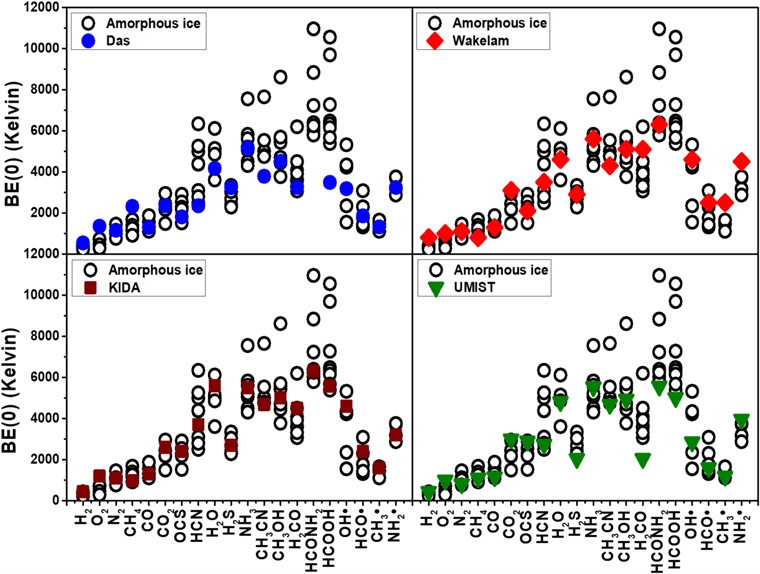
**Figure 11.** Comparison of the computed zero-point energy corrected BE(0)s for the amorphous ice model with respect to those by Das et al., by Wakelam et al., and reported in the KIDA and UMIST databases (McElroy et al. 2013; Wakelam et al. 2015, 2017; Das et al. 2018).
Download figure:
Standard image High-resolution image

4.1.3. Comparison with Values in Astrochemical Databases

Two databases list the BEs of the species used by the astrochemical models: the Kinetic Database for Astrochemistry (KIDA, http://kida.astrophy.u-bordeaux.fr/; Wakelam et al. 2015) and UMIST (http://udfa.ajmarkwick.net/index.php; McElroy et al. 2013). The comparison between our newly computed values and those reported in the two databases is shown in Figure 11. The general remarks that we wrote for the comparison with the literature experimental and theoretical values (Sections 4.1.1 and 4.1.2) roughly apply here: the databases quote BE values in the low end of ours. This is not surprising, as the databases are compiled based on the experimental and theoretical values in the literature. We just want to emphasize here, once again, that the sites with large BEs are lacking, and this may have important consequences in the astrochemical model predictions.

4.2. Astrophysical Implications

BEs enter in two hugely important ways in the chemical composition of interstellar objects/clouds: (i) they determine at what dust temperature the frozen species sublimate, and (ii) they determine at what rate the species can diffuse in the ice, as the diffusion energy is a fraction of the BE species. Both processes are mathematically expressed by an exponential containing the BE. Therefore, even relatively small variations of the BE can cause huge differences in the species abundances in the gas phase and on the grain surfaces, where they can react with other species.

In this context, probably the most important astrophysical implication of the present study is that in our ASW model (which is likely the best description to represent the interstellar amorphous ice so far available in the context of the BE estimates) a species does not have a single value, but a range of values that depend on the species itself and the site where it is bound. The range can spread by more than a factor of two: this obviously can have a huge impact on the modeling and, consequently, our understanding of the interstellar chemical evolution.

4.2.1. Impact of Multiple BEs in Astrochemical Modeling

To give a practical example of the impact on the gaseous abundance, we built a toy model for the interstellar ice and simulated the desorption rate of the ice as a function of the temperature. Our scope here is not to compare the toy model predictions with astronomical observations or laboratory experiments: we only mean to show how multiple BEs (we used the electronic BEs) would lead, in principle, to a different behavior of the ice sublimation process. Therefore, we developed a toy model that does not contain diffusion or reaction processes on the ice surface or rearrangement of the ice during the ice heating, but only a layered structure with two species, specifically water and methanol, where molecules have the range of BEs calculated in Section 3. We then show how the multiple BEs affect the temperature at which peaks of desorption appear, considering that only species at the surface of the ice, namely, exposed to the void, can sublimate (and not the entire bulk). In this toy model, we considered 10 layers for an icy grain mantle, where the bottom five are made entirely of water and each of the top five layers contains 80% water and 20% methanol. The methanol molecules with different BEs are distributed randomly on each layer, with the same proportion of BE sites. Looking at the BE values computed with the DFT//HF-3c method on the ASW model, methanol has eight BE values (4414, 5208, 5509, 6362, 6519, 6531, 6663, and 10,091 K), and at each layer there will be 12.5% methanol molecules with each of the eight BEs. The same applies for water molecules, for which we have computed five possible BEs (4222, 5689, 5845, 6014, and 7156 K), with 20% water molecules with each BE. In this model, only molecules of the layers in contact with the void can evaporate: for example, methanol molecules can be trapped if they have water molecules with larger BEs on top of them.

We start with an ice temperature of 10 K, and at the end it reaches 400 K in 10⁵ yr, to simulate the heating of a collapsing solar-like protostar. The plot of the desorption rates is shown in Figure 12, where we also show them assuming the BE values from the KIDA database for methanol and water, respectively. First, when only the KIDA values for BE are assumed, water molecules desorb at about 110 K; methanol has two peaks of desorption rates, the first at about 95 K, corresponding to the desorption of the methanol molecules not trapped by the water molecules, and the second peak at about 110 K, when all water molecules desorb so that no methanol molecules are trapped. Note that the desorption of the water molecules of the bottom layers arrives at a slightly larger temperature.

Not surprisingly, the introduction of multiple BEs produces multiple peaks of desorption, for both water and methanol. Figure 12 shows that the water desorption rate has a small peak at ∼75 K, a larger one at ∼120 K, then another at ∼140 K, and, finally, a last peak at ∼190 K. Methanol starts to desorb at 80 K, the bulk is desorbed between 120 and 140 K, and a last peak is seen around 190 K. We emphasize again that this is a toy model meant to show the potential impact of the new BEs on the astrochemical modeling. The details will depend on the real structure of the water ice and how molecules are distributed on the icy mantles. They will determine how many sites have a certain BE value and how molecules are trapped in the ice. As a very general remark, we can conclude that species can be in the gas phase at lower and higher dust temperatures than if one only considers a single BE.

4.2.2. Looking Forward: Implementation of Multiple BEs in Astrochemical Models

Our toy model introduced in the previous subsection shows the importance of considering multiple BEs for each species in the astrochemical models to have more realistic predictions. In this work, we provide the possible BEs for 21 species (Table 3). Very likely, they cover most of the possibilities, as they span a large range of H-bonds within the water molecules of the ASW. However, from a computational standpoint, such an adsorption variability has to be fully explored, in which plotting the different calculated BEs in histograms is useful to provide insights on the shape of the BE distribution (Song & Kästner 2017). Moreover, in order to build a reliable astrochemical model, one would also need to know the relative probability for each BE, and our present study is unable to provide sensible numbers. For that, a statistical study on an ASW model that is much larger than the one used here is necessary. This is a step that we indeed plan to take in future studies. Meanwhile, we adopted a distribution in which we assign an equal fraction of molecules to each BE. If one looks carefully at the distribution of the BEs for each molecule, they are not uniformly distributed but peak around some values: for example, methanol has a peak around 6000 K and an extreme value of 10,091 K only, so that, very likely, this site will be less populated than the sites around 6000 K, as shown by Figure 10. Yet, considering even a smaller fraction of these extreme values may have important consequences, for example, in the so-called snow lines of protoplanetary disks, or even on the observed abundances toward hot cores and hot corinos, or, finally, toward prestellar cores.

4.2.3. Comments on N₂, CO, and HCl

Finally, we would like to comment on three species of the studied list, N₂, CO, and hydrogen chloride (HCl).

N₂ and CO: Our computations show that the BE of CO is definitively larger than that of N₂, against the values that are in the astrochemical databases (see Table 3): on average, our computed BEs differ by about 400 K, whereas in the databases the difference is 200 and 360 K in KIDA and UMIST, respectively. This difference very likely can explain why observations detect N₂H⁺, which is formed in the gas phase from N₂, where CO is already frozen on the grain mantles (e.g., Bergin et al. 2002; Tafalla et al. 2004; Redaelli et al. 2019), a debate that has been going on for almost two decades (e.g., Öberg et al. 2009; Pagani et al. 2012). In order to quantify the effect, a specifically focused modeling will be necessary, which is beyond the scope of the present work. Here we want simply to alert that the new BEs might explain some long-standing mysteries. Another comment regards the difference in the BEs on crystalline surfaces and ASW. Again, the CO BE is about 500 K larger than that of N₂, and both are larger by about 300 K than those on the ASW, a difference that also has an impact on the snow lines of these two species in protoplanetary disks, where crystalline water ices have been detected (Terada & Tokunaga 2012).

HCl: Astrochemical models predict that HCl is the reservoir of Cl in molecular gas (e.g., Schilke et al. 1995; Neufeld & Wolfire 2009; Acharyya & Herbst 2017). However, all the observations carried out so far have found that only a tiny fraction of Cl is in the gaseous HCl, even in sources where all the grain mantles are supposed to be completely sublimated (Peng et al. 2010; Codella et al. 2011; Kama et al. 2015). One possible explanation is that HCl, once formed in the gas phase, is adsorbed on the grain icy mantles and dissociates, as shown by our calculations on the ASW model and also by previous calculations on the crystalline P-ice model (Casassa 2000) and for more sophisticated proton-disordered crystalline ice models (Svanberg et al. 2000). It is a matter to be studied whether the sublimation of the water, when the dust reaches about 100–120 K, would also provide a reactive channel transforming the Cl anion in the neutral atom, the latter obviously unobservable. This would help in solving the mystery of HCl not being observed in gas phase. Furthermore, if that were the case, the population of the chemically reactive atomic Cl would be increased, with an important role in the gas-phase chemistry (see, e.g., Balucani et al. 2015; Skouteris et al. 2018).

5. Conclusions

In this work, we present both a new computational approach and realistic models for crystalline and amorphous water ice to be used to address an important topic in astrochemistry: the BEs of molecules on interstellar ice surfaces. We simulated such surfaces by means of two (antipodal) models, in both cases adopting a periodic approach: a crystalline and an amorphous 2D slab model. We relied on DFT calculations, using the B3LYP-D3 and M06-2X widely used functionals. This approach was further validated by an ONIOM-like correction at the CCSD(T) level. Results from this combined procedure confirm the validity of the BEs computed with the adopted DFT functionals. The reliability of a cost-effective HF-3c method adopted to optimize the structures at the amorphous ice surface sites was proved by comparing the BEs computed at the crystalline ice surface at the DFT//DFT and DFT//HF-3c levels, which were found to be in very good agreement.

On both ice surface models, we simulated the structure and adsorption energetic features of 21 molecules, including 4 radicals, representative of the most abundant species of the dense ISM. A main conclusion is that the crystalline surfaces only show very limited variability in the adsorption sites, whereas the amorphous surfaces provide a wide variety of adsorption binding sites, resulting in a distribution of the computed BE. Furthermore, BE values at crystalline ice surface are in general higher than those computed at the amorphous ice surfaces. This is largely due to the smaller geometry relaxation cost upon adsorption compared to the amorphous cases, imposed by the tighter network of interactions of the denser crystalline ice over the amorphous ice.

Finally, the BEs obtained by the present computations were compared with literature data, from both experimental and computational works, as well as those on the public astrochemical databases KIDA and UMIST. In general, our BEs agree relatively well with those measured in the laboratory, with the exception of O₂ and, to a lesser extent, H₂. On the contrary, previous computations of BEs, which considered a very small number of (≤6) water molecules, provide generally lower values with respect to our new computations and, with no surprise, miss the fact that BEs have a spread of values that depend on the position of the molecule on the ice. Since the two astrochemical databases mentioned above are based on the literature data, our BEs differ, sometimes substantially, from those quoted and do not report multiple BE values.

We discussed some astrophysical implications, showing that the multiple computed BEs give rise to a complex process of interstellar iced mantle desorption, with multiple peaks as a function of the temperature that depends (also) on the ice structure. Our new computations do not allow us to estimate how the BEs are distributed for each molecule, as only a statistical study is necessary for that. The new (multiple) BEs of N₂ and CO might explain why N₂H⁺ depletes later than CO in prestellar cores, while the relatively low abundance of HCl, observed in protostellar sources, could be due to the fact that it dissociates into the water ice, as shown by our calculations.

Finally, the present study shows the importance of theoretical calculations of BEs on as realistic as possible ice surfaces. This first study of 21 molecules needs to be extended to the hundreds of molecules that are included in the astrochemical models to have a better understanding of the astrochemical evolution of the ISM.

A part of the computational results were from the SF Master thesis "Ab initio quantum mechanical study of the interaction of astrochemical relevant molecules with interstellar ice models," Dipartimento di Chimica, University of Torino, Torino, 2018. S.F., L.Z., and P.U. acknowledge financial support from the Italian MIUR (Ministero dell'Istruzione, dell'Università e della Ricerca) and from Scuola Normale Superiore (project PRIN 2015, STARS in the CAOS—Simulation Tools for Astrochemical Reactivity and Spectroscopy in the Cyberinfrastructure for Astrochemical Organic Species, cod. 2015F59J3R). The Italian CINECA consortium is also acknowledged for the provision of supercomputing time for part of this project. A.R. is indebted to the "Ramón y Cajal" program. MINECO (project CTQ2017-89132-P) and DIUE (project 2017SGR1323) are acknowledged. This project has received funding from the European Union's Horizon 2020 research and innovation program under the Marie Sklodowska-Curie grant agreement No. 811312 for the project "Astro-Chemical Origins" (ACO) and from the European Research Council (ERC) under the European Union's Horizon 2020 research and innovation program, for the Project "The Dawn of Organic Chemistry" (DOC), grant agreement No. 741002. Finally, we wish to acknowledge the extremely useful discussions with Prof. Gretobape.

Appendix A: Computational Details

In CRYSTAL17, the multielectron wave function is built as a Slater determinant of crystalline/molecular orbitals, which are linear combinations of localized functions on the different atoms of the structure that are called atomic orbitals (AOs). In a similar manner, the AOs are constructed by linear combinations of localized Gaussian functions that form a basis set. The basis set employed for this work is an Ahlrichts-TVZ (Schäfer et al. 1992), added with polarization functions.

A.1. BEs, Counterpoise, and Zero-point Energy Corrections

In a periodic treatment of surface adsorption phenomena one of the most relevant energy values, useful to describe the interacting system, is the BE, which is related to the interaction energy ΔE, so that

$\begin{eqnarray}&&\mathrm{BE}=-{\rm{\Delta }}E.\end{eqnarray} \tag{ A1 }$

The BE per unit cell per adsorbate molecule BE is a positive quantity (for a bounded adsorbate) defined as

$\begin{eqnarray}&&\mathrm{BE}=[{E}_{m}(M//M)+E(S//S)]-E({SM}//{SM}),\end{eqnarray} \tag{ A2 }$

where E(SM//SM) is the energy of a fully relaxed unitary cell containing the surface slab S in interaction with the adsorbate molecules M, E(S//S) is the energy of a fully relaxed unitary cell containing the slab alone, and E_m(M//M) is the molecular energy of the free fully optimized adsorbate molecule (the symbol following the double slash identifies the geometry at which the energy, E, is calculated)

$\begin{eqnarray}&&\mathrm{BE}={\mathrm{BE}}^{* }-\delta {E}_{S}-\delta {E}_{M}\end{eqnarray} \tag{ A3 }$

$\begin{eqnarray}&&\delta {E}_{S}=E(S//{SM})-E(S//S)\end{eqnarray} \tag{ A4 }$

$\begin{eqnarray}&&\delta {E}_{M}=E(M//{SM})-{E}_{m}(M//M)\end{eqnarray} \tag{ A5 }$

$\begin{eqnarray}&&{\mathrm{BE}}^{* }=[E(S//{SM})+E(M//{SM})]-E({SM}//{SM}),\end{eqnarray} \tag{ A6 }$

in which δE_S is the deformation energy of the surface (δE_S > 0), whereas δE_M (= ΔE_M + ΔE_L) counts both the deformation energy of the molecule (ΔE_M) and the lateral intermolecular interactions (ΔE_L) between the infinite molecule images in the same spatial configuration occurring in the SM periodic system. The pure molecule's deformation energy can be computed as

$\begin{eqnarray}&&{\rm{\Delta }}{E}_{M}={E}_{m}(M//{SM})-{E}_{m}(M//M),\end{eqnarray} \tag{ A7 }$

in which E_m(M//SM) is the molecular energy of the molecule frozen at the geometry occurring on the surface and E_m(M//M) is the molecular energy of a fully optimized free molecule, so that ΔE_M > 0. The lateral intermolecular interactions, ΔE_L, are defined as

$\begin{eqnarray}&&{\rm{\Delta }}{E}_{L}=E(M//{SM})-{E}_{m}(M//{SM})\end{eqnarray} \tag{ A8 }$

and can be either positive (repulsion) or negative (attraction). With those positions, the BE* interaction energy is then deformation and lateral interaction free, being the result of energy differences between periodic calculations carried out at the geometry of the SM system. For instance, E(M//SM) is the energy of the unit cell of a crystal containing only a molecule in the same geometry assumed in the SM system. The above BE definition can be easily recast to include the BSSE correction, using the same counterpoise method adopted for intermolecular complexes (Boys & Bernardi 1970; Davidson & Feller 1986). The definition of the BSSE-corrected interaction energy BE^C is then

$\begin{eqnarray}&&{\mathrm{BE}}^{C}={\mathrm{BE}}^{* C}-\delta {E}_{S}-{\rm{\Delta }}{E}_{M}-{\rm{\Delta }}{E}_{L}^{C}\end{eqnarray} \tag{ A9 }$

$\begin{eqnarray}\begin{array}{rcl}{\mathrm{BE}}^{* C} & = & [E(S[M]//{SM})+E([S]M//{SM})]\\ & & -\ E({SM}//{SM})\end{array}\end{eqnarray} \tag{ A10 }$

$\begin{eqnarray}&&\mathrm{BSSE}=\mathrm{BE}-{\mathrm{BE}}^{C},\end{eqnarray} \tag{ A11 }$

in which E(S[M]//SM) and E([S]M//SM) are the energy of the slab plus the ghost functions of the molecules and the energy of the infinite replica of molecules with the ghost functions of the underneath slab, respectively. Because the variational theorem ensures that BE^*C < BE*, it immediately results that BSSE > 0.

Each of the terms of Equation (A2) can be corrected by the zero-point vibrational contribution (in the harmonic approximation), ZPE, therefore arriving at the definition of the zero-point correct BE, BE(0), as

$\begin{eqnarray}\begin{array}{rcl}\mathrm{BE}(0) & = & [{E}_{m}(M//M)+E(S//S)]-E({SM}//{SM})\\ & & +\ [\mathrm{ZPE}(M)+\mathrm{ZPE}(S)-\mathrm{ZPE}({SM})]\end{array}\end{eqnarray} \tag{ A12 }$

$\begin{eqnarray}&&\mathrm{BE}(0)=\mathrm{BE}-{\rm{\Delta }}\mathrm{ZPE}\end{eqnarray} \tag{ A13 }$

$\begin{eqnarray}&&{\rm{\Delta }}\mathrm{ZPE}=\mathrm{ZPE}({SM})-\mathrm{ZPE}(M)-\mathrm{ZPE}(S).\end{eqnarray} \tag{ A14 }$

In this work the ΔZPE has been evaluated for the crystalline ice cases only, and then the scaling factor found in the linear fit of Figure 13 was adopted to correct the BEs for the amorphous ice model for the reason described in Section 2.1.

A.2. Details on HCl Adsorbed on Crystalline and Amorphous Ices

Our calculations showed that HCl remains molecularly adsorbed at the crystalline ice surface. At the amorphous one it spontaneously deprotonates, making a locally stable ion pair (Cl⁻/H₃O⁺) (see the figure below). The reason is that for the surface selected to represent the crystalline ice, the ion pair cannot be stabilized by a large enough network of H-bonds owing to the rigidity of the structure. On the contrary, at amorphous surface, Cl⁻ is engaged in three H-bonds, while the hydronium ion remains embedded in the H-bonds provided by the ice surface. A good solvation of the ion pair is the key determining the final fate of HCl at the ice surfaces (molecular or ion pair) as already pointed out many years ago by Novoa and Sosa for a small water cluster hosting HCl (Novoa & Sosa 1995). While deprotonation of HCl cannot be excluded for specific crystalline ice surface sites as simulated by Svanberg et al. (2000) when enough dH can stabilize the anion, deprotonation would be much more common at amorphous ice surface or locally distorted crystalline ones, due to the presence of favorable local environment (see Figure 14). Dissociative adsorption was found early by Horn et al. (1992) through RAIRS spectroscopy of DCl adsorption on thin D₂O film, and by Olanrewaju et al. (2011) through thermal and electron-stimulated desorption experiments.

**Figure 14.** Enlarged views of HCl adsorbed on a crystalline and amorphous ice models.
Download figure:
Standard image High-resolution image

A.3. CRYSTAL17 Computational Parameters

In order to optimize the values of the shrinking factor, the tolerances on integrals of the integration grid (SHRINK, TOLINTEG, and GRID parameters in the code; Dovesi et al. 2018) as described in Section 2 of the article, NH₃ has been adopted as a test case. Geometry optimizations for the adsorption process on the crystalline slab model have been run with the previously described computational scheme, varying one by one the aforementioned parameters, with convergence on the pure ΔE as defined by Equation (A1) being the threshold. For this benchmark calculation, BSSE, distortion, and lateral interaction contributions have not been computed. Results are resumed in what follows.

From Table 4 it is clear that ΔE is practically unaffected by the SHRINK value; thus, SHRINK = (2 2) has been used for all calculations, allowing the saving of computational time.

Table 4. Optimization of the SHRINK Parameter

SHRINK	k Points in BZ	ΔE (K)
2 2	4	7873
3 3	5	7889
4 4	10	7889
5 5	13	7890
6 6	20	7890
7 7	25	7890
8 8	34	7890

Note. Tolerances of integrals (TOLINTEG) and integration grid (XLGRID) are fixed to default values.

Download table as: ASCII Typeset image

As for the SHRINK parameter, the variations of TOLINTEG values (see Table 5) do not practically affect the final ΔE value. Consequently, its values have been set equal to 7, 7, 7, 7, and 14.

Table 5. Optimization of the TOLINTEG Parameter (SHRINK = 2 2 and XLGRID)

TOLINTEG	ΔE (K)
6 6 6 6 12	7889
7 7 7 7 14	7906
8 8 8 8 16	8063
9 9 9 9 18	7981
10 10 10 10 20	7890

Download table as: ASCII Typeset image

Again, the ΔE is practically unaffected by changing the adopted grid (see Table 6); therefore, XLGRID was selected for all the remaining calculations. Resuming, every other calculation has been carried out with SHRINK = (2 2), TOLINTEG = (7 7 7 7 14), and XLGRID as computational parameters.

Table 6. Optimization of the Integration Grid Parameter (SHRINK = 2 2 and TOLINTEG = 7 7 7 7 14)

GRID	ΔE (K)
XLGRID	7951
XXLGRID	7951

Download table as: ASCII Typeset image

A.4. Description of Dispersive Forces

We optimized the geometry of two parallel benzene rings that interact with each other just because of dispersive forces given the apolar nature of the molecule. The results of Figure 15 clearly show that the B3LYP functional needs some a posteriori correction (like Grimme's D3) for dispersive forces in order to describe correctly the interaction (Grimme et al. 2010), whereas the M06-2X functional is able to describe it correctly without any a posteriori correction (Zhao & Truhlar 2008).

**Figure 15.** Initial and optimized geometry of two parallel benzene rings obtained with B3LYP (without dispersion corrections), B3LYP-D3 and M06-2X functionals. Distances between the planes of the two rings are reported in angstroms.
Download figure:
Standard image High-resolution image

A.5. ONIOM2 Correction

In Table 7 we summarize the single components (namely, BE(CCSD(T), μ-2H₂O) extrapolated, BE(DFT, μ-2H₂O), BE(DFT, ice), and finally the corrected BE(ONIOM2)) of the ONIOM2 correction done with the extrapolation procedure already described in Section 2.

Table 7. Summary of the Components Used for the Calculation of the ONIOM2 Correction to the BEs

Species	BE(CCSD(T), μ–nH₂O) Extrapolated	BE(DFT, μ–nH₂O)	BE(DFT, ice)	BE(ONIOM2)	$\|$ Diff $\|$
H₂	843	796	1192	1240	47
CO	1127	1165	2356	2318	38
CO₂	1939	1817	3442	3564	121
OCS	1354	1138	3478	3695	216
H₂S	2443	2875	5679	5248	432
HCN	3300	3453	5795	5642	153
H₂CO	3199	3114	6490	6575	85
HCl	3993	4475	6501	6019	482
NH₃	4246	4389	7376	7233	143
CH₃OH	5196	5275	8681	8602	79
HCOOH	6263	6223	9522	9562	40
HCONH₂	5080	5056	9614	9638	24
OH•	4492	4502	6542	6532	10
NH₂•	3021	2788	6043	6276	233
HCO•	2339	2088	3474	3725	251

Note. The last column shows the absolute value of the difference between the BE(DFT, μ-2H₂O) value and the corrected BE(ONIOM2).

Download table as: ASCII Typeset image

Appendix B: Crystalline Adsorption Geometries

The final optimized structures, together with BEs and structural properties for every molecule in our set, are presented in this appendix (see, e.g., Figure 16). For some notable cases, more than one initial structure has been modeled. All energetic quantities are in kelvin (K), while distances are in Å. For every molecule, the gas-phase optimized geometry and its ESP map are also presented. In the latter, the isovalue for the electron density is set equal to 1 × 10⁻⁶ au, while the values for the ESP (again in au) vary case by case and thus are reported close to the RGB scale legend.

**Figure 16.**
I) Representation of the hydrogen (H₂) molecule along with its ESP surface, BSSE-corrected binding energies (BE) with (*disp*) and without (*no disp*) dispersion. II) Top view of H₂-(010) P-ice surface interaction (unit cell highlighted in blue). III) Detail of the side view. (The complete figure set (23 images) is available.)
Download figure:
Standard image High-resolution image

Appendix C: Surface Distortion Energy on ASW

In Table 8 we present the distortion energy contributions calculated on the amorphous slab that will be compared with the same contributions calculated on the (010) P-ice model for some notable cases.

Table 8. Comparison of the Distortion Energy Contributions (in Kelvin) Calculated on the (010) P-ice Slab and the Mean Value of These Contributions Calculated on the Different Adsorption Cases on the Amorphous Ice Model

Species	δE_s Crystalline Ice	$\langle$ δE_s $\rangle$ Amorphous Ice
CH₃OH	662	2790
H₂O	565	3211
HCN	589	1299
HCOOH	878	1660
NH₃	734	1082

Download table as: ASCII Typeset image

Appendix D: Basis Set A-VTZ*

In Tables 9–14 we provide the basis sets in CRYSTAL17 format, used for H, C, N, O, S, and Cl atoms, respectively.

Table 9. Basis Set for the H Atom in CRYSTAL17 Format Used in This Work

H	0
S	3	1
		34.06134	6.03E-03
		5.123575	4.50E-02
		1.164663	0.201897
S	1
		0.32723	1
S	1
		0.103072	1
P	1
		0.8	1

Download table as: ASCII Typeset image

Table 10. Basis Set for the C Atom in CRYSTAL17 Format Used in This Work

C	0
S	5	1
		8506.038	5.34E−04
		1275.733	4.13E−03
		290.3119	2.12E−02
		82.0562	8.24E−02
		26.47964	0.240129
S	1
		9.241459	1
S	1
		3.364353	1
S	1
		0.871742	1
S	1
		0.363524	1
S	1
		0.128731	1
P	4
		34.7095	5.33E−03
		7.959088	3.59E−02
		2.378697	0.142003
		0.815401	0.342031
P	1
		0.289538	1
P	1
		0.100848	1
D	1
		1.6	1
D	1
		0.4	1

Download table as: ASCIITypeset images: 1 2

Table 11. Basis Set for the N Atom in CRYSTAL17 Format Used in This Work

N	0
S	5	1
		11913.42	−5.23E−04
		1786.721	−4.04E−03
		406.5901	−2.08E−02
		114.9253	−8.12E−02
		37.10588	−0.23871
S	1
		12.97168	1
S	1
		4.730229	1
S	1
		1.252518	1
S	1
		0.512601	1
S	1
		0.179397	1
P	4
		49.21876	5.55E−03
		11.34894	3.81E−02
		3.428509	0.149414
		1.179951	0.348982
P	1
		0.417261	1
P	1
		0.142951	1
D	1
		2	1
D	1
		0.5	1

Download table as: ASCII Typeset image

Table 12. Basis Set for the O Atom in CRYSTAL17 Format Used in This Work

O	0
S	5	1
		15902.65	5.15E−04
		2384.954	3.98E−03
		542.7196	2.05E−02
		153.4041	8.03E−02
		49.54572	0.237668
S	1
		17.33965	1
S	1
		6.330336	1
S	1
		1.699588	1
S	1
		0.689545	1
S	1
		0.23936	1
P	4
		63.27052	6.07E−03
		14.62331	4.19E−02
		4.448952	0.161569
		1.528151	0.356828
P	1
		0.529973	1
P	1
		0.175094	1
D	1
		2.4	1
D	1
		0.6	1

Download table as: ASCII Typeset image

Table 13. Basis Set for the S Atom in CRYSTAL17 Format Used in This Work

S	0
S	5
		103954	2.47E−04
		15583.79	1.92E−03
		3546.129	9.96E−03
		1002.681	4.04E−02
		324.9029	0.130675
S	1
		115.5123	1
S	2
		44.52821	0.504036
		18.39789	0.230681
S	1
		5.510068	1
S	1
		2.125987	1
S	1
		0.436919	1
S	1
		0.157309	1
P	5
		606.6937	2.32E−03
		143.507	1.86E−02
		45.74616	8.60E−02
		16.87291	0.252484
		6.63992	0.446327
P	1
		2.672714	1
P	1
		1.000009	1
P	1
		0.354389	1
P	1
		0.116713	1
D	1
		1.1	1
D	1
		0.275	1

Download table as: ASCII Typeset image

Table 14. Basis Set for the Cl Atom in CRYSTAL17 Format Used in This Work

Cl	0
S	5
		117805.8	2.42E−04
		17660.27	1.87E−03
		4018.597	9.74E−03
		1136.223	3.95E−02
		368.1206	0.127972
S	1
		130.8615	1
S	2
		50.47901	0.428741
		20.91681	0.196685
S	1
		6.353139	1
S	1
		2.494801	1
S	1
		0.543359	1
S	1
		0.194344	1
P	5
		681.0688	2.37E−03
		161.1136	1.89E−02
		51.38664	8.78E−02
		18.95851	0.257074
		3.003516	0.371524
P	1
		7.456529	1
P	1
		1.060936	1
P	1
		0.39452	1
P	1
		0.133233	1
D	1
		1.3	1
D	1
		0.325	1

Download table as: ASCII Typeset image

Binding Energies of Interstellar Molecules on Crystalline and Amorphous Models of Water Ice by Ab Initio Calculations

Article metrics

Permissions

Share this article

Author e-mails

Author affiliations

ORCID iDs

Dates

Abstract

1. Introduction

2. Computational Details

2.1. Structure of the Ice: Periodic Simulations

2.2. BE Calculation and Counterpoise Correction

2.3. BE Refinement with the Embedded Cluster Method

3. Results

3.1. Ice Surface Models

3.1.1. Crystalline Ice Model

3.1.2. Amorphous Solid Water (ASW)

3.2. BEs on Crystalline Ice

3.2.1. BE Computed with DFT//DFT Method

3.2.2. The ONIOM2 Correction and the Accuracy of the DFT//DFT BE Values

3.2.3. BE Computed with Composite DFT/HF-3c Method

3.3. BEs on Amorphous Solid Water

4. Discussion

4.1. Comparison BE Values in the Literature

4.1.1. Comparison with Experimental Values

4.1.2. Comparison with Computed Values

4.1.3. Comparison with Values in Astrochemical Databases

4.2. Astrophysical Implications

4.2.1. Impact of Multiple BEs in Astrochemical Modeling

4.2.2. Looking Forward: Implementation of Multiple BEs in Astrochemical Models

4.2.3. Comments on N2, CO, and HCl

5. Conclusions

Appendix A: Computational Details

A.1. BEs, Counterpoise, and Zero-point Energy Corrections

A.2. Details on HCl Adsorbed on Crystalline and Amorphous Ices

A.3. CRYSTAL17 Computational Parameters

A.4. Description of Dispersive Forces

A.5. ONIOM2 Correction

Appendix B: Crystalline Adsorption Geometries

Appendix C: Surface Distortion Energy on ASW

Appendix D: Basis Set A-VTZ*

4.2.3. Comments on N₂, CO, and HCl