A unified approach to model peripheral nerves across different animal species

Stretching experiments

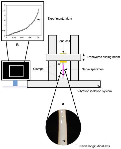
A peroneal nerve was dissected from a posterior limb of a Large White pig (∼10 months old), which was slaughtered in conformity with the Italian National Regulation and frozen until experiments. Before experiments, the nerve specimen (96 mm long with a cross-sectional area of ∼6.39 mm²) was gradually defrosted and re-hydrated for about one hour at room temperature in a bath of aqueous saline solution isotonic to the blood (0.9% sodium chloride) to minimize the time dependence of the tissue hydration. The length of the specimen between clamps was 69 mm, and its physiological characteristics were kept by regularly spraying saline moisture on its external surface in order to maintain the initial level of hydration. Stretching experiments were carried out at room temperature (∼25 ± 1 °C), by using an Instron R4464 testing machine (Instron Corporation, Canton, MA, USA) with a standard load cell (Instron load cell, cell type 2525–808, max force 10 N, accuracy 0.25% Full Scale Output; (Instron Corporation, Canton, MA, USA) as shown in Fig. 1.

More specifically, the nerve was stretched (velocity v = 10 mm/min (Bora, Richardson & Black, 1980); maximum strain 8%) after preconditioning to minimize viscoelastic effects (Fung, 1993). The axial force was digitally recorded for five extensions of the nerve.

Theoretical connection between stress and stretch

The peripheral nervous tissue (PNT) was modelled as a homogeneous and incompressible material and, according to previous literature (Alexander, Barkmeier-Kraemer & Vande Geest, 2010), its mechanical behavior was described through an invariant based strain energy function. More specifically, here, a polynomial hyperelastic strain energy function in Yeoh form (Yeoh, 1993) was proposed: (1)${\displaystyle \Psi \left(I_1\right)=c_1\left(I_1-3\right)+c_2{\left(I_1-3\right)}^2+c_3{\left(I_1-3\right)}^3}$ where c₁, c₂, c₃ ∈ ℜ were scalar coefficients. The Cauchy stress tensor was expressed in function of both the first strain invariant (I₁) and the deformation gradient F as: (2)${\displaystyle \sigma =-k\mathbf{I}+2\frac{\partial \Psi \left(I_1\right)}{\partial I_1}{\mathbf{FF}}^{\mathbf{T}}}$ where k was an indeterminate Lagrange multiplier, accounting for boundary conditions, while I and F^T were, respectively, the unit tensor and the transposed of the deformation gradient. Since I₁ = tr(FF^T), and F were expressed as a function of principal stretches, Eq. (2) provided a theoretical connection between stress and stretch. A homogeneous, triaxial stretch state was assumed, thus the deformation gradient and the first strain invariant were written in function of the longitudinal stretch λ. Considering both incompressibility constraint and experimental boundary conditions (through which k in Eq. (2) was determined), the theoretical transverse stretch was $1∕\sqrt{\lambda }$, while the longitudinal component of the Cauchy stress was expressed as: (3)${\displaystyle {\sigma }_z=\frac{{\wp }^{\left[9\right]}\left(\lambda ,c_1,c_2,c_3\right)}{{\lambda }^3}}$ where ℘^[9](λ, c₁, c₂, c₃) = 3c₃λ⁹ + (2c₂ − 18c₃)λ⁷ + 9c₃λ⁶ + (27c₃ − 6c₂ + c₁)λ⁵ + (2c₂ − 18c₃)λ⁴ + (−27c₃ + 6c₂ − c₁)λ² + (36c₃ − 4c₂)λ − 12c₃.

Experimental data were collected for five consecutive extensions and their mean values were reported as a function of stretch and used to represent the behaviour of the specimen. Equation (3) was used to reproduce experimental data through a non-linear optimization procedure (quasi-Newton algorithm, Scilab, 2015; Scilab Enterprises S.A.S, Versailles, France), allowing the R² function to be maximized for each extension. More specifically, guess values for [c₁, c₂] were chosen (i.e., [10.00, 0]; [12.99, 0]; [0, 12.40]; [0, 11.99]; [10.00, 0]), while [c₃], was allowed to vary in the range 6,000–9,000 KPa. To explore the sensitiveness of final vales of c₁ and c₂ to changes of c₃, the difference c₁(c₃) − c₂(c₃) was plotted (for a constant R² ≃ 0.99), as shown in Fig. S1. In addition, the influence of c₃ over R² was studied for constant values of c₁, c₂, as shown in Fig. S2. Furthermore, the correlation between c₁ and c₂ values was analyzed to test their eventual independency as well as the correlation between these values and the c₃ constant.

Finally, the sensitiveness of the stress function with respect to c₁, c₂, c₃ was expressed as: SI(c_i) = (σ_maxci − σ_minci)∕σ_maxci (Hamby, 1995; Pannell, 1997), where i = 1, 2, 3, σ_maxci and σ_minci were respectively the maximum and the minimum values of stress for the maximum and minimum values of c_i, when the other constant had optimal values.

In silico model of porcine PNT

In silico models were implemented to reproduce the in vitro stretching of peripheral nerves. To provide a suitable approximation of the complex shape of the real specimen, two different lateral views were digitally acquired (Fig. S3) and numerically reproduced through ImageJ (Rasband, 1997–2017) together with the mean straight lines for each profile (see Figs. S3A, S3B). The resulting elliptical cylinder (eccentricity 0.77, major axis 3.57 mm and minor axis 2.28 mm) was, then, modelled within a FE software (Ansys ©  Academic; Ansys, Inc., Canonsburg, PA, USA) as an incompressible solid. In particular, the nerve volume was meshed (5,004 nodes and 3,450 elements (Fig. S3)) with solid elements (SOLID185), which were able to model fully incompressible hyperelastic materials with enhanced strain and mixed displacement-pressure formulation (Cescotto & Fonder, 1979; Brink & Stein, 1996). The lower side of the cylinder was fully constrained to account for the lower clamped extremity, while experimental stretches were reproduced increasing the axial displacement of the upper section (further prevented from lateral contractions). Different approaches were also investigated to minimize the time needed to calculate the stress field for the three-dimensional elliptical cylinder. First, exploiting symmetries, only a quarter of the whole volume was meshed (1,330 nodes and 828 elements (Fig. S4A)) with solid elements (SOLID185), while symmetry constraints were imposed to the lateral areas. Then, the mean elliptic cylinder (reproducing the mean surface of the nerve and having a low eccentricity), was rescaled into a circular cylinder, keeping constant the cross sectional area through the additional constraint r² = ab (where r was the radius of the new circular section, while a, b were the semi-major and semi-minor length of the elliptic section). The axial symmetry of the circular cylinder was furthermore used to study only a rectangular slice (Fig. S4B), which was eshed (210 nodes and 138 elements) with axisymmetric plane elements (PLANE182). These elements were able to model fully incompressible hyperelastic materials using enhanced strain and mixed displacement pressure formulation. Also in this case, to reproduce experimental boundary conditions, the lower line belonging to the rectangular area was fully constrained, while increasing longitudinal displacements were imposed to the upper extremity, which was prevented from radial contractions. The times needed to solve three-dimensional and bidimensional approximations were compared and differences in stress fields and lateral strains were investigated.

In silico models of cerebro-abdominal connective of Aplysia

An in silico model of the right connective of Aplysia kurodai, interconnected to the abdominal pleural ganglion, was implemented to test the suitability of the previous procedure in case of different neural structures and for very large stretches. More specifically, the cross section of the cerebro-abdominal connective was reproduced from literature images (Koike, 1987) and approximated with an ellipse (eccentricity 0.64) with semi-major and semi-minor axes respectively of 0.57 mm and 0.44 mm. Similarly, the length of the connective was taken from experimental images (i.e., 50 mm).

The solid model of Aplysia connective (Fig. S5A) was meshed with solid elements (SOLID285), which were able to model fully incompressible hyperelastic materials with mixed displacement-pressure formulation. This procedure resulted in 2,086 nodes and 7,192 elements. In this model, the upper side was fully constrained (to account for the experimental clamped extremity), while the stretch was modelled through increasing axial displacements of the lower side, which was prevented from lateral contraction at the level of the middle sphere approximating the ganglion (Fig. S5). Also in this case, the eccentricity of the connective was low, thus the cross sectional area was re-scaled into a circular one with the same size. The resulting axisymmetric circular cylinder was then reduced to a bidimensional slice (Fig. S5B), which was meshed (460 nodes and 173 elements) with plane elements (PLANE183). Indeed, these elements were able to model fully incompressible hyperelastic materials, implementing axial symmetry and large strains with mixed displacement-pressure formulation. Again, the upper side was fully constrained, while the lower one was axially displaced and prevented from radial compressions. The global computatioanl times needed to solve three-dimensional and bidimensional approximations were compared and differences in stress fields and lateral strains were investigated.

A single strain energy function to reproduce the nerve behavior across different animal species

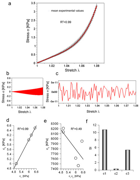
Experimental data were collected for five consecutive extensions and their mean values were reported as a function of stretch in Fig. 2A (circles). For each value, the variation range was also plotted as vertical lines (i.e., difference between minimum and maximum values).

Equation (3) was able to reproduce experimental data (R² ≃ 0.998) with c₁ = 5.89 KPa, c₂ = 5.89 KPa and c₃ = 7.75 MPa, while both the range of variation of experimental values and the errors between the mean values and the fitting curve were calculated (Figs. 2B and 2C). To further investigate the ability of Eq. (3) in reproducing each single extension, all curves were analysed. In all cases, c₁ and c₂ were almost equal (i.e., error less than 2.422⋅10⁻⁵ KPa), and had the following values 4.99 KPa , 6.49 KPa, 6.20 KPa, 5.99 KPa, 4.99 KPa, while the c₃ parameter resulted in 8.13 MPa, 7.95 MPa, 7.46 MPa, 7.61 MPa, 8.21 MPa. These values were inserted in Eq. (3), which was, then, able to fit experimental data for each curve (respectively with R² of 0.995, 0.995, 0.996, 0.996, 0.995). To test possible further cross correlations among numerical constants in Eq. (3), the c₁ values were plotted versus the corresponding value of c₂ for each extension, while the values of c₃ were also plotted versus c₁, c₂. This procedure showed a positive and very strong correlation in the first case (i.e., R² > 0.99, as expected), while a weak correlation in the second one R² = 0.49, as shown in Figs. 2D and 2E. Finally, the sensitivity index (SI) for c₁, c₂, c₃ constants resulted respectively in 10.79, 0.32, 5.38 (Fig. 2F).

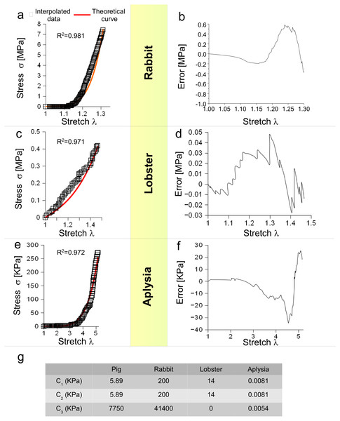
Moreover, Eq. (3) was tested for different animal species (vertebrates and invertebrates) and for different levels of stretch. More specifically, the behaviour of a rabbit nerve until λ ≃ 1.3 was reproduced (R² = 0.981) for c₁, c₂ = 0.2 MPa and c₃ = 43.7 MPa, with errors (between data and theoretical curve) ranging from −0.38 to +0.58 MPa (Figs. 3A and 3B). Similarly, the stress/stretch curve of lobster nerve was approximated (R² = 0.971) for λ = 1.5 with c₁, c₂ = 0.14 MPa and c₃ = 0, with errors in the range −0.03,  + 0.05 MPa (Figs. 3C and 3D). Finally, the stress/stretch curve of a cerebro-abdominal connective of Aplysia (λ = 5) was reproduced (R² = 0.972 for c₁, c₂ = 0.0081 KPa and c₃ = 0.0054 KPa), with errors ranging between −34.41 and +25.31 KPa (Figs. 3E and 3F). A comparison between coefficients was also performed and shown in Table of Fig. 3G.

In silico models of PNT

Three-dimensional model

In Fig. 4A, the spatial distribution of displacements is shown along the X, Y, Z axes, while in Fig. 4B both the stress and strain fields are shown for the maximum stretch. Theoretical and the computational curves were compared (Fig. 4C), and their difference (within the −0.4%) was plotted as a function of stretch (Fig. 4D). Similarly, theoretical and computational strains along radial directions (X, Y axes) were compared (Fig. 4E), and their difference (within 0.0003) was plotted as a function of stretch, as shown in Fig. 4F.

Furthermore, the stress/stretch curves resulting from three-dimensional models (elliptic and re-scaled circular cylinders) (Fig. S6A) were compared, and their difference (Fig.  S6B) was within the 0.02%. Similarly, the strain along the radial direction was compared for both approximations (Fig. S6C), showing a maximum difference within −1.92⋅10⁻⁶ (Fig. S6D). In addition, the distribution of nodal stresses (for the maximum stretch) was compared showing a similar evolution (Fig. S6E) for both approximations as well as similar quantile–quantile plots (uniform distribution). Finally, nodal stresses, deriving from the elliptic cylinder, were plotted versus those coming from the circular approximation (Fig.  S6F). In this case, numerical values were grouped along a straight line and clustered around the value of 3.34 KPa.

Bidimensional model of in vitro porcine nerve

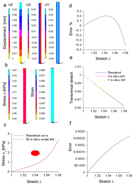
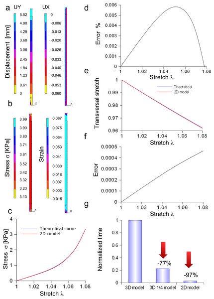
A rectangular slice coming from the axisymmetric re-scaled circular cylinder was used to approximate the nerve specimen (Fig. 5). More specifically, the displacements of the plane section along the X, Y, Z axes as well as the longitudinal stress and strain fields were computed for the maximum stretch (Figs. 5A and 5B). Theoretical and computational stress/stretch curves were compared in Fig. 5C, showing a percentage error within 0.006% (Fig. 5D). Similarly, the comparison between transversal stretches was performed (Fig. 5E), and the error resulted in 0.0005 (Fig. 5F). Finally, the time needed to compute the stress/strain fields was calculated for both the reduced models (i.e., 1∕4 of whole structure and plane axisymmetric slice), and normalized with respect to the total time needed to solve the whole elliptical cylinder. Figure 5G shows that the three-dimensional approximation (1∕4 of the structure) was able to reduce the total normalized time from 1 to 0.225, while the bidimensional one (plane slice) was able to further decrease the normalized time up to 0.029.

Three-dimensional model of the Aplysia connective

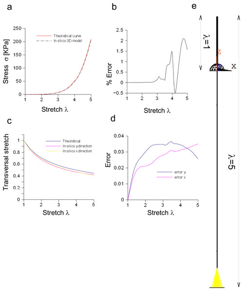
The performances of the three-dimensional in silico model of the Aplysia connective were studied and compared to theoretical results coming from the application of Eq. (3). Both theoretical and computational curves were superimposed (up to λ = 5, Fig. 6A), while the percentage difference was between −0.5% and 2.2% (Fig. 6B). Similarly, the transversal stretch deriving from the three-dimensional in silico approximation was compared to the theoretical ones (for both X and Y axes, Fig. 6C), resulting in differences within 0.039 (Fig.  6D). The deformation of the connective structure is shown in Fig. 6E, where the initial configuration (λ = 1) is plotted (upper part, wireframe) together with the final one (λ = 5) (lower part).

Bidimensional model of the Aplysia connective

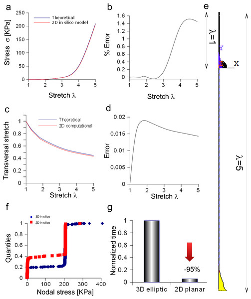
The bidimensional approximation of the Aplysia connective was able to reproduce the theoretical stress/stretch curve (up to λ = 5, Fig. 7A), showing that the percentage error remained within the 1.6% (see also some numerical oscillations in Fig. 7B). The evolution of the theoretical and computational transversal stretches was, then, studied and the resulting two curves were very close along the whole stretch range (Fig. 7C). In particular, the difference between them (within 0.019), was an increasing function up to λ = 2, while a slightly decreasing one up to λ = 5 (Fig. 7D). The deformation of the connective structure is shown in Fig. 7E, where the initial configuration (λ = 1) is plotted (upper part, wireframe), together with the final one (λ = 5, lower part). Furthermore, the quantile–quantile plot (uniform distribution) for both three-dimensional and bidimensional models of Aplysia connective were provided and compared in Fig. 7F. Although their shape was not totally superimposed, most of values were clustered at 206.7 KPa for both the approximations. Finally, the time needed to solve both three-dimensional and bidimensional models was normalized with respect to the computational time needed to solve the whole three-dimensional structure (Fig. 7G), showing that the use of the axisymmetric slice reduced this time from 1 to 0.056.

A single strain energy function across different species

In this work, a unified approach was proposed to reproduce the stress/stretch behaviour of neural structures across different animal species (vertebrate/invertebrate) through a classic formulation involving a strain energy function. The chosen function was in Yeoh-like form (Yeoh, 1993), since this formulation was suitable for a wide range of stretches, avoiding numerical instabilities due to a high number of constants (Busfield & Muhr, 2003) and overcoming stretch limitations due to other invariant-based implementations (e.g., Mooney, 1940; Rivlin, 1948). Moreover, it was able to satisfy the Drucker stability criterion (Drucker, 1957; Bergstrom, 2015) (i.e., the resulting stress always increased for increasing strains), allowing boundary value problems to be treated without further numerical complications (e.g., multiple solutions or stress oscillations due to instability). The ability of Eq. (3) in reproducing different responses was due to a certain flexibility, resulting from the interplay between numerical constants. In particular, the values of constants c₁ and c₂ were almost equal for each extension, as well as for different values of the c₃ coefficient. Indeed, a maximum error of 2.422⋅10⁻⁵ KPa (i.e., 4⋅10⁻⁴%) was found for all extensions (Fig. S1). Similarly, this difference was 3⋅10⁻³ MPa (i.e., 1.70%) for rabbit, 1.9⋅10⁻² KPa (i.e., 1.42%) for lobster, and 1⋅10⁻⁷ KPa (i.e., 1⋅10⁻³%) for Aplysia. As a consequence, c₁ and c₂ were assumed to be equal in these animal models. However, the sensitivity of the stress function to c₂ (SI = 0.38) was smaller than the sensitivity to c₁ and c₃ (respectively SI = 10.79 and SI = 5.38). In other words, both c₁ and c₃ seemed to mainly affect the behaviour of the stress function, which was able to reproduce the elastic response of several tissues, ranging from Aplysia connective to pig nerves.

Further cross connections between c₁, c₂ and c₃ were investigated (Fig. 2E), but no evidence of a correlation was found (i.e., R² = 0.49 and scattered values). Therefore, no important mutual stiffening effects (e.g., due to dehydration) were found during experiments. This was in agreement with the hypothesis of mutual independence between these two constants. As a consequence, Eq. (3) was able to reproduce in a very close way (R² > 0.99) experimental data for the large white pig model (both the mean curve and each extension) and for other animal species. However, the percentage errors was around 8–10%, since numerical oscillations arose between theoretical curve and interpolated data.

In silico models of nerves and Aplysia connective

The in silico elliptic cylinder, reproducing the mean surface of the nervous specimen, was able to closely replicate the theoretical behaviour for longitudinal and transversal stretches. Indeed, the percentage error with respect to the theoretical predictions ranged between 0.2% and −0.4% for the axial stretch (Fig. 4D), while the difference between theory and computational results was less than 0.0003 for transversal stretch (Fig. 4F). Moreover, symmetries were used to decrease the computational time needed to find the stress field of this three-dimensional structure. More specifically, both symmetry planes XZ and YZ, were used to reduce the structure to a quarter of the whole solid. Further reductions (e.g., to 1/8 of the structure) were able to reproduce the stress field (far from extreme sections), while the displacement field was different, since boundary conditions were not symmetric with respect to the XY plane. However, just the reduction of the whole structure to a quarter was able to considerably lower the computational time (−77%), as shown in Fig. 5G. A further decrease was achieved through the substitution of the initial elliptic cylinder with a circular one, which was obtained through a re-scaling procedure. Since this cylinder was axisymmetric, the dimensionality of the problem was reduced from three to two dimensions. This approach was based on the equivalence of the two solids, since the eccentricity of the initial cylinder was quite low (0.77). Indeed, not only longitudinal and transversal stretches were almost the same (respectively with percentage errors less than 0.02% for the axial one, and with difference ranging from 0 to −2⋅10⁻⁶ for the transversal one), but also the nodal stress had the same distribution and the same values, clustered around the theoretical value (Figs. S5E and Figs. S5F). The use of a bidimensional slice instead of the full structure led to computational time decrease of about 97% (Fig. S5G), while it was equivalent for the calculation of both axial and transversal stretches (i.e., percentage errors less than 0.006% and difference less than 0.0005 respectively for axial and transversal directions) (Figs. 5C–5F). The main cause of this decrease of time was the big reduction of nodes and elements, respectively from 5,004 to 210 and from 3,450 to 138, which resulted in the smaller dimension of matrices needed to solve the structure.

Equation (3) was also suitable to model the connective of Aplysia. Again, a rescaling procedure and the axial symmetry were used to lower the geometric dimension of the problem together with the time needed to achieve the solution (−95%). The bidimensional approximation provided results similar to those coming from the three-dimensional model. In particular, the percentage error was less than 1.6% and the difference lower than 0.02, respectively for axial and radial stretches. Finally, nodal stresses had a similar distribution in both cases, as shown in Figs. 6 and 7.

From nerve to bundle mechanics: towards a possible application to the regeneration of nerves

Literature studies on neural-like (Ciofani et al., 2011; Sergi et al., 2013; Sergi, Marino & Ciofani, 2015) or neural cells (Roccasalvo, Micera & Sergi, 2015) investigated the behaviour of single cells in topographical and chemical active environments (Sergi & Cavalcanti-Adam, 2017). Nevertheless, this approach could be effective to study the regeneration of peripheral nerves during the first phases, when axons grow separately. However, when they are grouped into nervous bundles, which are also formed by connective tissues, their global mechanical properties change. Thus, as the mechanical properties of a tissue (which is formed by several thousands of cells) can be mathematically handed using the ”continuum approximation”, in the same way the mechanical behaviour of a nervous bundle can be accounted for through a suitable SEF. The use of Eq. (3) to model peripheral nerves (e.g., pig and rabbit nerves) and the connective of Aplysia was not foreseen, since these structures were dissimilar and belonged to different animal species. Indeed, the cerebro-connective was formed by several axons surrounded by a transparent perineurium, so this structure was similar to a nervous bundle of big animal or human nerves (Sunderland & Bradley, 1952). Therefore, the ability of Eq. (3) in reproducing the behaviour of the connective (Koike, 1987) showed that this formulation may be also extended to model the mechanical behaviour of nervous bundles.

The functional tolerance of nerves to stretch is related to the nerve site

The shape of the stress/stretch curve varied across different species, (e.g., lobster and Aplysia curves). Equation (3) was able to account for this variability through the interplay between constants. Nevertheless, the only knowledge of these data was not able to univocally reproduce the response of the material, since this response was related both to the stiffness and to the range of extensibility of nerves (before rupture), which, in its turn, was related to the material toughness. All these characteristics could be resumed as a “functional tolerance” to stretch. Intriguingly, this functional tolerance of nerves to stretch was related to the likelihood of changes in their in situ length (Koike, 1987). As a consequence, the rabbit nerves were more extensible than the pig ones, since the rabbit body is, in general, more suitable for running and jumping than the pig body. Similarly, the high (and quite unexpected) resistance of the lobster nerve to extension was related to its very small likelihood of in situ extensions, as well as the extreme tolerance to stretch of Aplysia connective was related to the high extensibility of its body (Koike, 1987). This hypothesis seems to be supported also by the discovery of the very high stretch tolerance of ventral grooved blubber and tongue nerves in rorqual whales (Balaenopteridae) (Vogl et al., 2015). Indeed, these nerves were able to be easily extended respectively of 75% and 115% before becoming stiff. This very high tolerance to stretch was related to the large deformations of both tongue and ventral grooved blubber needed to implement an efficient feeding. Indeed, other kinds of whale nerves (i.e., intercostal and phrenic nerves) were only able to be normally stretched (12% and 18%) (Vogl et al., 2015). These findings also support the importance of the body location (and the resulting in situ stretches) to understand the mechanical response of nerves, since just in a single animal species (rorqual whales) they had a big difference in functional tolerance to stretch.