How is the atmosphere modeled? What are the energy flows, the circulation, and the behavior of water as it freezes and evaporates? Different types of atmosphere models are described. The atmosphere is important for connecting the different parts or components of the earth system. Two of these connections are related to greenhouse gases: the water (or hydrologic) cycle, and the carbon cycle. The similarities and differences between models used to simulate climate and those used to simulate weather are discussed. Details about the challenges involved in simulating the future are presented. As an example, atmospheric models are applied to studying tropical cyclones (hurricanes).
The atmosphere is critical for understanding energy flows in the climate system. The main energy input for the climate system is the sun, and the atmosphere has an important role in how solar energy enters the earth system, and how energy leaves the earth system. As we have discussed, solar energy in visible wavelengths (shortwave radiation) mostly passes through the atmosphere and is absorbed by dark surfaces, but reflected by light surfaces, including clouds. Thus, clouds are critical for the net energy input. Energy radiated from the earth in the infrared (longwave radiation) passes through the atmosphere on its way out to space. It can be absorbed not just by clouds, but also by greenhouse gases, such as water vapor (H2O) and carbon dioxide (CO2). Thus, the composition of the atmosphere is critical for understanding climate.
The atmosphere is also important for connecting the different parts of the earth system. Two of these connections are related to greenhouse gases: the water (or hydrologic) cycle, and the carbon cycle. Important parts of these cycles happen in the atmosphere. The carbon cycle is critical for understanding not just CO2 in the atmosphere, but also how carbon moves through the land surface (to be discussed in Chap. 7). The water cycle is critical for human societies and ecosystems as well as the climate system: We experience the water cycle at the surface through clouds and especially through precipitation where water hits the land surface. But water also moves energy through the earth system, and this is an important part of simulating the atmosphere. For these reasons, we start a detailed discussion of each component of the climate system with the atmosphere.
Anzeige
This chapter explores in more detail how the atmosphere is modeled in the climate system. We start with the different pieces of an atmosphere model: the energy flows, the circulation, and the transformation of water. This chapter contains a description of the types of atmosphere models. We also discuss the similarities and differences between models used to simulate climate and those used to simulate weather. Finally, we go into detail about some of the challenges involved in simulating the future evolution of the atmosphere.
5.1 Role of the Atmosphere in Climate
The atmosphere is a familiar part of our daily life, and the role of the atmosphere in climate features many aspects of weather that we observe every day.1 Figure 5.1 illustrates a schematic of the atmosphere, highlighting some of the key aspects of the atmosphere in the climate system. This figure is related to the hydrologic cycle (Fig. 2.3) and the energy budget (Fig. 5.2, reprinted from Fig. 2.2). Most notably, the atmosphere is where the energy input from the sun is distributed in the climate system. It features clouds and precipitation, and with evaporation from the land surface, this represents the atmospheric hydrologic cycle. The entire atmosphere is in motion with winds that are part of a large-scale atmospheric circulation. Vertical motion is driven by buoyancy: the difference in density of air. Warm air is less dense than cold air, so it rises. As air rises, it expands and cools. But if it cools enough, water vapor condenses and forms a cloud. This releases heat, and then the air may continue to rise: This process gives rise to clouds, and to deep vertical motions in the atmosphere.
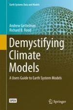
Fig. 5.1
The Atmosphere in the Climate System. Emissions and evaporation from the surface (as well as radiation) force the atmosphere from below. The sun forces the atmosphere from above. Chemistry, clouds, and wind occur in the atmosphere, along with the flows of radiation
Fig. 5.2
Energy Budget. Solar energy, or shortwave radiation (yellow) comes in from the sun. Energy is then reflected by the surface or clouds, or it is absorbed by the atmosphere or surface (mostly). The surface exchange includes sensible heat (red striped) and latent heat (associated with water evaporation and condensation, blue). Terrestrial (infrared, longwave) radiation (purple), emitted from the earth’s surface, is absorbed by the atmosphere and clouds. Some escapes to space (outgoing terrestrial) and some is reemitted (reflected) back to the surface by clouds and greenhouse gases (GHGs)
×
×
There are many variations in the atmosphere that occur in both space and time. Clouds may be only a few hundred meters in size. Temperature and winds vary from place to place, and over the course of a day. We experience these variations at quite small scales compared to the global scale, or even compared to the typical scale (62 miles, 100 km) of global models. Many clouds are small scale, and precipitation events may be very localized. These small-scale variations make it difficult to simulate and predict the future state of the atmosphere.
The atmosphere is structured into a boundary layer near the earth’s surface, often unstable near the ground (which can warm up rapidly due to solar insolation), then stable at some level a few hundred to a few thousand feet (1–3 km) above the ground. Above this is the “free troposphere” (tropos = changing). At about 40,000–60,000 feet (12 km, the altitude at which a plane flies), is the top of the troposphere, the tropopause. Above this the air stops getting colder with height, and begins to warm with height due to absorption of sunlight by ozone. This region, the stratosphere (stratus = layered), is highly stable and also dry: devoid of clouds. The “weather” we experience, and most of the important climate processes, occur in the troposphere.
Anzeige
We have already discussed the importance of energy flows in the climate system (see Chap. 2). Many of these flows occur in the atmosphere (see Fig. 5.2). Energy comes in from the sun and is absorbed, reflected, and transmitted by the atmosphere. We think about energy flow in the atmosphere in the vertical: Sunlight hits the surface or clouds, some is reflected depending on the whiteness (albedo) of the surface, and then thermal (infrared) energy is radiated back. The greenhouse effect of CO2 and other greenhouse gases (water vapor, methane) traps more of the thermal energy and prevents it from escaping into space, adding energy to the “Emission to the Surface” arrow seen in Fig. 5.2.
But energy also moves horizontally in the atmosphere. We see the swirling cloud patterns on weather maps and satellite images, and these large-scale weather systems move different amounts of heat and moisture around the atmosphere. Now think about what this looks like from the ground. At any one spot, nearly the same amount of energy hits the top of the atmosphere, above the clouds, where the sun always shines. The amount is broadly the same from day to day (it varies slowly with the seasons). However, the temperature and local weather (e.g., precipitation, wind) vary a lot from day to day due to atmospheric motions. This horizontal motion of energy explains why global General Circulation Models (GCMs) are good at representing climate (and weather): If we know the state of the atmosphere on a given day, we can use the basic equations of physics to estimate what the state will look like the next day, and the next. Compounding of small inconsistencies over time makes the problem of exact prediction difficult (see Sect. 5.6), but knowing the laws of physical motion and being able to conserve energy and mass helps.
Figure 5.3 illustrates why energy moves horizontally. At any one place, even over a whole band of latitude, the energy is not in balance. Energy comes into the earth system from the sun, in the form of shortwave or solar energy. This energy is usually at visible and ultraviolet wavelengths. The short wave solar energy input, minus any reflection, is called the net input. The net solar energy input peaks in the tropics. In mid-latitude regions the sun is lower in the sky for part of the year, and in polar regions there is no short wave energy (no sun) during polar night. The earth also radiates energy away in long wavelengths (longwave terrestrial energy). Longwave energy is mostly in the infrared. This is more constant and related to the temperature of the surface. As a result, there is excess energy in the tropics (i.e., at 0° latitude), and a deficit at high latitudes (e.g., at the poles), which is clearly seen in the annual average in Fig. 5.3. This gradient keeps the poles cooler than the tropics. It also means there is an energy flow toward the poles. Some of this energy is carried by water.
Fig. 5.3
Energy Transport. Zonal average (around a latitude circle) of the top of atmosphere energy from the sun (shortwave, incoming: blue) and from the earth (longwave, outgoing: red). The difference between the incoming and outgoing shows a surplus of energy in the tropics and a deficit of energy in the middle latitudes and polar regions. Data are from the Clouds and the Earth’s Radiant Energy System (CERES) satellite. The reference is Loeb, N. G., Wielicki, B. A., Doelling, D. R., Smith, G. L., Keyes, D. F., Kato, S., et al. (2009). “Towards Optimal Closure of the Earth’s Top-of-Atmosphere Radiation Budget.” Journal of Climate, 22: 748–766
×
As we discussed in Chap. 2, water has a significant effect on the energy budget and is important for this heat transport. It takes energy to evaporate water into vapor. This energy is released when the water condenses into clouds. In the tropics, there is lots of water in the atmosphere over the oceans, and lots of sunlight. Much of this water condenses locally and drives cloud formation and deep towers of thunderstorms. But some of the water is transported long distances with the wind. It may condense far from its source: over a continent, for example, or closer to the poles. When it does so, it releases heat, as well as releasing water. This heat changes the atmospheric temperature and is also critical for driving storm systems (as with thunderstorms in the vertical dimension). As indicated in Fig. 5.2, this heat represents nearly one quarter of the total energy that hits the surface, for example, 90 of 340 Watts (W) of energy for every square meter. A watt is a standard unit to measure the rate of energy production (joule is the energy, and 1 W = 1 J/s), whether it is measuring light bulb output/usage or energy hitting the land surface. So 90 W/m2 is the energy of a bright incandescent light bulb over 1 m2 (about a square yard, or 10 square feet).
Water transformations are one of the more magical and complex parts of the atmosphere. These transformations drive weather and are critical for climate. Much of the poleward transport of heat in Fig. 5.3 occurs through the evaporation of water from the tropical oceans, and the movement of that water poleward, where it condenses at higher latitudes. This also works on more regional scales. The paths and events in which air tends to flow poleward from the tropics with lots of water vapor even have a name: atmospheric rivers. Figure 5.4 illustrates a picture of the earth with infrared wavelengths that correspond to water vapor. Dark areas have little water vapor, white areas have a lot of water vapor. The water vapor streams out of the tropics, feeding storms at mid-latitudes (e.g., over S. America). In the mid-latitudes, the winds blow from west to east, and carry water from oceans onto continents. One key aspect is the release of heat: As condensation begins, it heats air, which then typically rises because warmer air is less dense. The rising air then cools, is replaced by air from below (also rising), and condenses more water vapor. The water in clouds will eventually fall as rain, but the condensation adds extra heat that drives the storms and forms a critical part of the general circulation of the atmosphere.
Fig. 5.4
Water Vapor Image. Image of the earth on August 10, 2015 from a satellite in the water vapor band. Image from NOAA/University of Wisconsin. Dry regions are dark, moist regions are gray to white. Clouds are white. The tropics are mostly white (moist), the sub-tropics are mostly dark (dry). The high latitudes are mostly gray (moist)
×
5.2 Types of Atmospheric Models
In Chap. 4, we discussed the level of complexity of models. There exists a hierarchy of models used to simulate the atmosphere, illustrated in Fig. 5.5. A box model is a simple model that has a single or small number of boxes (Fig. 5.4a). A box model has inputs and outputs and one temperature. It is used to model the energy balance of the climate system. A simple energy balance box model of the earth, with one uniform temperature, essentially assumes a uniform atmosphere.
Fig. 5.5
Hierarchy of Models. Different types of atmosphere models. a Box model (zero dimensions). b Single column model (one dimension in the vertical). c Two box model (zero dimensions). d Multiple column model. Sometimes multiple column models are intermediate complexity models with columns representing a region like a country, so 2 dimensional: one dimension in space, one dimension in height. e Limited area or regional climate model (three dimensions). f General circulation model (GCM) on a global grid
×
More common are energy balance models with a several-layer atmosphere in a column (Fig. 5.5b). These generally have a realistic variation of temperature with height when the flows of energy from the top of the atmosphere to the surface are taken into account. Energy balance models are useful for examining changes in the composition of the atmosphere. Typically they exist solely in a single atmospheric column, designed to represent the whole planet or a region of the planet.
Energy balance models are a type of single-column model (Fig. 5.5b). The representation does not include geographic variation. Sometimes (as with energy balance models), the intent is to understand energy flows. But single-column models can represent any number of complex processes, except that they do not have horizontal motions. In Fig. 5.5b there are movements of mass and energy through a top and bottom boundary (as from the sun at the top and the land surface below), and there is a forcing at the side boundary (often an imposed wind speed), in this case varying with height. Such a model might be used to estimate the surface temperature given solar radiation and different greenhouse gases, or to simulate cloud and precipitation processes.
Often several different boxes or column models are tied together, and one box affects another. For example, a simple two-box model might try to represent the surface of the earth with a box representing the atmosphere over land and a box representing the atmosphere over ocean, as shown in Fig. 5.5c. Or there might be one box for the tropical regions and one box for the polar regions. These models may contain some sophisticated processes to represent the flow of energy, mass, and cloud formation that describes regional temperature and precipitation.
Sometimes a small number of boxes or columns are used specifically to represent conditions over large regions of the planet. There might be one column for each continent, and one column for each ocean basin, and one column over ice. An example is illustrated in Fig. 5.5d. The boxes are in balance internally and with each other, and they can exchange with each other and the boundaries. Such models are often called intermediate complexity models.2 These models might have 20 or so columns over major land masses, to represent temperature and precipitation, that then drive economic models in different countries or regions. The oceans might be represented by one column for each ocean. Intermediate complexity models capture some of the basic energy budget components and limited circulation. These models are used when the needed climate variables are simple. Simple outputs might be the average surface temperature or precipitation in a region or over an entire country. These outputs can then be used to efficiently drive a country-level economic model.
Finally, we come to models that have finite elements covering the earth. These can be regional (a regional climate model3) or global. Regional climate models or limited-area models have boundaries: They do not represent the entire surface of the earth (see Fig. 5.5e). The limited area enables them to be run with finer resolution than a global model. Finer horizontal resolution is good for representing the effects of surface features like mountains (topography). If you want to understand the climate of a region near or within mountain ranges, it is critical to represent the effects of the mountains correctly. This may be easy to understand in terms of a small region like a mountain valley, or the region on the dry side of a mountain range away from the coast, such as eastern Oregon in the United States, or the high deserts on the Andes mountain range in Peru and Chile.
Limited-area models may also include more processes because they represent smaller regions with fewer boxes, a limited domain. The difficulty is that they have “edges” or boundaries: Air must blow into and out of them, along with the energy associated with the air, and water in vapor or in clouds (the “blowing” around is also called transport, or advection). Limited-area model boundaries (the region just outside the domain of the model) have to be defined from somewhere to determine what values are given to the model at the boundary. For examining present-day climate, the conditions at the boundary can be taken from observations, often using data collected for large-scale weather prediction. Indeed, many fine scale models of weather have limited domains. For climate prediction, limited-area models are difficult because the boundaries mean energy and mass can leave the model (nonconservation).
It is a challenge, however, to use these models for the future, since they need to have specified future boundary conditions. The results are often or usually strongly dependent on the boundary conditions specified. But these models, with their small grid spacing and detailed representation of processes, are good for representing details of local climate variation through weather events: extremes of precipitation and temperature, for example.
Models with a global grid are good for representing the overall patterns of motion of the atmosphere (see Fig. 5.5f). They have no horizontal boundaries. These global grids are known as General Circulation Models (GCMs). They need only a top (space) and a bottom (the surface of the earth) boundary condition. The bottom boundary is fixed, and the top boundary is generally fixed at some level between 25 and 50 miles (40–80 km) above the surface. This is well above the top of the troposphere. At these boundaries it is much easier to enforce the basic principles of conservation of energy and mass that are fundamental constraints on climate. If the top boundary is defined as a constant pressure, and air cannot flow through the bottom boundary, then the mass of air must be conserved. Energy can flow in and out at the top and bottom, but otherwise must circulate and move from one box to another. Because of these conservation properties, it has been natural to turn to GCMs for understanding and predicting climate. Conceptually they allow conservation to be achieved. In practice, this needs to be done carefully, but generally it is a tractable problem. Conservation is important because changes to climate result in small changes to the energy budget, and in a conservative model, the change in the energy budget would make the heat go somewhere: like into the thermal energy (temperature) of the surface.
5.3 General Circulation
So what does this general circulation look like? By circulation, we mean air motions that eventually must return to their starting point (circulate) because there are no horizontal boundaries, and there are vertical boundaries to the atmosphere. Because the air is not created or destroyed, it has to go somewhere, and other air takes its place; hence, it circulates. The earth has general circulation patterns (hence the term General Circulation Models). The general circulation gives rise to the basic distribution of rainfall and temperature: wet, dry, hot and cold regions, and, as a result, vegetation patterns (see Fig. 5.6). The easiest way to see the general circulation is to simply look at the earth from space. The tropical land regions within about 15° latitude of the equator are mostly dark and green: West Africa and the Congo, Indonesia and the Amazon basin are tropical rainforests, or what we call jungles. In the tropics, sunlight drives evaporation, and winds come together to cause air to rise and the water to rain out. Then the air sinks on either side of the equator in the subtropics. Rising air gets colder and promotes condensation and cloud formation; sinking air is dry, and does not form clouds or rain. The dry regions are dark in the water vapor image of Fig. 5.4, which was taken at the same time as the visible image in Fig. 5.6. In Fig. 5.6 you can see the brown, dry desert regions at the same latitudes on either side of the equator. The desert regions of North America are the same latitude (~30°N) as the Sahara in Africa, and in the Southern Hemisphere, the deserts of Australia are at the same latitude south of the equator (~30°S). This is also the latitude of the Atacama Desert in South America (see Fig. 5.6). At higher latitudes, the land gets green again in the middle latitudes (40°–60° north and south of the equator): Europe, North America, and Asia. Then, of course, in polar regions a new color emerges: white for snow, ice caps like Antarctica, and sea ice–covered ocean.
Fig. 5.6
General Circulation of the Atmosphere. Visible image of the earth with the general circulation overlaid. The image is for the same time (August 10, 2015) as the water vapor image in Fig. 5.4. Wet regions with rising motion around the equator in the upward branch of the Hadley Cell. Tradewinds blow westward in the tropics (easterlies, from the east). Downward motion in the dry regions where the deserts lie on either side of the equator in the subtropics. Then it is wet again in the mid-latitude regions of the storm tracks with eastward winds (westerlies, from the west)
×
These vegetation bands generally result from upward and downward motion, conditioned by the basic laws of physics that govern the climate system (see Chap. 4). The exact latitude is a result of the energy input, and the rotation speed of the earth. Air moves upward in the deep tropics, causing clouds to form. It circulates poleward at upper levels into the subtropics. There air cools and descends in the desert regions of the subtropics. This is known as the Hadley circulation, after George Hadley, who came up with the basic framework of why the “trade winds” blow westward near the equator.4 Another broad cell extends over mid-latitudes, with rising motion there and sinking motion over the poles. The same effect creates the banded cloud patterns seen on other planets such as Jupiter and Saturn: bands of different colors, representing clouds at different altitudes due to the motion of the atmosphere in cells up and down, as on earth. GCMs exist for other planets as well, and these same equations can produce a tolerable representation of the banded cloud and wind structure on Jupiter, another useful test of the basic physics in a climate model.
Although the latitude bands are a guide, the circulation is not strictly by latitude: Not all regions at the same latitude have the same climate. Denver, Madrid, and Beijing all lie at the same latitude (40°N), but they have very different climates. Dry and moist regions are localized regionally, due to the contrasts between the land and ocean. Denver and Madrid are at relatively high altitudes, and Denver is in the middle of a continent, whereas Beijing is on the eastern edge of a continent. These geographic differences give rise to different climates.
In the tropics, upward motion of air is favored where it is warmer over land, and where the ocean basins are warmer. Air moves up in some regions, and down in others. Warm water near Indonesia and tropical land masses over Africa and South America have preferentially upward motion, with downward motion favored in the eastern Pacific. The tropical circulation pattern of upward and downward motion in particular regions is called the Walker Circulation after Sir Gilbert Walker, the longtime head of the Indian Meteorological Department in the early 20th century, who first charted many of the tropical circulations. Air also moves poleward at upper levels due to this heat input in the tropics, and eventually it descends in the subtropics.
Most modern GCMs do a good job of broadly reproducing these different dry and wet regions, or climate regimes. The driving forces are from the largest scales: land and ocean contrasts, the rotation of the earth. But getting the details right is critical for understanding how things evolve and will change at any given place. If the locations of the regions of precipitation (such as the edge of the tropical wet region) is off by a “small” amount (a few hundred miles or kilometers), this may mean a vastly different climate at a particular place. Billions of people live in the subtropics, which lie both north and south of the equator (between ~10° and ~30° latitude). The subtropics include large swaths of India, Southeast Asia, China, Africa, and North America. We discuss the potential shifts in climate regimes further in Chap. 10, when we consider uncertainty. But society’s vulnerability to climate—or to say it positively, the extreme adaptation of human populations to climate—makes understanding and being able to simulate climate critical.
5.4 Parts of an Atmosphere Model
So how is a GCM constructed? The basic concept involves coupling the different physical processes (clouds, energy flows, exchanges with the surface) with the basic laws of motion as discussed in Chap. 4. Some of these processes are transformations (like clouds), and some are external processes that push (force) the model. The laws of motion provide the resulting distribution of winds (motion, kinetic energy) and temperatures (thermal energy). The motion moves water vapor, clouds, and chemicals in the air. Physical and chemical processes describe transformations that determine the sources and loss processes of water vapor, cloud water/ice, and chemicals. Loss processes are sometimes called sinks for the water that flows down a drain. As described in Chap. 4, the first step is to calculate all the processes and determine the sources and sinks of critical parts of the atmosphere (water, clouds, chemicals). Each process in each box is parameterized, shown in Fig. 5.7a. The result is sources and sinks, along with energy transfer by radiation and by surface fluxes (shown in Fig. 5.7b). These sources and sinks are then used to “solve” the equations of motion, energy, and mass conservation on a rotating sphere (Fig. 5.7c). This step provides winds and temperatures that can be used to recalculate the processes; hence, the model marches forward in time.
Fig. 5.7
General Circulation Model. Schematic of calculations in a time step in each grid box of a General Circulation model, including. a Calculate processes, b Apply radiation and surface fluxes and c Calculate motions and exchanges between boxes
×
As discussed in Chap. 4, an atmosphere model is a component of the climate system. It contains a representation of the equations of motion and conservation (Fig. 5.7c), as well as a representation of physical processes in the atmosphere (Fig. 5.6a, b). These physical processes must be represented in individual boxes (Figs. 5.7 and 4.3) at each location on the planet based on a grid of points (Fig. 5.7).
Now think for a second about the global grid in Fig. 5.7. The latitude-longitude grid has about 30 different latitudes (or a resolution of about 6°). At this scale, there are four grid boxes that encompass all of Japan, with each including part of the ocean around it. A typical modern model has a finer grid than this: maybe 1 or 2 degrees of latitude. But that is still 68 miles (110 km) on a side. Now think about a sky: The entire sky you can see from near the ground (from a hilltop or a tall building) in all directions is not much more than that distance. So if that represents one column of air, with one value for each layer in it, what happens when the sky is partly cloudy? What happens when there is a thunderstorm that occupies only part of the grid box? What happens when it rains in only part of a grid box?
More generally, what do we do with variations across the grid box, when one number will not do? Many processes in climate models have ways of dealing with this below-grid-scale (“sub-grid”) variability. It is one of the most difficult problems of all scales of modeling: What do you do with variations that occur below or even near the grid scale?
The sub-grid scale problem is mostly variations with scales near the grid scale. If the grid is 62 miles or 100 km (1° latitude), then sub-grid variations are greater than 0.6 miles (1 km). Very fine scale variations (much less than 1 km in this example) can often be represented with statistics, because the scales of interest are well separated from the grid. A 100-km grid has 10,000 one kilometer square elements (10,000 km2). It has 1 million elements that are 100 m by 100 m (about two American or European football fields next to each other). Often we can represent a distribution of elements (a probability distribution function of small-scale features in space). But cloud systems like thunderstorms are often 5–20 km on a side and there might be just a few small-scale features in a grid box. So it becomes difficult to generate good statistics with only 25 elements in a 100-km grid box. Even at the 1 km scale, clouds will vary quite a bit. Even over the football field scale (300 ft, 100 m), small clouds have important variations. But they may be captured statistically since they are now quite smaller than the grid scale, and there are 1 million of them in 10,000 km2.
If the statistics are not well known, because there are a few elements due to large size or rarity, then the statistics are not well sampled. This often happens when the scales of variability are not well separated from the grid scale (they are a significant fraction of the grid size). This is particularly a problem for clouds in the atmosphere, and clouds are particularly important for climate.
We return to this problem of subgrid variability later, but for now it is apparent that this variability often makes determining the tendency and forcing terms in models very complex, and it is one of the central challenges to climate modeling. It is an acute challenge for all components, but especially for the atmosphere. We often can only approximate the terms (statistically, for example) and cannot represent them explicitly: Hence, we build parameterizations or submodels of the different processes (also based on physical laws) and link them together.
Figure 5.7c shows the step where the changes due to all the different processes are applied to basic physical equations. These equations are used to determine the winds and temperatures at every model grid box that will result from all the different processes, like radiation and clouds. This is often called the dynamical core of the model (Fig. 5.7c). The laws of physics and fluid motion describe what happens to a compressible fluid (air) when it is pushed, or heated. The temperature of the air helps determine where there is higher pressure (more density, often colder) and where there is less density (warmer). The equations describe how air tends to move from higher density to lower density. The wind we feel is just air motion.
Changes in water (condensation, evaporation) are important in altering the heat content of the air (temperature). Other forces that pull on the air include drag, or friction from the surface (more over mountains and rough terrain than over smooth terrain, and varying with vegetation). This list of forcing terms is put into a set of equations to determine the response of the air to these changes (e.g., in winds or in temperature). Conservation of mass and energy are also applied. The winds are used to transport substances in the air: cloud drops, water vapor, and other substances such as ozone or small particles like dust (small particles in the air are known as aerosol particles).
Each of these substances then has a balance equation. Think of a box with a pile of balls in it, with each ball representing a molecule (or many molecules) of water, dust, or a chemical. Some are pushed in and out of the box in different ways (moving to a box adjacent in the horizontal, or moving up or down in the vertical), and some balls may move out of the bottom of the atmosphere (or come from the surface into the atmosphere). Some times the balls change category: from water vapor to cloud water for example. But all the balls need to be accounted for using the calculated wind and the laws governing fluid flow. The laws take into account the rotation of the earth (which affects the weather patterns on large scales, by altering the momentum of the air).
Let us put this all together and walk through a single time increment, or time step, in an atmosphere model. The basic structure of an atmosphere model is to break up the atmosphere into pieces representing a part of the earth’s surface. For each grid box on the earth’s surface, there is a column of air (see Fig. 5.7). The processes or forcing terms due to clouds, precipitation, chemistry, and turbulence local to a grid box are estimated using parameterizations (Fig. 5.7a). The physical laws for radiative transfer (the flow of energy) and conservation of mass are applied locally to the column (Fig. 5.7b). Then the changes in the local quantities are applied as forcing terms to equations that describe the motion of air on a rotating sphere, or the dynamics of the model (Fig. 5.7c). The equations provide estimates of the change in temperature and wind, in addition to the changes of each substance such as water or cloud drops. The updates are applied and the process begins again.
So what are these forcing terms that push the model dynamics? They are the input (and extraction) of heat, and the changes (and transformations) in the different chemical species, such as water vapor, represented in Fig. 5.6a, b. In an atmosphere model, we need to understand the sources and sinks of water vapor and the flows of heat in the system that drive the laws of motion. These forcing terms are made up of different physical processes: each one itself a complex set of different effects. The ones we discuss in the sections that follow are clouds, radiative transfer, and chemistry.
5.4.1 Clouds
Clouds are probably the single most complex and important part of representing the forcing terms in an atmosphere model. This is for two reasons: First, clouds are white. Clouds are white due to the size of drops absorbing uniformly across wavelengths. The presence of a cloud over a usually darker surface alters the energy input into the system. Second, clouds precipitate, and precipitation is critical for plants and the land surface (in addition to moving heat around). Clouds are also incredibly complex (and beautiful). Needless to say, all those wonderful shapes we see in the sky are well below the grid scale of any global model, and the interactions of clouds and their environment are incredibly complex. The environment around a thunderstorm, or a line of thunderstorms, contains complex motions at small scales that are impossible for global models to represent. We typically use observations and smaller-scale models to reduce the complexities, such as those in clouds, to a series of parameters we can represent in a parameterization (see box in Chap. 4). There are several types of parameterization of clouds: usually one for layered clouds (stratus) and one for vertically deep and cumulus clouds (including the cumulonimbus clouds that are thunderstorms). There are also special representations of clouds and the turbulence near the ground in the layer at the bottom boundary of the atmosphere.
At the many-kilometer scale used in a global model, the small-scale details of a single cloud cannot be defined by a single number. These details include the speed of rising air, the distribution of cloud drops, or the distribution of raindrops. However, the effect of the cloud motions on the model can be discerned. The cloud motions transport water substance, including precipitation, and the cloud changes the radiative transfer in the atmosphere (see Sect. 5.4.2). These effects are subject to large-scale constraints (e.g., energy and mass conservation, local winds and temperatures at each level) that help us constrain the problem and build a cloud parameterization to represent the effect of the clouds in the 15 min or so of a climate model time step.
The simplest cloud parameterization comes from the observation that excess water condenses when air reaches its saturation vapor pressure of water molecules for the gas phase (water vapor). Described in the 19th century and known as the Clausius-Clapeyron equation, it can be used as a simple representation of a cloud. If the air has more than the amount of water that can be vapor (gas) for a given temperature and pressure, then the rest of the water becomes liquid: and becomes a cloud. Though crude, this representation is a basic check on modeling. Applying subsequently more “rules” allows more complexity (ice is more complex, for example) and better realism and representation of the appropriate complexity.
The simple Clausius-Clapeyron equation will not make a thunderstorm or a line of thunderstorms. This requires more computations, and more computer time, of course. The decision then becomes how complex a model is desired, and much of that complexity flows from the representations of processes. Some are not included at all, and some are included in different levels of detail, depending on the model’s purpose. For example, if you want to predict air quality and local air pollution, then better representations or parameterizations of chemistry are required than if you want to just predict the surface temperature.
Clouds are also the process responsible for precipitation. From a climate perspective, precipitation is energy. Energy evaporates water from the surface, and then the energy is released when water condenses to form clouds. Eventually precipitation returns this energy to the surface of the earth. Each mass of water has a unit of energy needed to evaporate it, the “latent heat” of evaporation. On a global scale, the total precipitation from clouds must equal what is evaporated from the surface. This conserves water. The limitation for climate is how much energy at the surface can evaporate water. Thus, clouds and precipitation link the hydrologic cycle and energy budget of the atmosphere. And the cloud parameterization must account for all the transformations.
5.4.2 Radiative Energy
Beyond the several different types of cloud parameterization, other important processes in the atmosphere must be represented. We have already discussed the flow or transfer of energy in the climate system. Accounting for all of the energy in the system is one of the great strengths of climate models. To do this, there is a representation of how radiative energy moves around and is converted. Accounting for the transfer of radiative energy (radiative transfer) is another important parameterization (see Fig. 5.7b). Radiative transfer parameterizations typically include many of the elements seen in Fig. 5.2: the input of energy from the sun; absorption and reflection in the atmosphere; and emission from the atmosphere, particles, and the surface. The physical laws governing the transfer of radiative energy were discovered in the 19th century. Transfer of radiative energy is mostly the motion of photons (electromagnetic radiation). This is the same branch of physics that describes how electricity and wireless communications work. The science is fairly straightforward. But clouds complicate the transfer of radiative energy in the atmosphere. In a clear sky, the radiation is fairly uniform (it varies with the surface type). The variation of clouds at small scales changes the radiation a great deal: Think of how the temperature varies when the sun goes behind a large cloud.
As we have seen, greenhouse gases are an important contributor to the energy budget. The greenhouse gas that varies the most spatially (including in the vertical) is water vapor, and representing it correctly is a challenge. The physics of water vapor absorption and emission itself is actually quite complicated and must be parameterized. But the most complex part of understanding the flows of radiative energy is clouds. Water vapor mostly affects the longer wavelengths (those emitted by cooler bodies like the surface), whereas clouds affect both the longwave and the shortwave (solar) wavelengths. The goal of a radiative transfer parameterization is to take the distribution of clouds, water vapor, and particles, along with surface properties, and represent the impact of solar and terrestrial radiation. These form terms that force the equation of thermal energy in the dynamical core.
5.4.3 Chemistry
Chemicals and atmospheric chemistry affect climate in a number of ways. Some are important greenhouse gases (CO2, methane), some are important for air quality and can damage human and plant health (low-level ozone), and some block harmful ultraviolet light from reaching the surface (high-level ozone). Note that ozone is listed twice. Ozone in the lower atmosphere near the surface is bad (highly reactive and damaging to living tissue), ozone at high altitudes is good (absorbing the ultraviolet light that causes sunburn and skin cancer). Ozone depletion refers to reductions of ozone at high altitude in the stratosphere (which is a bad thing). Photochemical smog increases ozone near the surface (also a bad thing). Smog is also made up of particles. A few of the particles are natural: organic material from plants and dust. Most smog particles are human-made, including soot and partially reacted emissions from fossil fuel burning. Technically these fossil-fuel-derived particles are unburned hydrocarbons and volatile organic compounds (VOCs).
Understanding these different chemical “species” (like an ecosystem full of animal species) is important for several aspects of climate. Chemical species affect the absorption and radiation of energy, so chemical species can alter the energy budget. Chemical species and especially aerosol particles can change cloud properties: Particles help “seed” clouds, so changing their distribution and type can change clouds and precipitation. Chemistry also affects air quality near the surface.
To simulate the chemical transformations in a climate model, each different compound is represented, and each chemical reaction between species is described and simulated. Chemical parameterizations represent from a few to a few hundred different species or compounds: like ozone (O3). These parameterizations describe chemical reactions between species and between species and their environment. For example, O + O2 → O3. Here O is atomic oxygen, O2 is stable oxygen gas and O3 is ozone. How fast the reaction occurs depends on the amount of each reactant compound (left-hand side, O and O2 in this case) and the reaction rate. Chemical reaction rates depend on temperature, in addition to the quantities of different species that react. Some chemical reactions are driven by sunlight, such as the break up of oxygen gas: O2 + sunlight → O + O. The reaction rates are measured in laboratories. A parameterization of atmospheric chemistry may have several hundred or several thousand reactions that need to be solved at the same time. The entire process is another form of parameterization in models. Chemistry also occurs in other components of the climate system (land and ocean, especially), which we discuss in Chaps. 6 and 7.
These various terms, chiefly those for clouds, radiation, and chemistry are used to “force” or push the atmosphere. The terms are fed into the equations in the dynamical core and used to change the state (i.e., winds, temperature, condensed water, and the quantity of different species) in the atmosphere. The parameterizations depend on each other in complex ways. Here are a few examples: Clouds move chemical species. Aerosol particles are determined by chemical reactions, and these particles can alter the number of cloud drops. Chemical reactions are affected by the amount of solar radiation (the number of photons). The radiation affecting chemistry is altered by clouds. This makes the individual grid boxes in an atmosphere model more of a web than a linear circle of processes.
5.5 Weather Models Versus Climate Models
We discussed in Chap. 1 some of the differences between climate (the probability distribution) and weather (the location on the distribution). So what is the difference between a weather model and a climate model? The main difference is in the way the models are set up and run (integrated forward in time). The climate model starts up with some state of the atmosphere. For “climate” purposes, the initial state is not important: If you are looking for the distribution of possible precipitation events in 50 years, then it is independent of the initial state. But if you are looking for the distribution of precipitation events in space at a particular time (like tomorrow), then the starting point is important.
Both weather and climate models use similar equations, and similar processes. Because the simulation time is shorter, weather models can be more complex. Weather models often have finer horizontal resolution to better resolve topography and often contain more details of processes. They are often just regional models. If you are predicting the weather only a few days in advance, knowledge of the winds at the edges of the model at the present time is often sufficient. They also need not have absolute conservation of energy and mass, since small leakages over a few days do not affect the weather (if they are not related to weather events, like clouds). In this respect, many weather models have more detailed processes at higher resolution, but they are not good climate models because they do not conserve energy or mass.
A key difference between weather and climate models lies in how they are started, called the initialization. For short-term weather, it matters very much that the state of the atmosphere is as realistic as possible, and for this, weather forecasters worry a great deal about how observations (from surface stations, weather balloons, and satellites) are fed into the model. The evolution of weather systems depends on accurately understanding the state of the atmosphere. Errors in the description of the temperatures and winds contribute to errors in weather forecasts. So great care is taken to minimize the errors in the observed state. Errors are minimized by correcting observations and by taking into account as many observations as possible. In specific cases, new observations are taken in critical areas. A good example of additional observations are the “hurricane hunter” aircraft that fly around tropical cyclones (hurricanes in the Atlantic) and take additional observations. These observations are fed immediately into weather models to try to better predict the near-term evolution of a particular storm by reducing the uncertainty in its current state.
There is a spectrum of forecasts, ranging from short-term weather (1–5 days), to medium-range weather (7–12 days), to “seasonal” (next 3–6 months) or “interannual” (1–3 years) to “decadal” (5–10 years) forecasting. Beyond the short-term weather scale, most of the work is done by carefully initializing global climate models with observations. Basically, climate and weather models share similar sets of equations, and as computation power increases, they look more and more alike. Climate models are run at higher resolution more typical of weather models, and some weather models are run longer (7–12 days or even months) to do seasonal forecasting. The big difference is in the initial conditions: They are very important for weather models, but not so important for climate models. Climate models, if they are set up with detailed observations similar to weather models, do a comparable job of predicting the weather. And each set of models learns from the others. Climate models are adding more detail to their process representations (like cloud parameterizations), often using techniques from weather forecast models, and weather models are using techniques for conservation of mass and energy and transport schemes to better predict events longer than 5 days away. These parameterizations (such as for radiative transfer) often come from climate models.
5.6 Challenges for Atmospheric Models
The discussion of an atmosphere model here has been very reductionist. You would assume that simply getting each process correct, and adding them all together with sufficient resolution, would produce a reasonably correct result and that it is simply an exercise in “turning the crank” forward following the basic laws of physics. But this, of course, is not the case, and large uncertainties are present in simulating the atmosphere. These uncertainties come from several different sources: uncertain and unknown processes, representing scales, and the complication of feedbacks and interactions between processes in the system. Many of these challenges are also important for the ocean (Chap. 6) and the land surface (Chap. 7).
5.6.1 Uncertain and Unknown Processes
The processes that occur in the atmosphere are often very complex. So representing the different source and sink terms can be highly uncertain. The uncertainties typically might introduce long-term errors into climate simulations. For example, consider the estimation of the radiative flows in the atmospheric column. If the surface has too much snow cover, then the albedo would be incorrect. The bright surface would reflect the wrong amount of heat. This might lead to a long-term error in temperature (a temperature bias). There may also be fundamental errors in the representation of physical processes. For example, the absorption and emission by a particular atmospheric gas such as water vapor might be incorrect. This would result in energy from the sun being absorbed at the wrong level in the atmosphere. It might create a temperature bias there, or cause the wind to blow in a different direction. These fundamental errors in the representation of physical processes might be small. But some of the climate signals are small as well, and these errors may be important. The results of a series of processes that have errors sometimes work against each other: If water vapor absorbs too much, then the surface might reflect too much, and the resulting energy budget may work out correctly. These are often termed compensating errors.
The goal of model development is to use more detailed models of the processes and detailed observations to try to test each process separately and minimize these errors. This has been very successful, for example, in testing the representation of the radiative transfer processes. For radiative transfer in the absence of clouds, the basic physical laws provide a good theory and equations for electromagnetic radiation. We also have good “scale-separation” between the scale of the radiation process at the level of atoms and particles and the atmospheric scales of grid boxes. The theory tells us that the large number of atoms in a model grid box will behave in one way under given conditions, and so the effects of radiative energy flows at the large scale can be well described.
5.6.2 Scales
This discussion brings us back to the concept of scales as a source of uncertainty. Representing processes at different scales is incredibly challenging. Although there is good scale separation for radiation in the absence of clouds, the addition of clouds to the problem makes it more complicated. Uncertainty in the clouds themselves is even more of an issue. Clouds are variable on typical atmospheric scales, and they vary tremendously on the scale, or resolution, typical of global models (1–60 miles, or 2–100 km). The motions and interactions happen at small scales but are not uniform as they are for electromagnetic radiation. Electromagnetic radiation operates on scales of atoms, and the large number of atoms have some uniformity that allows us to describe their collective behavior with precision. Clouds are the result of a threshold effect: Add a bit more water vapor, or cool the temperature, and suddenly a cloud forms. Condensation drives changes in heat that generate complex and fascinating cloud systems. The atmosphere can go from a clear sky to a thunderstorm or even a tornado in a matter of hours, within the same air mass, with gentle forcing from the surroundings. These complex motions at small scales are hard to represent. On a global scale, tornadoes themselves may not matter much, but similarly, small scales can have significant effects on climate. For example, the altitude that thunderstorms reach is important for mixing chemicals in the atmosphere, and even heat. Tropical cyclones are a significant mover of heat between the atmosphere and ocean, and to high latitudes, and this is dependent on small-scale cloud processes.
Furthermore, it is the extreme and rare events that drive climate impacts, so representing the extremes (of precipitation amounts, or of the variability of precipitation) is critical for climate impacts. And these extremes often depend on the smallest cloud scales that have to be heavily parameterized. For example, assumptions about the sizes of raindrops can have significant implications for the intensity of rain, and even the overall presence of water suspended in clouds, with large effects on climate.
5.6.3 Feedbacks
In addition to uncertainties in individual processes, there are uncertainties in the interactions between these processes. One process affects another, and the second process feeds back on the first. In particular, when the climate system is forced, the feedback loops alter the response of the atmosphere. There are many of these feedback loops in the atmosphere. For example, thinner clouds may allow more radiation to be absorbed at the surface. This may warm the surface. Thus, fewer clouds form. This is an example of a cloud feedback. The feedbacks from clouds are in fact one of the largest uncertainties in the climate system, because they alter the total energy absorbed by the earth (remember, clouds from above are white, and they tend to reflect more radiation away from earth than the underlying land or ocean surface in their absence). Water vapor has a large positive feedback that is more certain. Warmer air holds more water vapor, and more water vapor absorbs more heat (a thicker greenhouse blanket over the earth), which warms the planet more, and so on.
This interplay of feedbacks is what makes climate prediction even more complex than weather prediction in some ways. Feedbacks that govern the overall temperature, and the distribution of heat and moisture (especially precipitation) are especially critical for climate. Feedbacks are often hard to observe, especially on larger scales, such as cloud and water vapor feedbacks. Feedbacks are emergent properties of the climate system and arise from the interactions in the system. This makes validation, or verification, of the processes and their interactions difficult.
A host of feedbacks in the atmosphere may affect climate response to higher greenhouse gas levels. The feedbacks respond to the changes in temperature caused by absorption of more thermal energy by the greenhouse gases. One is the water vapor feedback. Water vapor is the largest greenhouse gas, and a warmer world has more water vapor, as noted earlier. Another is a large negative feedback. When the temperature warms up, the earth radiates more energy to space, attempting to cool itself off. The hotter the temperature, the more it radiates heat away. This is a negative feedback that stabilizes climate and allows the temperatures to come into balance. The most uncertain climate feedback in the atmosphere is the response of clouds to climate change.
5.6.4 Cloud Feedback
Clouds are the biggest contributor to changes in albedo (surface reflectance). Clouds can both warm and cool: Low clouds act like a reflector (cooling the planet), and high clouds, in addition to reflecting, also act as a blanket, trapping thermal energy from escaping (warming the planet). High clouds are cold, and absorb radiation from below, transmitting it both upward to space and downward to the surface, so that more radiation remains at the surface. Low clouds however emit at the same temperature as the surface so they do not have a large longwave effect (the low cloud effect is for shortwave radiation).
The net effect is a cooling (low clouds and high clouds both cool). Unlike snow and ice, clouds are found everywhere and over large regions of the planet (about two-thirds of the planet, on average). The cooling effect of clouds is 10 times larger than the current human-caused climate forcing.5 Thus, small changes in clouds can mean big changes in energy in the earth system. Clouds are ephemeral, variable, and very small scale, which means predicting their evolution in any scale of model is difficult, let alone predicting small changes in their averaged ability to reflect sunlight.
The cloud brightness (albedo) can be changed also without changing the extent of a cloud: With the same area, a cloud can be brighter or dimmer (think about dark thunderstorms, or thin, nearly transparent cirrus clouds). Small changes in the particles in clouds (their number or size) can also change the brightness. And different clouds may respond in different ways, so that “cloud feedback” is a sum of cloud changes. In the tropics, increased temperatures may make deeper thunderstorms and more high clouds that warm, whereas in polar regions, warmer temperatures may make more liquid clouds that are brighter and longer lived than ice clouds and they cool. The regions where clouds are most sensitive are also uncertain, but it is thought to occur in regions of extensive low clouds at the edges of the subtropical dry regions. This range of scales for cloud feedbacks, and the difficulty of observing the aggregate (total) impact of clouds over the globe, makes predicting cloud feedbacks difficult. One of the central reasons for the different climate sensitivities among climate models is the uncertainty due to cloud feedbacks. The sum of all these cloud feedbacks is thought to be positive, but the magnitude is uncertain.6
5.7 Applications: Impacts of Tropical Cyclones
At the end of this and subsequent chapters we will present a section describing a particular application and use of climate models relevant to the topics of the chapter.
In the atmosphere, most of the impacts of climate change are felt through extreme events. Today’s extreme events provide a framework for developing integrated planning for climate change. In particular, tropical cyclones are one of the most difficult types of extreme events to predict and understand in the atmosphere. Short-term weather forecasting is difficult enough. It is especially difficult to estimate the future climate characteristics of storms. Because the events are extreme and rare, we really do not have enough statistics to generate a reliable present-day distribution of storms. So storms often surprise us, such as in the example below.
In late October 2012, Hurricane Sandy made landfall centered on the New York and New Jersey coastline. The tropical storm merged with a mid-latitude cyclone, forming a large storm system with impacts across large portions of the northeastern United States and Canada. Characteristically, this merger of weather systems leads to wide-scale damage away from the coastline.
Hurricane Sandy received widespread attention for a number of reasons. The storm had a large geographic extent and affected a heavily populated region. The intensity of Sandy was not extreme (Category 3 of 5, winds of 115 mph or 185 km/h). The storm surge in New York City and northern New Jersey was record breaking, however. The resulting monetary damages in the United States were second only to Hurricane Katrina, which hit New Orleans in 2005. Sandy took an unusual path, with a sharp westward turn. This was well predicted a few days in advance by different forecast models. The forecast model of the European Center for Medium-range Forecasts predicted the storm track change two days earlier than the Global Forecast System of the U.S. National Weather Service. This discrepancy in forecast skill was widely reported, with public and policy consequences. Furthermore, there was much public discussion that the unusual path of the storm was consistent with hypotheses that the movement of weather systems is responding to global climate change. These factors helped to invigorate public discussion about climate change, including the discussion of science-based uncertainty, and a discussion of using models for prediction—in this case, weather forecast models.
The trajectory of Sandy at landfall was verifiably unusual, and it contributed to the large amount of damage associated with the storm. There was major environmental and infrastructure damage. There was significant environmental damage due to failures of sewage systems, making explicit the relationship of infrastructure, environment, and weather. There was extraordinary damage to transportation systems, residential structures, and commercial property. Because New York City is important to the global economy, economic impacts were amplified. The broad extent of the hurricane impacts revealed different levels of preparedness and response as well as relationships between policy and practice.
Much of the damage of the storm was related to the flooding, and specifically the storm surge of wind-driven seawater into New York City and towns along the New Jersey coastline. The region has seen sea-level rise on the order of 1.5 feet (0.4 m) since 1900. Some of this sea-level rise is attributable to climate change. Other factors include sinking of the land and variability of oceanic and atmospheric processes (see Sect. 6.7). In the next decades, the rate of sea-level rise is expected to increase; climate change will come to dominate the other causes of sea-level rise. The certainty of sea-level rise and the role of flooding due to hurricanes can help to manage planning for future tropical cyclones. Sandy is also a good example of how the different parts of the climate system (oceans and atmosphere) interact to create impacts.
There is no doubt that tropical storms will continue to have severe impacts on both the built and natural environment. There is no doubt that increasing sea levels will amplify the risks related to tropical storms. The risk due to sea-level rise is not limited only to tropical storms. Wintertime mid-latitude storms (called Nor’easters in the eastern United States) have some similar impacts to hurricanes. Hurricane Sandy demonstrated that the path of a geographically large, but not necessarily intense storm, can have large and costly impacts. Planning for increasing risk and frequency of storm-related flooding due to sea-level rise is warranted. Detailed scientific arguments about the frequency and intensity of tropical storms have only incremental impacts on most planning.
Sandy also exposes the importance of monitoring the emerging observational climate research to understand how it aligns with model projections. For example, two recent Pacific cyclones, in November 2013 (Typhoon Haiyan) and March 2015 (Cyclone Pam), had record winds at landfall, providing anecdotes of possible strength increases. The flooding of the island nation of Vanuatu by Cyclone Pam is viewed by many as a preview of a future with higher sea levels. The large diameter of Sandy and a number of other recent storms is consistent with the prediction that the geographic extent of storms is increasing.7 In addition, evidence indicates that, in the Northern Hemisphere, tropical storms are having influence farther north than in the past.8 Similarly, there is growing discussion that tropical storms are occurring earlier and later in the year,9 consistent with a warming planet. There is additional risk if tropical storms are more likely to be present in areas where they were previously absent. These risks need to be taken into account by decision makers in their planning, and scientists need to focus on scientific investigations that can quantify and reduce the uncertainty in future projections of the characteristics of tropical cyclones.
5.8 Summary
Climate models of the atmosphere come in many shapes and sizes, ranging from simple idealized models with no dimensions, to complex models with high spatial resolution over particular regions or the whole planet. Both regional and global climate models are valuable. Regional models are often coupled to other scales to perform detailed experiments. The processes represented in an atmosphere model include the equations of motion and the various forcing terms that come from energy flows, motion, and transformations. Moisture is critical in the transformation and storage of energy.
Models have to approximate processes occurring on many scales with parameterizations to derive the source and sink terms for the equations of motion and heat that are iterated forward in time. Key processes include clouds, radiative flows of heat, and chemistry, as well as small-scale forcing of motions. Representing the variations in processes on small scales correctly can be difficult. Most of the uncertainty in the models results from missing or incorrect processes and particularly from the interactions across scales that cannot be represented. Feedbacks between processes can be complex and are not easy to observe. Cloud feedbacks are highly uncertain in atmosphere modeling. We return to many of these ideas in Chaps. 6 and 7, on the other model components of the climate system.
Key Points
A hierarchy of atmosphere models exist.
Global models reproduce the general circulation patterns of the climate.
Physical processes in atmosphere models are complex. Clouds and radiation are key processes. Water is critical for moving heat in the atmosphere.
Small-scale (subgrid) variations make parameterization difficult in atmosphere models.
Feedbacks between processes are important, and clouds are the most uncertain.
Open Access This chapter is distributed under the terms of the Creative Commons Attribution-Noncommercial 2.5 License (http://creativecommons.org/licenses/by-nc/2.5/) which permits any noncommercial use, distribution, and reproduction in any medium, provided the original author(s) and source are credited.
The images or other third party material in this chapter are included in the work’s Creative Commons license, unless indicated otherwise in the credit line; if such material is not included in the work’s Creative Commons license and the respective action is not permitted by statutory regulation, users will need to obtain permission from the license holder to duplicate, adapt or reproduce the material.
A good general introduction to atmosphere and climate is Randall, D. (2012). Atmosphere, Clouds and Climate. Princeton, NJ: Princeton University Press.
Claussen, M., Mysak, L., Weaver, A., Crucifix, M., Fichefet, T., Loutre, M.-F., et al. (2002). “Earth System Models of Intermediate Complexity: Closing the Gap in the Spectrum of Climate System Models.” Climate Dynamics, 18(7): 579–586.
Small changes to the cloud radiative effects can mean significant changes to the energy absorbed and transmitted: clouds cool by about 50 W for every square meter of the earth’s surface (Wm−2), and they warm by about 25 Wm−2. Recall that 60–100 W is the energy of a light bulb. The net effect of clouds is to cool the planet by about 25 Wm−2. A change in cloud radiative effects of just 10 % would be 2.5 Wm−2. Human forcing to date is about ~2 Wm−2 as detailed in IPCC. (2013). “Summary for Policymakers.” In T. F. Stocker, et al., eds. Climate Change 2013: The Physical Science Basis. Contribution of Working Group I to the Fifth Assessment Report of the Intergovernmental Panel on Climate Change. Cambridge, UK: Cambridge University Press.
For a summary of current state of knowledge, consult Boucher, O., et al. (2013). “Clouds and Aerosols.” In T. F. Stocker, et al., eds. Climate Change 2013: The Physical Science Basis. Contribution of Working Group I to the Fifth Assessment Report of the Intergovernmental Panel on Climate Change. Cambridge, UK: Cambridge University Press.
Kossin, J. P., Emanuel, K. A., & Vecchi, G. A. (2014). “The Poleward Migration of the Location of Tropical Cyclone Maximum Intensity.” Nature, 509: 349–352.