
Abstract
Recently, the convolutional neural network (CNN) has gained increasing importance in hyperspectral image (HSI) classification thanks to its superior performance. However, most of the previous research has mainly focused on 2D-CNN, and the limited applications of 3D-CNN have been attributed to its complexity, despite its potential to enhance information extraction between adjacent channels of the image. Moreover, 1D-CNN is typically restricted to the field of signal processing as it ignores the spatial information of HSIs. In this paper, we propose a novel CNN model named attention-based triple-stream fused CNN (ATSFCNN) that fuses the features of 1D-CNN, 2D-CNN, and 3D-CNN to consider all the relevant information of the hyperspectral dataset. Our contributions are twofold: First, we propose a strategy to extract and homogenize features from 1D, 2D, and 3D CNN. Secondly, we propose a way to efficiently fuse these features. This attention-based methodology adeptly integrates features from the triple streams, thereby transcending the former limitations of singular stream utilization. Consequently, it becomes capable of attaining elevated outcomes in the context of hyperspectral classification, marked by increased levels of both accuracy and stability. We compared the results of ATSFCNN with those of other deep learning models, including 1D-CNN, 2D-CNN, 2D-CNN+PCA, 3D-CNN, and 3D-CNN+PCA, and demonstrated its superior performance and robustness. Quantitative assessments, predicated on the metrics of overall accuracy (OA), average accuracy (AA), and kappa coefficient (κ) emphatically corroborate the preeminence of ATSFCNN. Notably, spanning the three remote sensing datasets, ATSFCNN consistently achieves peak levels of OA, quantified at 98.38%, 97.09%, and 96.93% respectively. This prowess is further accentuated by concomitant AA scores of 98.47%, 95.80%, and 95.80%, as well as kappa coefficient values amounting to 97.41%, 96.14%, and 95.21%.
Export citation and abstract BibTeX RIS

Original content from this work may be used under the terms of the Creative Commons Attribution 4.0 license. Any further distribution of this work must maintain attribution to the author(s) and the title of the work, journal citation and DOI.
1. Introduction
Over the past few decades, hyperspectral Imaging has gained increasing popularity owing to advancements in imaging technologies [1]. Hyperspectral imaging involves the acquisition of a series of images, where each pixel contains reflectance spectra ranging from visible and infrared (VNIR: 400–1000 nm) to short-wavelength infrared (SWIR: 1000–1700 nm), typically consisting of dozens or hundreds of channels. Because they contain both spectral and spatial information, hyperspectral images (HSIs) are ideal for applications in various fields including remote sensing [2], cancer detection [3], agricultural crop classification [4], cultural heritage preservation [5].
Efficiently exploiting the comprehensive information contained in HSIs always poses a challenge for researchers. Two common approaches for utilizing this information are clustering and classification. Clustering is the process of identifying natural groupings or clusters within multidimensional data based on some similarity measures [6]. On the other hand, classification is a technique used to predict group membership for data instances [7]. In real-world applications of HSIs, the datasets are often labeled or partially labeled. For instance, labeled datasets are used in tasks such as brain tumor detection [8], skin cancer classification [9], artwork authentication [10], pigment classification [11], plant disease recognition [12], and fruit and vegetable classification [13]. Considering that classification is more suitable for labeled datasets, it has garnered increasing attention in recent years for exploiting the information in HSIs. The classification of HSIs can be broadly categorized into two groups. The first group focuses on spectral aspects, utilizing the spectral information within the images. The second group primarily emphasizes the spatial aspect, utilizing the spatial patterns and relationships within the images.
The initial classification of HSIs from a spectral aspect was accomplished through Decision Tree [14]. They employed a series of rules for determining the elements in the classification of hyperspectral imaging. In 1997, one study proposed Block-Based Maximum Likelihood Classification and conducted a comparative analysis of this method against conventional statistical methods, demonstrating its superiority [15]. In 2000, the research conducted in [16] first utilized support vector machine (SVM) for HSI classification. Later in 2005, the research in [17] demonstrated that the framework combining the method of Random Forest was able to improve the performance of the classification. In 2008, the works in [18] proposed a sparse multinomial logistic regression for the feature selection in the classification of hyperspectral data, and their results have proved its effectiveness. Although these methods have improved the accuracy of HSI classification, they primarily focus on the spectral aspect of the data without considering spatial information.
During the same period, some other researchers have explored the spatial aspect of HSI classification by incorporating feature extraction techniques to analyze spatial information. In 2005, the researchers employed the most principal components of the hyperspectral imagery as base images for an extended morphological profile. Their proposed approach outperformed a Gaussian classifier with several different feature extraction and statistical estimation methods [19]. In 2009, the research in [20] presented a novel feature-selection approach to the classification of HSIs. The experimental results emphasized the robustness and generalization properties of the classification system in comparison to standard techniques. However, it should be noted that these studies primarily focused on the spatial aspect of classification while neglecting the valuable spectral information in the HSIs.
Besides, in recent years, there has been a growing focus on the integration of spectral and spatial information for the classification of HSIs. One notable study conducted in [21] introduced a novel approach that addressed the challenge of handling unordered pixels' spectra while incorporating spatial information. They proposed a neighboring filtering kernel to achieve a spatial-spectral kernel sparse representation, which led to enhanced classification results. Building upon this progress, one research in [22] proposed a matrix-based spatial-spectral framework that aimed to capture both local spatial contextual information and the spectral characteristics of all bands simultaneously for each pixel. Their approach showed improvements compared to previous methods, suggesting the importance of incorporating spatial information alongside spectral data in HSI classification tasks.
In the past decade, significant advancements have been witnessed in the domain of deep learning, with its application and development reaching remarkable milestones. Deep learning methodologies have demonstrated their ability to achieve groundbreaking outcomes across diverse domains, including but not limited to speech recognition [23], financial loan default prediction [24], and recommendation system [25]. In comparison to conventional methods employed in the past, deep learning approaches exhibit distinct advantages characterized by their elevated precision at higher levels and automatic extraction of features. These unique features render them exceptionally well-suited for handling HSIs, which encompass a greater degree of complexity and comprehensiveness than other forms of imagery. Prominent deep learning models encompass the multi-layer perceptron (MLP) [26], convolutional neural networks (CNNs) [27], recurrent neural networks [28], generative adversarial networks [29], and autoencoders [30].
Among the various deep learning methodologies, CNNs stand out in terms of imaging process and analysis. Notably, CNNs offer automatic feature learning [31], allowing them to extract relevant features from hyperspectral data without explicit feature engineering. Furthermore, CNNs demonstrate flexibility in structure, enabling the incorporation of different layers and architectures tailored to specific classification tasks [32]. Additionally, CNNs benefit from parameter sharing and parallel computing, resulting in efficient processing and improved computational performance [33].
Given these advantages, CNNs are the most suitable choice for hyperspectral imaging classification. Several studies have already showcased the applicability and effectiveness of CNNs in this domain. For instance, in 2015, some researchers in [34] proposed a variant 1D-CNN method specifically designed for HSI classification. Through a comparative evaluation against SVM-based and conventional DNN-based classifiers, the proposed method achieved superior accuracy across all experimental datasets. Furthermore, the study in [35] introduced a 2D-CNN model for HSI classification and conducted a comprehensive comparison with various SVM-based classifiers. Remarkably, their model outperformed all other approaches across all the four datasets considered.
A potential concern in the realm of hyperspectral imaging classification is that many CNN applications primarily rely on 1D or 2D CNNs, which may not effectively capture all the crucial information embedded within HSIs. Consequently, researchers have endeavored to address this limitation by proposing alternative methodologies. For instance, in 2017, the study in [36] proposed a novel multi-scale 3-dimension deep CNN (M3D-DCNN). This method offers an end-to-end solution by fusing the spatial and spectral features extracted from HSI data. Comparative evaluations against other state-of-the-art techniques demonstrated that the performance of the M3D-DCNN approach was either superior or on par with standard datasets. Later in 2019, the researchers utilized adjacent-depth feature combination modules to extract multi-level refined features for each single-modal input image, taking into account the local information and visual details captured at different depths [37]. Nevertheless, their methods may not be suitable for some cases of HSI classification where the number of convolutional layers is no more than two. In 2020, the research in [38] proposed a multi-layer CNN fusion model for classification. This model incorporates pool layer features from shallow and deep CNN models and employs an autoencoder for reconstructing discriminative features. The experimental results showcased the superior performance of their model compared to previous CNN applications using only 1D or 2D CNNs.
The attention mechanism offers two notable advantages. Firstly, it enables the amplification of valuable features while minimizing the influence of factors that contribute insignificantly to the results. Secondly, it automatically assigns weights to different features, allowing for adaptive feature selection. These advantages render the attention mechanism highly suitable for integration into CNN structures. Building upon this notion, in 2020, some researchers in [39] proposed an attention-aided CNN model for spectral-spatial classification of HSIs. Specifically, a spectral attention subnetwork and a spatial attention sub-network are proposed for spectral and spatial classification, respectively. The results obtained from their proposed model exhibit superior performance when compared to several state-of-the-art CNN-related models. However, it is important to note that their approach solely employs a 2D-CNN architecture, which fails to fully utilize the wealth of information present in HSIs. Subsequently, in 2021, the study in [40] proposed a spatial-spectral dense CNN framework with a feedback attention mechanism called FADCNN for hyperspectral imaging classification. The proposed architecture combines spectral and spatial features in a compact connection style, thereby facilitating the extraction of comprehensive information through two separate dense CNN networks. Although the experiments and analysis demonstrate that their model achieves excellent accuracy, it is worth noting that their approach overlooks the information exchange among adjacent channels in HSIs.
Despite attempts by certain researchers to incorporate the attention mechanism into CNN structures, two prevailing limitations remain. Primarily, their utilization has been restricted to 2D-CNN methods, thereby disregarding the potential benefits of 3D-CNN and the exploitation of information among adjacent channels in hyperspectral imaging. Additionally, the attention mechanism has not been applied to feature fusion in their investigations, focusing solely on 2D-CNNs. However, the attention mechanism has demonstrated its advantageous role in feature fusion, as observed in the field of Social Media's Rumor Detection [41], and Language Processing's Visual Question Answering [42].
Overall, the existing methods for hyperspectral imaging classification suffer from four primary limitations. Firstly, they overlook the inclusion of 3D information from HSIs, which holds the potential for capturing information among adjacent channels. Secondly, they prioritize feature selection optimization while neglecting the crucial process of feature fusion across different streams. Thirdly, the prevailing focus remains on statistical models or feature extraction, with neural networks, a more promising approach in recent years, rarely employed. Lastly, despite the emergence of the attention mechanism as a novel concept in the past decade, its integration with hyperspectral imaging has been scarce, particularly in the context of feature fusion across multiple streams.
Motivated by the aforementioned works, the present manuscript undertakes the task of addressing the intricacies inherent in HSI classification. This is accomplished through a holistic methodology that encompasses the entirety of information facets intrinsic to the hyperspectral dataset. At its core, this methodology involves the extraction and feature fusion of all aspects of information, thereby fostering heightened accuracy and stability in the domain of hyperspectral classification. The principal contributions of our study are delineated as follows:
- (1)Integration of unified information from triple-stream CNNs: In this article, we embark on the utilization and feature fusion of the information derived from 1D CNNs (1DCNN), 2D CNNs (2DCNN), and 3D CNNs (3DCNN) for the purpose of hyperspectral classification. Notably, prior research undertakings have predominantly focused on singular streams of information present within the hyperspectral dataset. While some scholars have concentrated their endeavors on spectral attributes via 1DCNN, others have accentuated spatial characteristics through 2DCNN. Therefore, the utilization of 3DCNN has been a relatively underexplored domain. Nevertheless, the exploration of 3DCNN holds intrinsic significance due to the fact that it uniquely encapsulates the information among the adjacent channels in the hyperspectral dataset. Within this article, we not only extract the information from the triple streams but also propose a novel model to address the intricate challenge of feature fusion.
- (2)Pioneering application of attention mechanisms: The concept of attention mechanisms, originating and gaining popularity within the domain of Natural Language Processing, has garnered limited application in the realm of CNN models for hyperspectral classification, commencing around 2020. Notably, their integration has predominantly gravitated toward the confines of 2DCNN architectures. Our innovation lies in the pioneering utilization of attention mechanisms for the purpose of feature fusion among the information extracted from the 1DCNN, 2DCNN, and 3DCNN modalities. This endeavor marks one of the initial instances wherein attention mechanisms are harnessed for feature fusion, thereby enhancing the accuracy of hyperspectral classification methodologies.
2. Background knowledge
2.1. CNN building blocks
Within CNN structures, a typical arrangement involves a stack of alternating convolution layers, pooling layers, fully connected layers and a loss layer [43]. The convolutional layer plays a crucial role in feature extraction by employing specific kernels. During this process, element-wise multiplication is conducted between input values within the kernel's scope and their corresponding values in the kernel itself. This operation is performed across the entire input, and if multiple kernels are utilized, each kernel undergoes the same procedure. Pooling layers are frequently employed to reduce data dimensionality. Initially introduced in [44], pooling was found to mitigate overfitting by randomly omitting half of the feature detectors during each training instance. Their experiments highlighted the efficacy of this technique, known as Dropout, particularly in tasks such as speech and object recognition. The fully connected layer, on the other hand, enables the extraction of deeper and more abstract features by reshaping feature maps into an n-dimensional vector [43]. The last fully connected layer serves as the loss layer that computes the loss or error which is a penalty for discrepancy between desired and actual output [45]. In the loss layer, various activation functions are theoretically available, including Sigmoid [46], Linear [47], Tanh [48], and ReLU [49].
2.2. 1D-CNN
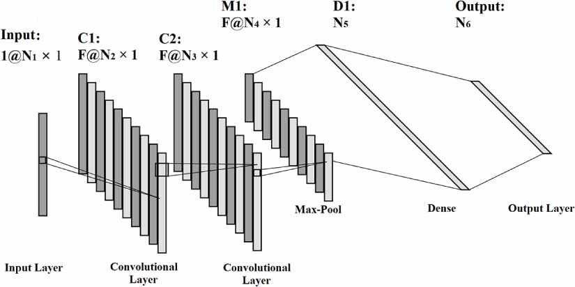
As shown in figure 1, the theoretical architecture of a 1D-CNN model typically consists of several parts: the Input Layer, Convolutional Layer C1, Convolutional Layer C2, Max-Pool Layer M1, Dense Layer D1, and Output Layer.

Figure 1. The Theoretical structure of the 1D-CNN model.
Download figure:
Standard image High-resolution imageIn a 1D-CNN model, the input layer consists of a 1D array with dimensions of  . The subsequent C1 Convolutional layer will have F different feature maps, where each feature map is an array with dimensions of
  . If the kernel size is
  , then their relationship satisfies equation (1)

The Convolutional Layer C2 has a similar structure to the Convolutional Layer C1, with the difference being that N3 is smaller than N2. When the kernel size is  , it satisfies a similar equation:
  . In the Max-pooling layer, if the kernel size is
  , there exists the relation
  . Subsequently, we need to flatten the results to a Dense Layer, and their relationship satisfies
  . Finally, for the Output Layer, its dimension N6 will be the same as the number of different types in the dataset


The equations presented here denote that, in the ath layer and in the bth feature map, the result is obtained at point m along the 1D array. F represents the total number of all the feature maps in the layer of  th. α represents the extended width of the kernel, thus the width of the kernel is
  .
.  represents the activation values in the kernel area of the
  th layer in each of the features, while
  represents the corresponding weights of this specific kernel.
  stands for the bias for the ath layer and the bth feature map. Once we obtain the sum of the weighted values and bias
  , we apply the activation function σ (as equation (3) suggests), so that this result can be converted into
  , which represents the activation value in the ath layer and in the bth feature map.
2.3. 2D-CNN
Figure 2 illustrates the architecture of a 2D-CNN model. Similar to the 1D-CNN model, it consists of several layers, including the Input Layer, Convolutional Layer C1, Convolutional Layer C2, Max-Pool Layer M1, Dense Layer D1, and Output Layer.

Figure 2. The Theoretical structure of the 2D-CNN model.
Download figure:
Standard image High-resolution imageThe 2D-CNN network begins with an input layer that takes in a 2D image with dimensions of  . The first convolutional layer, C1, consists of F kernels with a size of
  , resulting in F feature maps with dimensions of
  , where
  . Similarly, the second convolutional layer, C2, also has F feature maps but with dimensions of
  , where
  , when using a kernel size of
  . For the Max-Pooling layer, with a kernel size of
  , the output size is calculated using
  . The dense layer, D1, has a size of
  , where F is the number of filters and N4 is the output size of the Max-Pooling layer. Finally, the output layer, which corresponds to the number of classification types, has a size of N6


The above equations describe how the result of a specific point (m, n) in the bth feature map of the ath layer is calculated. In the ath layer, F represents the total number of feature maps in the previous layer, which is  th layer. α and β represent the extended width and height of the kernel, respectively. Therefore, the size of the kernel is
  .
.  is the activation value in the kernel area of the
  th layer for the cth feature map.
  is the corresponding weight for this specific kernel.
  represents the bias for the bth feature map in the ath layer. After obtaining the value of
  , which is the sum of the weighted values and bias, the activation function σ (as equation (5)) is applied to obtain the activated value
  in the bth feature map of the ath layer.
2.4. 3D-CNN
Figure 3 illustrates the architecture of a typical 3D-CNN model. This structure typically consists of several layers, including the Input Layer, Convolutional Layer C1, Convolutional Layer C2, Max-Pooling Layer M1, Dense Layer D1, and Output Layer.

Figure 3. The Theoretical structure of the 3D-CNN model.
Download figure:
Standard image High-resolution imageThe input to a 3D-CNN model typically consists of a 3D dataset with the dimensions  . The convolutional layer C1 will have the size of
  . When the kernel used for the convolutional process is of size
  , the following two equations must be satisfied:


The convolutional layer C2 has dimensions of  , with a kernel size of
  between C1 and C2. This requires satisfying the equations
  and
and  . During the Max-Pooling process, with a kernel size of
  , the equations
  and
and  are used to calculate the resulting dimensions. The value of N5 in the Dense Layer D1 is determined by
  . Finally, the number of classification types determines the value of N6 in the Output layer


The equations above show the result of point (m, n, p) in the 3D coordinate system in the ath layer and the bth feature map. F represents the total number of all the feature maps in the  th layer. α represents the extended width of the kernel; thus, the width of the kernel is (1 + 2α). β represents the extended height of the kernel; thus, the height of the kernel is (1 + 2β). γ represents the extended depth of the kernel; thus, the depth of the kernel is (1 + 2γ).
  represents the activation values in the kernel area of the (i − 1)th layer in each feature, while
  corresponds to the weights of this specific kernel.
  represents the bias for the ath layer and the bth feature map. Once we obtain
  , which is the sum of the weighted values and bias, we need to apply the activation function σ (as suggested by equation (9)) to convert this result into
  , which is the activated value in the ath layer and the bth feature map.
3. Proposed method
3.1. Motivation
Hyperspectral datasets contain both spectral and spatial information. However, 1D-CNNs only extract information from the spectral aspect while ignoring spatial information and information among adjacent slices. On the other hand, 2D-CNNs consider spatial information but fail to extract both spectral information and potential information among adjacent slices. To compensate for the disadvantage, we need to use 3D-CNNs, as they are better suited for capturing information among adjacent slices in hyperspectral datasets. In summary, the imperative lies in obtaining more comprehensive results in the process of feature extraction, which is significant in yielding superior and more robust outcomes during subsequent feature fusion and classification. Therefore, it remains essential to conduct a thorough examination of hyperspectral data from all three pertinent aspects to attain this objective.
In addition, even in the applications of former researches that try to combine information from 1D, 2D, and 3D aspects, they fail to explore effective methods for such feature fusion.
This article proposes a new model called attention-based triple-stream fused CNN (ATSFCNN) to address these issues. Firstly, we extract features from HSIs using the techniques of multi-scale 1D-CNN, 2D-CNN, and 3D-CNN. Secondly, we propose a new attention-based feature fusion method to combine features obtained from 1D-CNN, 2D-CNN, and 3D-CNN. Compared with other naive fusions among the features, our fusion method can stress the features which have a higher significance to the results. Furthermore, our model is scalable, as features generated from other neural networks can replace those generated by 1D, 2D, and 3D networks. In that case, our new feature fusion method proposed in this article from 1D, 2D, and 3D networks remains applicable.
3.2. The holistic architecture of ATSFCNN
The architecture of ATSFCNN is shown in figure 4. Its architecture consists of four different modules: Data Preprocessing Module, Feature Extraction Module, Feature Fusion Module, and Output Module.

Figure 4. Architecture of ATSFCNN.
Download figure:
Standard image High-resolution image3.3. Data preprocessing module
The data preprocessing module involves conducting principal component analysis (PCA) on the original hyperspectral dataset to preprocess it. This results in a reduction of the dataset's dimensionality from M×N×P to M×N×L, which serves as input for the 2D stream. In addition, the hyperspectral datacube is transformed into a series of 1D arrays. Each pixel in the 2D (M×N) image is extended in the depth direction, creating M×N 1D arrays. Each array has a dimension of 1×P, which is the input for the 1D stream. The 3D stream uses the original hyperspectral datacube with the size of M×N×P directly.
The choice to use the processed M×N×L datacube for 2D analysis and the original M×N×P hyperspectral datacube for 3D analysis is based on several factors. The 2D approach primarily focuses on 2D spatial information between adjacent pixels, while the 3D approach extracts information primarily from adjacent spectral channels. Therefore, in the case of 3D analysis, it is crucial to retain as many spectral channels as possible, whereas this is not necessary for 2D analysis. In fact, performing PCA on the data before using 2D-CNN can reduce dimensionality, decrease computational workload, and improve classification accuracy. This is demonstrated in later sections by comparing the results of 2D-CNN and 2D-CNN+PCA. As shown in the works of [50], the use of PCA in 2D-CNN can significantly improve HSI classification accuracy.
3.4. Feature extraction module
As depicted in figure 5, the feature extraction module employs the M×N×P dataset directly as input for 3D-CNN. Additionally, the processed M×N×L serves as input for 2D-CNN, while the M×N 1D arrays are used as input for 1D-CNN.

Figure 5. Feature extraction module.
Download figure:
Standard image High-resolution imageIn contrast to the conventional CNN model, our approach uses multi-scale feature extraction. The conventional CNN streams comprise Input_iD, ConviD_1, and ConviD_2 (i = 1,2,3). In our method, Multi-scale Feature_iD_1, Multi-scale Feature_iD_2, and Multi-scale Feature_iD_3 are used for Multi-scale feature extraction. Multi-scale Feature_iD_1 represents the convolutional result of Input_iD using a kernel different from that in ConviD_1. Multi-scale Feature_iD_2 is the concatenation of ConviD_1 and the convolutional result of Input_iD. Finally, Multi-scale Feature_iD_3 is the concatenation of ConviD_2 and the convolutional result of ConviD_1


3.5. Feature fusion module
The feature fusion module, as depicted in figure 6, incorporates multi-scale features extracted from each stream. Equation (13) outlines the fusion process, which employs direct concatenation among the multi-scale features. This approach has been shown to be effective for multi-scale feature fusion, as demonstrated in the explications and experiments conducted in 2022 [51]. Their findings support the efficiency of concatenation for this purpose

Figure 6. Feature fusion module.
Download figure:
Standard image High-resolution image

Deep fusion of features extracted from different dimensions presents a challenge due to differences in their dimensions. To address this, a flattening process is applied to each fused multi-scale feature, which is then passed through the same dense layer. This approach standardizes the extracted features from each stream into a 1D feature array of the same size. Subsequent to the Dense layer, each  (where i assume values of 1, 2, and 3) uniformly assumes dimensions of R × 1, wherein R signifies the extent along the array dimension originating from the Dense Layer

Following the aforementioned standardization process, the fused multi-scale features undergo two subsequent sub-modules: the concatenation permutation module and the attention module.
3.5.1. Concatenation permutation module
The concatenation permutation module is illustrated in figure 7. Given the three streams of extracted features, there are six possible permutations of their concatenation: Fa_1 (1D-2D-3D), Fa_2 (1D-3D-2D), Fa_3 (2D-3D-1D), Fa_4 (2D-1D-3D), Fa_5 (3D-2D-1D), and Fa_6 (3D-1D-2D). The module considers all of these possibilities for concatenation.

Figure 7. Concatenation permutation module.
Download figure:
Standard image High-resolution imageDue to the potential impact of the sequence of concatenation on the accuracy of feature fusion and classification, all six possible combinations of concatenation must be considered. In the experiments, one of these combinations is used at a time, with all six combinations ultimately being utilized

FF_all is the outcome that follows the execution of the Concatenation Permutation Module. Within this module, the three Multi-scale Fused Feature FF_i (R × 1) were concatenated, consequently leading to its dimensions expanding to  .
.
3.5.2. Attention module
In 2017, some reseachers proposed a Transformer model, which marked a significant milestone in the application of attention mechanisms to the domain of images [52]. Their experiments demonstrated the model's ability to enhance significant information and remove redundancy. However, the Transformer model presented in their work was complex, requiring multiple hidden layers. Inspired by this, we propose a lightweight attention-based module in this article that achieves similar results.
As shown in figure 8, the Concatenated Fused Feature (FF_all) is inputted into the Channel Attention and Spatial Attention modules. Our model is inspired by the works of [53], who proposed a similar model of Channel Attention and Spatial Attention. However, there are two key differences between our work and theirs. Firstly, while their model operates solely on 2D images, we have adapted our model to the 1D case for feature fusion among the extracted features of three streams of hyperspectral datasets. Secondly, their models were directly tested on image detection, whereas in our article, we propose a novel and unique application of using the model to improve the classification performance of the fused features.

Figure 8. Attention module.
Download figure:
Standard image High-resolution image3.5.2.1. Channel attention
Channel Attention focuses on the finding out the inter-channel information of the dataset. When constructing our model of Channel Attention, we utilize the Average Pooling as well as Max Pooling.
Initially, during the development of the Channel Attention model, researchers commonly employed Average Pooling as the primary method for feature extraction, as demonstrated in prior works such as [54, 55], which focused on Object Detection and demonstrated the effectiveness of this approach. However, subsequent studies, including [56, 57], have shown that incorporating Max Pooling in addition to Average Pooling can significantly improve model accuracy. Therefore, in the present study, we have opted to utilize both Average Pooling and Max Pooling in our Channel Attention models.
In Channel Attention, the fused feature undergoes both Max Pooling and Average Pooling operations. The outputs of these operations are then passed through a shared network, which generates the respective channel attention maps. To accomplish this, a MLP with a single hidden layer is utilized.
Compared with conventional MLP, a shared MLP is a type of neural network architecture that extracts pertinent features from various inputs, generating intermediate representations that subsequently interface with other facets of the model, such as classifiers or decision-making components. This architectural paradigm embodies the principle of sharing neural network components among diverse data streams, leveraging their collective prowess to amplify the model's overall effectiveness and predictive capacity. The genesis of the Shared MLP can be traced back to pioneering work in the domain of Natural Language Processing in 2017 [58], where its merits were first underscored. Subsequently, this paradigm found extensions in the realm of attention mechanisms [53], augmenting its relevance and utility.
Based on the idea of shared MLP, the process of Channel Attention can be expressed mathematically as shown in equations (16) and (17). CA_map materializes through an automated process that accentuates dominant features while simultaneously reducing the weights of less impactful attributes. Consequently, CA_map corresponds to the features in the FF_all, meticulously representing each feature in a one-to-one correspondence. Thus, the dimensions of the CA_map harmoniously mirror those of FF_all, spanning 


where ⊗ denotes the matrix multiplication.
3.5.2.2. Spatial attention
Spatial Attention focuses on exploiting the inter-spatial information of the dataset. As we have explained in the Channel Attention, in Spatial Attention, we still use the Max Pooling and the Average Pooling at the same time. The main difference is that we concatenate the results of pooling and add a convolutional layer after it for extracting the spatial layer. SA_map emerges as a consequence of an automated procedure that enhances salient features while concurrently diminishing the influence of less impactful attributes. As a result, SA_map impeccably aligns with the individual features present within the FF_all, ensuring a one-to-one representation of each feature. Thus, the dimensions of the SA_map harmoniously mirror those of FF_all, encompassing a spatial span of 


Channel Attention extracts the features more from the aspect of the channel, while Spatial Attention extracts the features more from the aspect of spatial relationship. Even though for 1D case, their difference may not be as distinguishing as the case of 2D. However, it is still useful to consider these two aspects for comprising more comprehensive information

After extracting features from the three streams, their fusion is carried out using equation (20). The resulting fused feature is subsequently utilized in the Output Module for further processing and analysis.
3.6. Output module
The Output Module is where the fused feature FF_Merge, obtained from the Feature Fusion Module as described in section 3.5, is processed using a Dense layer whose size is determined by the number of endmembers present in the dataset being used. This step is critical, as the size of the Dense layer must match the number of endmembers in order to facilitate accurate identification and classification.
3.7. Hyperparameters of models
In previous sections, we discussed the scalability of our ATSFCNN. Specifically, the neural networks used for extracting 1D, 2D, and 3D features can be replaced with other models, and the methods in the Feature Fusion section will still function. However, we must provide further details regarding the structures of the neural networks used in this article.
3.7.1. 1D-CNN
In our conducted experiments, the architecture of the 1D-CNN comprises a total of four hidden layers, as visually delineated in figure 9. The selection of hyperparameters governing this structure entails a multitude of potential permutations. To foster a stringent basis for performance assessment and result in comparability, we opted to standardize the architectural configuration across the 1D-CNN, 2D-CNN, and 3D-CNN models.

Figure 9. The 1D-CNN model in the experiments.
Download figure:
Standard image High-resolution imageCommencing with the foremost convolutional layer, we introduced 64 filters, each characterized by a kernel size of 3×1. The input to this layer is designated as T11. Subsequently, the second convolutional layer integrates 32 filters of identical kernel dimensions, with T12 as its designated input. A subsequent Flatten operation is executed to transform the output into a 1D array, with T13 denoting the resultant array. Consequent to this, a Fully-Connected layer interfaces with the third layer, incorporating a ReLU activation function to exclude non-positive outcomes. This layer assumes dimensions of R×1.
Pertaining to the original hyperspectral dataset with dimensions expressed as M×N×P, as illustrated in figure 4, the dataset's inherent three-dimensional structure is reconfigured into a sequence of 1D arrays. Each individual pixel within the two-dimensional (M×N) image is projected along the depth dimension, yielding M×N distinct 1D arrays. Each of these arrays is characterized by a dimensionality of P×1, which, in turn, serves as the input for the 1D stream. This configuration thus imparts T11 with dimensions of P×1. Given that the kernel dimensions are established at 3×1, in accordance with equation (1), T12 assumes dimensions of (P-2)×1. Similarly, T13 adopts dimensions of (P-4)×1. Within the confines of the Flatten layer, a compression process is initiated, whereby the entirety of the 32 filters within the second convolutional layer are compacted. The outcome of this operation, quantified as (P-4)×32, translates to (32P-128) in numerical terms. Consequently, the resultant output dimensions of the Flatten layer can be succinctly expressed as (32P-128)×1.
The architecture of our 1D-CNN model is primarily inspired by the works of [34, 59], and [60]. However, there is one fundamental difference between our model's architecture and theirs. In their respective studies, they have included a Maxpooling layer. [59, 60] added the Maxpooling layer after all the Convolutional layers, while [34] inserted the Maxpooling layer between the first and second Convolutional layer.
In our study, we decided not to include the Maxpooling layer due to the following consideration. In our 3D-CNN models, the hyperspectral dataset is divided into a series of small cubes measuring 5×5×P, and the kernel is 3×3×3. Without MaxPooling, the 1D-CNN, 2D-CNN, and 3D-CNN can have very similar structures, allowing for better comparison of their individual results. Adding the Maxpooling stage would require much larger small cubes as inputs for the 2D and 3D models. However, this step is not necessary for our study because our primary contribution is proposing a novel method for fusing features from different streams of HSIs for classification purposes.
3.7.2. 2D-CNN
In our conducted experiments, the architecture of the 2D-CNN encompasses a total of four hidden layers, as elucidated in figure 10. Commencing with the foremost convolutional layer, we introduced 64 filters, each characterized by a kernel size of 3×3. The input to this layer is designated as T21. Subsequently, the second convolutional layer integrates 32 filters of identical kernel dimensions, with T22 as its designated input. Subsequently, a Flatten operation is executed, resulting in the transformation of the output into a 1D array, with the resultant array designated as T23. Consequent to this, a Fully-Connected layer interfaces with the third layer, incorporating a ReLU activation function to exclude non-positive outcomes. This layer assumes dimensions of R×1.

Figure 10. The 2D-CNN model in the experiments.
Download figure:
Standard image High-resolution imageWith regards to the original hyperspectral dataset characterized by dimensions M×N×P, as portrayed in figure 4, via PCA, the inherent three-dimensional structure of the dataset undergoes a transformation into a datacube configuration of M×N×L.
In the field of 2D-CNN, it is practical to choose small image patches and use them to represent the class of the pixel in the center of the patches, as discussed by [35]. Specifically, to classify a pixel  at location (x, y) on the image plane, we use a square patch of size s×s centered at pixel
  . To avoid the issue of void values for image patches near the borders, we need to add padding. In this study, we choose to add zero values in the padding parts near the borders of the dataset.
In light of the M×N image being methodically encapsulated within the s×s image patch paradigm as elucidated earlier, it ensues that the input dimensionality pertinent to the 2DCNN-represented by T21-precisely equates to s×s. An intricate facet to underscore is the existence of M×N such minuscule patches that embody the comprehensive representation of the entire dataset. Harmonizing this with the kernel dimensions, as per the precepts of equation (1), culminates in the derivation s-3+1 = (s-2). It follows that T22 attains dimensions denoted as (s-2)×(s-2), with s signifying the size of the image patch. Similarly, T23 assumes dimensions of (s-4)×(s-4), adhering to a parallel rationale.
Within the confines of the Flatten layer, a compression process is initiated, whereby the entirety of the 32 filters within the second convolutional layer are compacted. The outcome of this operation, quantified as (s-4)×(s-4)×32, translates to ( ) in numerical terms. Consequently, the resultant output dimensions of the Flatten layer can be succinctly expressed as (
 )×1.
)×1.
3.7.3. 3D-CNN
In our conducted experiments, the architecture of the 2D-CNN encompasses a total of four hidden layers, as elucidated in figure 11. Commencing with the foremost convolutional layer, we introduced 64 filters, each characterized by a kernel size of 3×3×3. The input to this layer is designated as T31. Subsequently, the second convolutional layer integrates 32 filters of identical kernel dimensions, with T32 as its designated input. Subsequently, a Flatten operation is executed, resulting in the transformation of the output into a 1D array, with the resultant array designated as T33. Consequent to this, a Fully-Connected layer interfaces with the third layer, incorporating a ReLU activation function to exclude non-positive outcomes. This layer assumes dimensions of R×1. Similar to the 2D case, T31 has the size of s×s×s, T32 has the size of (s-2)×(s-2)×(s-2), T33 has the size of (s-4)×(s-4)×(s-4).

Figure 11. The structure of the 3D-CNN model.
Download figure:
Standard image High-resolution image4. Experimental results and discussions
This section will contain the following parts: 4.1 dataset details, 4.2 experimental setup, 4.3 metrics for evaluation, 4.4 baseline results and discussions, 4.5 results for different training/validation/testing proportions
4.1. Dataset details
The study utilizes thr ee hyperspectral datasets: Samson, Urban, and PaviaU. All these three datasets belong to the remote sensing field.
Samson contains 95×95 pixels with 156 channels, covering a wavelength range of 401 to 889 nm with a resolution of 3.13 nm. It includes three different endmembers: Soil, Tree, and Water. Urban comprises  pixels with 162 channels, with a resolution of 10 nm. It consists of six endmembers: Asphalt, Grass, Tree, Roof, Metal, and Dirt. PaviaU has
  pixels with 103 channels. Among all these pixels, only 42 776 pixels belong to the 9 endmembers: Asphalt, Meadows, Gravel, Trees, Painted metal sheets, Bare Soil, Bitumen, Self-Blocking Bricks, and Shadows. These three datasets are all labeled, with ground-truth classification information provided for each pixel.
In these three datasets, 70%, 5%, and 25% are randomly assigned as Training dataset, Validation Dataset, Testing Dataset. The Training dataset assumes a pivotal role as the part for model training. Subsequent to this, the Validation dataset operates as the crucible for refining model hyperparameters. Ultimately, the Testing dataset is enlisted to conduct a comprehensive evaluation of model performance.
The specific dataset partitions are demonstrated in tables 1–3.
Table 1. Classes and number of pixels of Samson Dataset.
| Class Name | Training | Validation | Testing |
|---|---|---|---|
| Soil | 2110 | 151 | 754 |
| Tree | 2566 | 183 | 917 |
| Water | 1641 | 117 | 586 |
Table 2. Classes and number of pixels of Urban Dataset.
| Class Name | Training | Validation | Testing |
|---|---|---|---|
| Asphalt | 13 000 | 929 | 4643 |
| Grass | 24 639 | 1760 | 8800 |
| Tree | 15 728 | 1123 | 5617 |
| Roof | 4778 | 341 | 1707 |
| Metal | 1701 | 122 | 607 |
| Dirt | 6128 | 438 | 2188 |
Table 3. Classes and number of pixels of PaviaU Dataset.
| Class Name | Training | Validation | Testing |
|---|---|---|---|
| Asphalt | 4642 | 332 | 1657 |
| Meadows | 13 054 | 932 | 4663 |
| Gravel | 1469 | 105 | 525 |
| Trees | 2614 | 187 | 933 |
| Painted metal sheets | 942 | 67 | 336 |
| Bare Soil | 3520 | 251 | 1258 |
| Bitumen | 931 | 67 | 332 |
| Self-Blocking Bricks | 2577 | 184 | 921 |
| Shadows | 663 | 47 | 237 |
4.2. Experimental setup
The experiments were conducted using the Anaconda 22.9.0 environment and the Python language, along with the TensorFlow library toolkit. The results were generated on a PC located in the Imaging Department of C2RMF, featuring an Intel(R) Xeon(R) W-2275 CPU 3.30 GHz and an Nvidia GeForce RTX 3080 graphics card, with 128G of memory.
During the validation procedure, we need to determine the most suitable hyperparameters for our model. The two most predominant factors are the learning rate, the value of reduced dimension after PCA. Within this context, for each hyperparameter configuration, models exhibiting maximal classification performance within the validation subset shall be selected. Subsequently, during the assessment conducted on the testing dataset, the chosen model characterized by this specific constellation of hyperparameters will be engaged. During training, the batch size was set to 32, and the Binary Cross Entropy loss function was employed. All experiments utilized the Adam Optimizer, a choice underpinned by Adam's favorable attributes in terms of operational simplicity, invariance of the magnitudes of the parameter [61], excellent performance [62]. The number of epochs was set to 10, and the results of each model were repeated 10 times. The image patch size was fixed at 5 × 5 for all experiments. The experiments were conducted using the same hyperparameters, with a training/validation/testing ratio of 0.70:0.05:0.25.
First, we delve into the calibration of the learning rate, a pivotal facet of utmost significance. The determination of an apt learning rate value assumes paramount importance, as its judicious selection is instrumental in expediting convergence during training. An excessively low value might protract the convergence process significantly, whereas an overly high value can trigger deleterious divergence in the loss function dynamics [63]. In the quest to ascertain the most fitting learning rate, a comprehensive array of options is explored: {0.01, 0.003, 0.001, 0.0003, 0.0001, 0.00 003}. Across these three datasets, the experiments are uniformly executed over a span of 10 epochs. Drawing insights from the classification outcomes vis-a-vis the validation dataset, we identify the optimal learning rate values. For the Samson dataset, the learning rate of 0.001 emerges as the most suitable. Conversely, the Urban and PaviaU datasets manifest an optimal learning rate value of 0.0003.
Secondly, within the framework of our proposed methodology, we introduce an initial application of PCA to effect dimensional reduction in the context of the 2D channel. In this context, the identification of the most appropriate reduced dimension value constitutes a salient endeavor. As depicted in table 4, it becomes evident that for the Samson dataset, optimal performance materializes at a reduced dimension of 15, whereas the Urban dataset attains peak performance at a reduced dimension of 20. Conversely, the PaviaU dataset yields superior results with a reduced dimension of 10. Notably, the tabulated results in table 4 underscore a consistent trend wherein models devoid of PCA preprocessing consistently underperform in comparison to their PCA-incorporated counterparts. This trend resonates with the compelling necessity of integrating PCA as an indispensable facet of the data preprocessing pipeline.
Table 4. OA (%) of different values of reduced dimension after PCA under different datasets.
| Reduced dimension of PCA | Samson | Urban | PaviaU |
|---|---|---|---|
| 5 | 98.31 | 96.94 | 97.34 |
| 10 | 98.45 | 97.07 | 97.47 |
| 15 | 98.76 | 97.23 | 97.36 |
| 20 | 98.39 | 97.38 | 97.25 |
| 25 | 98.34 | 97.35 | 97.22 |
| Without PCA | 97.95 | 96.67 | 96.91 |
4.3. Metrics for evaluation
The metrics used to assess the results of the classification in this section are OA, AA, and κ (kappa coefficient).
The OA is calculated as follows:

Here, Ai represents the number of pixels that belong to the ith class and were correctly classified as the ith class by the model. The variable N represents the total number of pixels in the testing dataset.
The AA is calculated as follows:

Here, Ai represents the number of pixels in the ith class that were correctly classified, and Ni represents the total number of pixels in the ith class. The variable N denotes the total number of pixels in the testing dataset.
κ (kappa coefficient) is a widely used statistical metric, it has been utilized in various fields including medical research [64], classification of thematic map [65], and voice recognition [66]. It is a powerful statistical tool because it is computed by weighting the measured accuracies, which represents the robust measure of the degree of agreement.
According to [67], the κ can be briefly expressed as follows:

where Pr(a) represents the actual observed agreement, and Pr(e) represents chance agreement.
4.4. Baseline results and discussions
In this part, we evaluated the performance of various CNN models for HSI classification on three datasets. The models evaluated included 1D-CNN, 2D-CNN, 2D-CNN + PCA, 3D-CNN, 3D-CNN + PCA, and the proposed ATSFCNN, all implemented in the Python language and TensorFlow library. We used OA, AA, and κ (kappa coefficient) as the evaluation metrics.
The results on the Samson dataset shown in table 5, indicate that the proposed ATSFCNN model outperformed other individual CNN models that use only one stream of the hyperspectral dataset. The OA, AA, and κ results showed that ATSFCNN had the highest OA, AA, and kappa coefficient of classification, as well as the smallest standard deviation compared to other methods. This indicates that the results of ATSFCNN are more stable and consistent, with better prediction ability even for individual classes.
Table 5. Class-specific accuracy (%), overall accuracy (OA), average accuracy (AA), kappa coefficient (κ) and their corresponding standard deviation (%) with different techniques in Samson Dataset.
| Class | 1D-CNN | 2D-CNN | 2D-CNN+ PCA | 3D-CNN | 3D-CNN+ PCA | ATSFCNN |
|---|---|---|---|---|---|---|
| Soil | 96.05 ± 2.04 | 94.32 ± 2.44 | 96.44 ± 1.15 | 96.30 ± 1.52 | 96.08 ± 1.27 | 97.74 ± 0.44 |
| Tree | 99.03 ± 1.63 | 97.96 ± 1.40 | 98.06 ± 0.64 | 97.35 ± 0.90 | 97.35 ± 0.94 | 98.32 ± 0.36 |
| Water | 99.40 ± 0.44 | 98.92 ± 0.60 | 98.56 ± 1.05 | 98.07 ± 1.35 | 98.13 ± 1.16 | 99.37 ± 0.49 |
| OA | 98.05 ± 0.42 | 96.89 ± 0.44 | 97.63 ± 0.25 | 97.13 ± 0.38 | 97.11 ± 0.16 | 98.38 ± 0.11 |
| AA | 98.16 ± 1.84 | 97.06 ± 2.42 | 97.69 ± 1.11 | 97.24 ± 0.89 | 97.18 ± 1.03 | 98.47 ± 0.82 |
| κ | 97.08 ± 0.65 | 95.17 ± 0.72 | 96.37 ± 0.35 | 96.00 ± 0.76 | 95.84 ± 0.40 | 97.41 ± 0.23 |
In table 6, on the Urban dataset, ATSFCNN achieved the highest OA and the smallest standard deviation for the OA metric. Similarly, ATSFCNN outperformed other models in terms of AA and κ. The results in table 7 of the PaviaU dataset also showed that ATSFCNN's performances in OA, AA, and κ were much better than other models, with the highest average and the smallest standard deviation.
Table 6. Class-specific accuracy (%), overall accuracy (OA), average accuracy (AA), kappa coefficient (κ) and their corresponding standard deviation (%) with different techniques in Urban Dataset.
| Class | 1D-CNN | 2D-CNN | 2D-CNN+ PCA | 3D-CNN | 3D-CNN+ PCA | ATSFCNN |
|---|---|---|---|---|---|---|
| Asphalt | 96.74 ± 2.06 | 94.88 ± 0.93 | 95.83 ± 1.77 | 94.95 ± 1.39 | 95.08 ± 2.29 | 97.47 ± 0.87 |
| Grass | 97.02 ± 1.82 | 96.43 ± 0.66 | 96.85 ± 1.09 | 96.23 ± 1.53 | 95.16 ± 1.64 | 97.79 ± 0.40 |
| Tree | 97.98 ± 1.12 | 95.72 ± 0.99 | 95.69 ± 1.4 | 95.12 ± 1.60 | 95.25 ± 2.10 | 98.20 ± 0.75 |
| Roof | 95.66 ± 1.83 | 91.01 ± 2.16 | 92.19 ± 3.76 | 91.03 ± 3.51 | 90.91 ± 3.32 | 95.19 ± 1.68 |
| Metal | 92.87 ± 4.57 | 87.09 ± 6.25 | 90.45 ± 4.08 | 89.73 ± 2.51 | 86.02 ± 3.73 | 92.60 ± 3.94 |
| Dirt | 92.46 ± 4.79 | 86.71 ± 3.27 | 90.81 ± 1.94 | 89.93 ± 3.01 | 89.65 ± 2.24 | 93.56 ± 2.53 |
| OA | 96.47 ± 0.39 | 94.34 ± 0.24 | 95.25 ± 0.48 | 94.53 ± 0.27 | 94.05 ± 0.37 | 97.09 ± 0.16 |
| AA | 95.45 ± 2.29 | 91.97 ± 4.35 | 93.64 ± 2.82 | 92.83 ± 2.92 | 92.01 ± 3.81 | 95.80 ± 0.34 |
| κ | 95.56 ± 0.32 | 93.36 ± 0.36 | 94.04 ± 0.42 | 93.62 ± 0.31 | 93.09 ± 0.38 | 96.14 ± 0.20 |
Table 7. Class-specific accuracy (%), overall accuracy (OA), average accuracy (AA), kappa coefficient (κ) and their corresponding standard deviation (%) with different techniques in PaviaU Dataset.
| Class | 1D-CNN | 2D-CNN | 2D-CNN+ PCA | 3D-CNN | 3D-CNN+ PCA | ATSFCNN |
|---|---|---|---|---|---|---|
| Asphalt | 90.73 ± 3.52 | 92.69 ± 3.25 | 98.24 ± 2.35 | 92.84 ± 1.93 | 80.67 ± 9.70 | 97.48 ± 2.46 |
| Meadows | 94.22 ± 2.43 | 95.62 ± 2.83 | 99.07 ± 1.18 | 97.58 ± 1.21 | 99.17 ± 0.46 | 99.45 ± 0.66 |
| Gravel | 82.91 ± 7.48 | 87.31 ± 5.30 | 98.07 ± 2.25 | 82.15 ± 5.35 | 93.48 ± 3.42 | 90.43 ± 8.90 |
| Trees | 92.10 ± 4.26 | 96.16 ± 4.40 | 90.80 ± 18.88 | 93.49 ± 4.12 | 98.19 ± 1.25 | 95.65 ± 4.02 |
| Painted metal sheets | 99.52 ± 0.47 | 97.37 ± 4.49 | 100.0 ± 0.00 | 88.89 ± 13.49 | 83.18 ± 40.75 | 99.76 ± 0.28 |
| Bare Soil | 83.72 ± 4.34 | 83.24 ± 10.75 | 96.17 ± 7.51 | 89.96 ± 2.17 | 96.87 ± 2.35 | 95.71 ± 3.97 |
| Bitumen | 84.91 ± 6.56 | 85.63 ± 9.92 | 82.21 ± 34.29 | 78.77 ± 12.02 | 86.44 ± 25.55 | 95.37 ± 3.37 |
| Self-Blocking Bricks | 76.11 ± 1.76 | 86.28 ± 7.75 | 67.65 ± 18.14 | 86.49 ± 2.76 | 86.33 ± 10.21 | 89.91 ± 3.79 |
| Shadows | 98.79 ± 1.62 | 99.64 ± 0.87 | 99.64 ± 0.33 | 99.86 ± 0.21 | 80.58 ± 39.71 | 98.49 ± 2.45 |
| OA | 89.92 ± 1.02 | 92.05 ± 1.93 | 92.65 ± 1.81 | 93.02 ± 0.95 | 93.01 ± 1.43 | 96.93 ± 0.89 |
| AA | 89.22 ± 7.86 | 91.55 ± 6.00 | 92.45 ± 10.94 | 89.97 ± 6.80 | 89.43 ± 7.55 | 95.80 ± 3.58 |
| κ | 86.61 ± 1.04 | 89.88 ± 1.09 | 90.06 ± 0.64 | 90.78 ± 0.93 | 91.14 ± 0.91 | 95.21 ± 0.27 |
The illustrations denoted as figures 12–14 revealed the ground-truth results and the corresponding classification maps derived from various methodologies, including 1D-CNN, 2D-CNN, 2D-CNN + PCA, 3D-CNN, 3D-CNN + PCA, and ATSFCNN. The visual representations presented in these figures harmonize cohesively with the numerical values meticulously documented in tables 5–7. Remarkably, even within the context of a testing dataset that encompasses merely a quarter of the entire dataset, the conspicuous excellence of the proposed ATSFCNN model remains distinctly evident, as vividly depicted in table 7.

Figure 12. When the proportion is 70/5/25, classification maps on the Samson dataset obtained by (a) Ground-Truth, (b) 1D-CNN, (c) 2D-CNN, (d) 2D-CNN + PCA, (e) 3D-CNN, (f) 3D-CNN + PCA, and (g) ATSFCNN.
Download figure:
Standard image High-resolution image
Figure 13. When the proportion is 70/5/25, classification maps on the Urban dataset obtained by (a) Ground-Truth, (b) 1D-CNN, (c) 2D-CNN, (d) 2D-CNN + PCA, (e) 3D-CNN, (f) 3D-CNN + PCA, and (g) ATSFCNN.
Download figure:
Standard image High-resolution image
Figure 14. When the proportion is 70/5/25, classification maps on the PaviaU dataset obtained by (a) Ground-Truth, (b) 1D-CNN, (c) 2D-CNN, (d) 2D-CNN + PCA, (e) 3D-CNN, (f) 3D-CNN + PCA, and (g) ATSFCNN.
Download figure:
Standard image High-resolution imageOur study's findings revealed that ATSFCNN, which fuses features from 1D-CNN, 2D-CNN, and 3D-CNN, achieved more accurate and stable predictions than models that use only one stream or part of the hyperspectral dataset. The superior OA of ATSFCNN can be attributed to its architecture, which considers spectral, spatial, and hidden information among adjacent channels in the hyperspectral data. In contrast, individual models such as 1D-CNN, 2D-CNN, and 3D-CNN only capture partial aspects of the data, which can lead to less accurate predictions.
These results demonstrate that, by fusing features from different streams using the attention mechanism, ATSFCNN incorporates information from all relevant aspects, resulting in more stable and accurate predictions with the smallest standard deviation. These results suggest the importance of using ATSFCNN in HSI classification.
4.5. Results for different training/validation/testing proportions
Real-world applications often involve situations where labels are only available for a small proportion of the entire dataset. Therefore, it is crucial to examine the performance of our proposed model, ATSFCNN, under such conditions. To evaluate the robustness of the model, we conducted experiments with different proportions of training, validation, and testing data: 70/5/20, 45/5/50, 20/5/75, 10/5/85, 5/5/90. The notation T1/V/T2 indicates the percentage of the entire dataset used for the training, validation, and testing sets, respectively.
The results presented in table 8 demonstrate that the OA of all methods decreases slightly as the proportion of the testing set increases, which is expected due to the larger proportion of the training set typically leading to better model training. However, ATSFCNN consistently outperforms other methods across various proportions of training/validation/testing, highlighting its potential for real-world applications with limited labeled data. Notably, even when the training dataset accounts for only 5% of the entire dataset, ATSFCNN achieves a high classification accuracy of 96.65%. Furthermore, the relative performance of different methods remains consistent across various proportions of training/validation/testing, with ATSFCNN consistently achieving the highest OA and smallest standard deviation. This consistency suggests that ATSFCNN is a robust model for hyperspectral imaging classification, even in situations where labeled data is scarce.
Table 8. Under different sample proportions, class-specific accuracy (%), overall accuracy (OA) and their standard deviation (%) with different techniques in Samson Dataset
| Proportion | 1D-CNN | 2D-CNN | 2D-CNN+ PCA | 3D-CNN | 3D-CNN+ PCA | ATSFCNN |
|---|---|---|---|---|---|---|
| 70/5/25 | 98.05 ± 0.42 | 96.89 ± 0.44 | 97.63 ± 0.25 | 97.13 ± 0.38 | 97.11 ± 0.16 | 98.35 ± 0.11 |
| 45/5/50 | 97.48 ± 0.77 | 96.60 ± 0.18 | 97.38 ± 0.21 | 96.24 ± 0.54 | 96.55 ± 0.45 | 98.31 ± 0.09 |
| 20/5/75 | 97.28 ± 0.50 | 96.33 ± 0.47 | 96.73 ± 0.31 | 95.20 ± 0.64 | 95.89 ± 0.21 | 98.04 ± 0.16 |
| 10/5/85 | 96.76 ± 1.12 | 95.15 ± 0.71 | 95.59 ± 0.27 | 94.78 ± 0.98 | 95.72 ± 0.94 | 97.20 ± 0.24 |
| 5/5/90 | 96.09 ± 1.00 | 94.54 ± 0.83 | 95.16 ± 0.46 | 94.47 ± 0.57 | 95.11 ± 0.51 | 96.65 ± 0.25 |
Similarly, table 9 presents results of ATSFCNN's performance in predicting the Urban hyperspectral dataset across different proportions of training, validation, and testing data, showing that as the proportion of the training set decreases from 70/5/25 to 5/5/90, ATSFCNN consistently achieves the best OA among all models, with standard deviations that are almost consistently the smallest. Finally, table 10 confirms that ATSFCNN outperforms all other models in predicting Pavia University hyperspectral datasets, irrespective of the proportion of training, validation, and testing data used. These results emphasize the robustness of ATSFCNN in predicting hyperspectral datasets with limited labeled data.
Table 9. Under different sample proportions, class-specific accuracy (%), overall accuracy (OA) and their standard deviation (%) with different techniques in Urban Dataset.
| Proportion | 1D-CNN | 2D-CNN | 2D-CNN+ PCA | 3D-CNN | 3D-CNN+ PCA | ATSFCNN |
|---|---|---|---|---|---|---|
| 70/5/25 | 96.47 ± 0.39 | 94.34 ± 0.24 | 95.25 ± 0.48 | 94.53 ± 0.27 | 94.05 ± 0.37 | 97.09 ± 0.16 |
| 45/5/50 | 95.95 ± 0.44 | 93.60 ± 0.42 | 94.35 ± 0.66 | 93.98 ± 0.34 | 93.35 ± 0.58 | 96.71 ± 0.32 |
| 20/5/75 | 94.99 ± 0.31 | 92.10 ± 0.31 | 92.86 ± 0.64 | 92.25 ± 0.41 | 91.11 ± 0.59 | 95.83 ± 0.20 |
| 10/5/85 | 94.16 ± 0.35 | 90.43 ± 0.52 | 90.76 ± 0.70 | 90.87 ± 0.45 | 88.53 ± 0.69 | 95.39 ± 0.41 |
| 5/5/90 | 93.71 ± 0.75 | 88.81 ± 0.46 | 88.93 ± 0.32 | 89.95 ± 0.69 | 86.62 ± 0.54 | 94.57 ± 0.18 |
Table 10. Under different sample proportions, class-specific accuracy (%), overall accuracy (OA) and their standard deviation (%) with different techniques in PaviaU Dataset.
| Proportion | 1D-CNN | 2D-CNN | 2D-CNN+ PCA | 3D-CNN | 3D-CNN+ PCA | ATSFCNN |
|---|---|---|---|---|---|---|
| 70/5/25 | 89.92 ± 1.02 | 92.05 ± 1.93 | 92.85 ± 1.81 | 93.02 ± 0.95 | 93.01 ± 1.43 | 96.93 ± 0.89 |
| 45/5/50 | 88.05 ± 1.42 | 91.55 ± 1.59 | 92.45 ± 2.83 | 92.48 ± 0.98 | 92.83 ± 1.22 | 96.87 ± 0.93 |
| 20/5/75 | 87.53 ± 1.12 | 91.12 ± 1.40 | 91.90 ± 3.23 | 92.17 ± 1.17 | 92.51 ± 3.33 | 96.72 ± 0.45 |
| 10/5/85 | 86.69 ± 1.40 | 89.81 ± 1.78 | 90.69 ± 1.91 | 90.80 ± 1.42 | 92.22 ± 1.54 | 96.43 ± 0.33 |
| 5/5/90 | 83.72 ± 0.76 | 89.27 ± 1.72 | 90.11 ± 1.90 | 90.23 ± 1.72 | 91.45 ± 1.70 | 95.00 ± 0.46 |
From tables 8–10, two notable trends can be observed regarding the performance of different models on different datasets.
Firstly, the results of 2D-CNN and 3D-CNN fall short of 1D-CNN in the Samson and Urban datasets, while in the PaviaU dataset, this trend is reversed. This can be explained by the fact that 1D-CNN only extracts spectral information, requiring fewer hyperparameters to train the model and being better suited for situations where the number of endmembers is smaller. The Samson dataset has three different endmembers and the Urban dataset has six different endmembers, whereas the number of endmembers in the PaviaU dataset is much larger. Therefore, the simplicity of the 1D-CNN model may provide an advantage over the more complex 2D-CNN and 3D-CNN models in datasets with fewer endmembers.
Secondly, our proposed ATSFCNN consistently outperforms the other models on all three datasets. This can be attributed to the fact that the ATSFCNN incorporates and fuses features extracted from all possible streams, giving it an advantage over other models that only utilize information from one aspect. Additionally, the classification accuracy of ATSFCNN can still be improved by utilizing more complex CNN models with more hidden layers and various scales. However, we emphasize that the main contribution of our research lies in the development of a novel approach for integrating features from all relevant streams, considering all pertinent information from hyperspectral data, and fusing the features for prediction. The specific architectures used for the 1D, 2D, and 3D streams can be substituted with other CNN models, demonstrating the scalability of our proposed ATSFCNN approach.
Figure 15–17 serve as illustrative depictions of the classification maps, which align cohesively with the outcomes as delineated in tables 8–10. Simultaneously, abundance maps corresponding to the authentic ground truths are provided for reference. Notably, the classification maps resulting from the proposed ATSFCNN exhibit markedly reduced levels of noise in various regions, in stark contrast to the outcomes generated by methodologies exclusively reliant on singular streams (1D-CNN, 2D-CNN, 2D-CNN + PCA, 3D-CNN, 3D-CNN + PCA). A specific case in point, as illustrated in figure 17, distinctly underscores the superior classification precision of ATSFCNN in distinguishing between Bare Soil and Self-Blocking Bricks, outperforming all alternative methodologies.

Figure 15. When the proportion is 5/5/90, classification maps on the Samson dataset obtained by (a) Ground-Truth, (b) 1D-CNN, (c) 2D-CNN, (d) 2D-CNN + PCA, (e) 3D-CNN, (f) 3D-CNN + PCA, and (g) ATSFCNN.
Download figure:
Standard image High-resolution image
Figure 16. When the proportion is 5/5/90, classification maps on the Urban dataset obtained by (a) Ground-Truth, (b) 1D-CNN, (c) 2D-CNN, (d) 2D-CNN + PCA, (e) 3D-CNN, (f) 3D-CNN + PCA, and (g) ATSFCNN.
Download figure:
Standard image High-resolution image
Figure 17. When the proportion is 5/5/90, classification maps on the PaviaU dataset obtained by (a) Ground-Truth, (b) 1D-CNN, (c) 2D-CNN, (d) 2D-CNN + PCA, (e) 3D-CNN, (f) 3D-CNN + PCA, and (g) ATSFCNN.
Download figure:
Standard image High-resolution image
5. Conclusions
This study addresses two critical limitations of existing research in the classification of HSIs, namely the absence of consideration of 3D information and studies on feature fusion. To overcome these limitations, we present a novel Convolutional Network model, ATSFCNN, which utilizes a novel attention-based feature fusion method to fuse features extracted from hyperspectral datasets in 1D, 2D, and 3D dimensions.
We conducted experiments on three remote sensing datasets to compare the performance of ATSFCNN against other CNN models that use only one stream, including 1D-CNN, 2D-CNN, 2D-CNN+PCA, 3D-CNN, and 3D-CNN+PCA. Our results indicate that, ATSFCNN always outperforms all other models across different training/validation/testing proportions in the average of OA. And ATSFCNN obtains the smallest in the standard deviation of OA for almost all the cases. In fact, even when it does not achieve the smallest standard deviation of OA, its value remains comparable to that of the best-performing models. Significantly, our proposed ATSFCNN model demonstrates superior stability and robustness, essential attributes for real-world applications.
Our experiments demonstrate that ATSFCNN's performance is not only superior in terms of accuracy but also in terms of stability, which is a crucial consideration for developing reliable models applicable to various scenarios and datasets. The consistently superior performance of ATSFCNN in terms of stability, as demonstrated by the small standard deviation in the results, further supports its reliability.
Overall, our study establishes that ATSFCNN is an effective approach for HSI classification. By integrating features from various CNN models, ATSFCNN captures and utilizes information from different aspects of hyperspectral data, leading to enhanced accuracy and stability. This approach holds potential for further extensions and adaptations to other datasets and applications in the future.
Acknowledgment
This work has received funding from the European Union's Horizon 2020 research and innovation program under the Marie Skłodowska-Curie Grant Agreement No. 813789.
Data availability statement
The data that support the findings of this study are openly available at the following URL/DOI: https://github.com/jizhencai/dataPublication.