

Abstract
Aircraft condensation trails, also known as contrails, contribute a substantial portion of aviation's overall climate footprint. Contrail impacts can be reduced through smart flight planning that avoids contrail-forming regions of the atmosphere. While previous studies have explored the operational impacts of contrail avoidance in simulated environments, this paper aims to characterize the feasibility and cost of contrail avoidance precisely within a commercial flight planning system. This study leverages the commercial Flightkeys 5D algorithm, developed by Flightkeys GmbH, with a prototypical contrail forecast model based on the Contrail Cirrus Prediction (CoCiP) model to simulate contrail avoidance on 49 411 flights during the first two weeks of June 2023, and 35 429 flights during the first two weeks of January 2024. The utilization of a commercial flight planning system enables high-accuracy estimates of additional cost and fuel investments by operators to achieve estimated reductions in contrail-energy forcing and overall flight global warming potential. The results show that navigational contrail avoidance will require minimal additional cost (0.08%) and fuel (0.11%) investments to achieve notable reductions in contrail climate forcing (−73.0%). This simulation provides evidence that contrail mitigation entails very low operational risks, even regarding fuel. This study aims to serve as an incentive for operators and air traffic controllers to initiate contrail mitigation testing as soon as possible and begin reducing aviation's non- emissions.
Export citation and abstract BibTeX RIS

Original content from this work may be used under the terms of the Creative Commons Attribution 4.0 license. Any further distribution of this work must maintain attribution to the author(s) and the title of the work, journal citation and DOI.
Acronyms

|
 equivalent equivalent |
| EF | energy forcing |

|
 energy forcing energy forcing |

| contrail energy forcing |
| EIn | soot number emissions index |
| RF | radiative forcing |

| Carbon Dioxide |
| AAL | American Airlines |
| aCCFs | Algorithmic Climate Change Functions |
| aGCMs | Atmospheric General Circulation Models |
| APCEMM | Aircraft Plume Chemistry Emission and Microphysics |
| ATC | Air Traffic Control |
| ATM | Air Traffic Management |
| B2B | Business-to-Business |
| CoCiP | Contrail Cirrus Prediction |
| ECMWF | European Centre for Medium-Range Weather Forecasts |
| ETD | estimated time of departure |
| FK5D | Flightkeys 5D |
| GFS | Global Forecast Systems |
| GWP | Global Warming Potential |
| HRES | High-resolution |
| ISSR | ice supersaturated regions |
| KPIs | key performance indicators |
| NOTAMS | Notice to Airmen |
| nvPM | non-volatile particulate matter |
| OEMs | original equipment manufacturers |
| SAC | Schmidt-Appleman criterion |
| SAF | Sustainable Aviation Fuel |
| TH | time horizon |
| USA | United States of America |
| USD | U.S. Dollars |
1. Introduction
The environmental impact of commercial aviation has gained significant attention as a prominent industry challenge. While studies of aviation's climate impacts have primarily focused only on carbon dioxide ( ) emissions, recent research has highlighted the importance of non-
 emissions, particularly nitrogen oxides (NOx), water vapor, and aerosols (soot and sulfates) [1–3]. In certain atmospheric conditions, exhaust heat, water vapor, and aerosols mix with the background atmosphere to form condensation trails (contrails) [4]. In ice-supersaturated regions of the atmosphere, contrails can persist and expand into contrail cirrus clouds.
Contrail cirrus plays a significant role in altering the Earth's energy balance, resulting in temperature change. High-altitude ice clouds, including natural and contrail-induced cirrus clouds, strongly absorb outgoing thermal (longwave) radiation while only minimally reflecting incoming solar (shortwave) radiation [5, 6].
In areas of high air traffic density, such as central Europe and the USA East Coast, contrail cirrus can cover up to 10% of the sky area, exerting a considerable impact on the regional radiative balance [7]. Unlike  forcing, which spreads evenly due to
  's long lifetime, the climate impact caused by contrail cirrus exhibits spatial and temporal variability, influenced by time of day, local meteorology, surface and cloud albedo, and air traffic density [8–10].
Multiple strategies have been proposed to reduce the climate impacts of contrails. Alternative fuels, such as SAF or e-Fuels, are expected to alter contrail properties and reduce contrail lifetimes [11, 12]. Alternative propulsion sources, such as hydrogen or electric aircraft, change engine emissions and can reduce or remove contrail formation altogether. This paper focuses on navigational avoidance, a short-term contrail mitigation option with strong potential, where contrail impacts are reduced by rerouting aircraft around predicted or observed contrail-forming regions.
Many studies have modeled the formation and avoidance of contrails based on weather and climate models, such as the CoCiP model [9, 13], the APCEMM model [11], aGCMs [14–16], or the aCCFs [17, 18], to name a few. Contrail formation and evolution can also be observed directly from ground and satellite imagery [19–21]. Recent advancements in machine learning have enabled contrails to be automatically detected from geostationary satellite imagery [22, 23], enabling large-scale comparison with contrail predictions [24, 25].
While further studies are required to assess the accuracy and efficacy of contrail forecast models [26–28], this study seeks to understand the costs and feasibility of contrail avoidance from an operations perspective, assuming accurate avoidance regions are available. This paper utilizes a prototypical contrail forecast model based on the CoCiP model publicly available through the Contrails API [29, 30].
Several studies have analyzed the feasibility of contrail-optimal trajectory generation in different airspace scenarios using historical flight data [17, 31–36]. It was not until [37] that a commercial flight planning system was used to evaluate the actual operational risks of pre-tactical avoidance. Building upon the methods in [37], the current study analyzes 84 839 AAL flights (a customer of Flightkeys) representing over four weeks of operations globally during the months of June 2023 and January 2024.
The objectives of this study are threefold:
(i) demonstrate an implementation path for contrail forecast data in commercial flight planning tools; (ii) analyze the operational impact of contrail avoidance on a significant number of flights (84 839) operated by AAL, including changes in cost, flight time, fuel consumption, and estimated climate impacts; (iii) compare the results of the winter and summer analyses to comprehend the seasonal impact of contrail avoidance on airline operations.
2. Methods
This section outlines the algorithms, models, and data interfaces used in the study.
Section 2.1 introduces Flightkeys GmbH and its optimization tool, FK5D. Section 2.2 provides an overview of the contrail models used to estimate the climate impact of individual flights and define avoidance regions for the optimizer. Section 2.3 introduces contrail climate metrics and how this study compares the climate impact of contrails with  . Section 2.4 reviews the experimental design and key output metrics.
2.1. FK5D
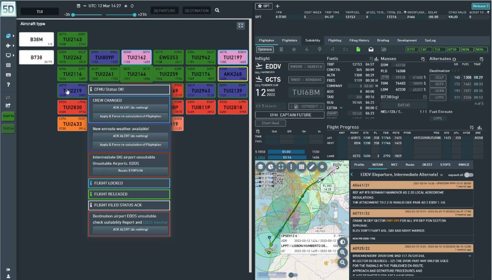
This study leverages the commercial FK5D platform to perform trajectory optimization, trajectory validation, and total cost evaluation. FK5D is developed by Flightkeys 5 , a provider of cloud-based flight platforms, founded in 2015 and based in Vienna, Austria. FK5D provides real-time flight tracking, fuel management, maintenance management, and flight data analysis capabilities, accessible through a web interface. A screenshot of FK5D is shown in figure 1.
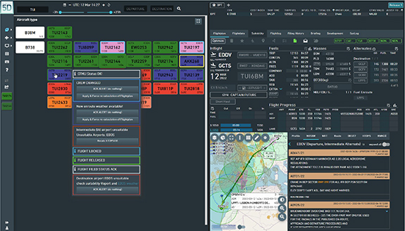
Figure 1. Screenshot of the FK5D platform.
Download figure:
Standard image High-resolution imageThe FK5D trajectory optimizer uses a combination of two established path-finding algorithms from the field of computer science: Dijkstra's algorithm and the A* algorithm [38]. FK5D's optimization problem aims to find the flight plan with the minimum cost. The optimizer considers fuel requirements, weather conditions, and aircraft performance as part of the heuristic cost function. FK5D calculates the cost-optimal flight plan in real-time within a cloud-based environment. Specific implementation details of the FK5D optimizer algorithm are proprietary and cannot be disclosed due to its intellectual property status.
FK5D employs high-resolution aircraft performance data, furnished directly by the OEMs for each unique airframe-engine configuration. OEMs can improve aircraft performance estimates using tail-specific correction factors. FK5D calculates high-fidelity true airspeed and aircraft mass estimates as inputs to the contrail models described in section 2.2.1. For meteorology, FK5D uses NOAA's GFS upper-air weather forecasts for wind and temperature, following standard protocols in airline operations. Meteorology data is interpolated on a 6 h temporal grid, a 1.25∘ lateral grid and different flight levels 6 .
FK5D includes a dynamic, global navigational database of waypoints, airways, airports, terminal routes, and variable restriction data. Restrictions include airspaces, conditional restrictions, and mandatory routes, as published in NOTAMS and specialized B2B platforms.
For the financial comparison of the trajectories generated in this study, FK5D uses the following cost metrics:
- Fuel Cost: The system utilizes an average fuel price of 1.15 USD kg−1.
- Time Cost: Time-dependent costs such as maintenance and leasing are assigned to each aircraft type. Delay costs are omitted for this study since we assume flights take off at the provided estimated time of departure (ETD).
- Overflight Charges: The trajectory optimization process calculates precise, country-specific, and aircraft-specific overflight charges.
2.2. Contrail models
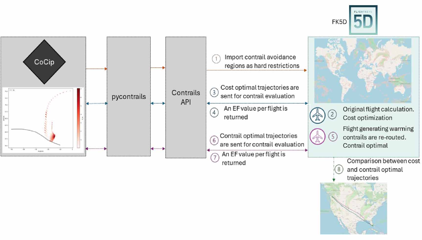
Two types of contrail models are used in this study: (1) a trajectory model that estimates the contrail climate forcing of an individual flight; and (2) a forecast model that predicts avoidance regions expected to form strongly warming contrails on a regular grid. Figure 2 illustrates illustrates how both models are used in combination with FK5D.
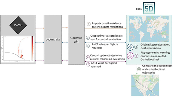
Figure 2. Schematic workflow of contrail avoidance regions import and contrail evaluation and recalculation using the pycontrails library and the FK5D flight planning tool.
Download figure:
Standard image High-resolution image2.2.1. Trajectory model
We use the CoCiP model to estimate contrail climate forcing of individual flight trajectories before and after optimization in FK5D [9, 13]. CoCiP is a parameterized physical model that efficiently estimates formation, persistence, and climate forcing of contrail segments produced by flights. The details of CoCiP are described elsewhere in the literature [6, 10, 39, 40] and available as part of the open-source pycontrails 7 library [30]. Figure 2 (3, 4, 6, 7) illustrates trajectory evaluation with pycontrails using the CoCiP model.
Briefly, CoCiP initializes contrail segments when two adjacent flight waypoints satisfy the SAC [4, 41]. Segments are considered persistent if contrail ice particles survive the initial wake vortex phase. Persistent segments evolve in time using a Runge–Kutta integration scheme until the contrail segment reaches an end-of-life criterion. Contrail end of life is defined as when the ice number concentration is lower than the background ice nuclei ( ), contrail optical depth (τcontrail) is less than 10−6, or the contrail segment reaches a maximum age of 12 h.
FK5D runs CoCiP through the Contrails API
8
[29] (figure 2 points 3, 6), a hosted version of pycontrails with built-in meteorology data available through an HTTP interface. This study ran the Contrails API version v0.15.6 with pycontrails version v0.42.1 [30]. This version of the API included ECMWF HRES meteorology forecast data as input to the CoCiP model. At the time of this study, HRES data was available through the Contrails API hourly out to +36 h for pressure levels
9
on a  latitude-longitude grid. The specific humidity variable of the ECMWF HRES forecast is scaled using the methodology described in [42].
CoCiP uses jet engine emissions, in particular nvPM soot number emissions index (EIn ), to estimate initial ice crystal activation in the contrail plume. pycontrails implements models for nvPM EIn emissions based on aircraft, engine type, and aircraft performance as described in [12, 43]. FK5D provides high-fidelity true airspeed and aircraft mass estimates calculated with proprietary coefficients from the airline to override the standard aircraft performance models built into pycontrails (see section 2.1). One exception is overall propulsive efficiency, which is not provided by OEMs datasets. For this metric, FK5D relies on the default aircraft performance relations implemented in pycontrails, described in detail in [43].
2.2.2. Avoidance regions
To estimate regions that have the potential to form strongly warming contrails, we use a generalized form of the CoCiP model (termed CocipGrid) that calculates contrail climate forcing for arbitrary vector pseudo-waypoints independently [44]. In this formulation, each waypoint represents a nominal flight segment placed at the center of the vector coordinate. Aircraft performance and emissions are estimated assuming a single aircraft-engine combination and nominal cruising conditions at each vector waypoint. Any contrail formed by the nominal segment is evolved as in the original CoCiP model, independent of segments placed at other vector waypoints.
The output of the CocipGrid model is a field of contrail climate forcing per flight distance at each vector waypoint. When the model is evaluated using forecast meteorology, the output can be interpreted as a forecast of expected contrail climate forcing for a specific aircraft flying nominal cruise conditions through a grid cell. While output accuracy is currently limited by known challenges in forecasting upper tropospheric humidity [25, 26, 28], this output effectively emulates the size and distribution of contrail forecast data for the purposes of quantifying cost and avoidance feasibility.
CocipGrid is part of the pycontrails library and used to serve prototypical contrail forecasts through the Contrails API. Forecasts are generated every 6 h out to +36 h using the latest ECMWF HRES meteorology forecast for a set of 10 standard aircraft. To simplify this study, we use forecast data generated for only one aircraft-engine combination (A320). In the future, we expect contrail forecasts to incorporate aircraft-engine dependencies. Forecast data is initially calculated on the native HRES resolution
10
and then linearly interpolated in altitude to flight levels 28 000  (FL280) to 41 000
  (FL410) in 1000
  steps and down-sampled to a
  latitude longitude grid.
Contrail forecasts are served through the Contrails API in two formats: (1) as a NetCDF file containing a single continuous variable of climate forcing per flight distance or (2) as a GeoJSON format containing polygon isolines of climate forcing at each flight level. Polygons are calculated using a threshold of  J m−1 chosen based on the results of a global contrail simulation for 2019–2021 [42, 45]. For this simulation, the contrail polygons are calculated and then ingested into FK5D navigation service database as hard restrictions (figure 1 point 1). The threshold chosen for this study reflects the 80th percentile of contrail climate forcing per flight distance in the global simulation [42]. This study does not explore the impact of the polygon threshold on route modification and overall cost, but this is an important area of future work.
2.3. Contrail metrics
This subsection describes the metrics commonly used to quantify contrail climate forcing in terms of RF and EF, and outlines the method to approximate the contrail cirrus GWP and estimate contrail warming impact as CO2 equivalent (CO ) emissions.
RF, measured in W m−2, represents the net instantaneous change in energy flux at the top of the atmosphere per unit area caused by a contrail [46]. While RF is often presented as a total energy flux averaged over the surface of the Earth over the course of a year, RF in the context of this study refers to the spatial and time extent of an individual contrail.
The integrated RF of a contrail segment over its lifetime is termed the contrail energy forcing (EF ). EF
). EF , measured in J (or J m−1 when normalized by flight distance), quantifies the total energy trapped by a contrail within the atmosphere. EF
 is calculated by integrating the contrail RF over the length (L), width (W), and lifetime (t) of the contrail, as represented by equation (1) [47],

While there is an active debate on metrics for comparing short and long-lived climate pollutants, EF enables us to compare the energy stored by contrails with the energy stored by  emissions over a certain time period. We can quantify the CO2 energy forcing (EF
 ) from jet fuel over a TH [6] as,
where  represents the total fuel consumption in kg,
  is the emission index for
  (
( ), SEarth is the surface area of the Earth (
 ), and
  is the absolute global warming potential for
  over a selected TH. The calculation of
  takes into account the
  radiative forcing due to emission pulses over the chosen time horizon, as well as the decay in
  radiative forcing over time [48]. Table 1 shows
  values for different TH as calculated by [49].
Table 1.
 values for different TH as calculated by [49].
| TH | Units | Values |
|---|---|---|

| yr W m−2 kg CO2 |
![$92.5\ [68, 117]\times 10^{-15}$](https://content.cld.iop.org/journals/2634-4505/4/1/015013/revision3/erisad310cieqn40.gif)
|

| yr W m−2 kg CO2 |
![$25.2\ [20.7, 29.6] \times 10^{-15}$](https://content.cld.iop.org/journals/2634-4505/4/1/015013/revision3/erisad310cieqn42.gif)
|
To compare the expected warming impact between contrails and  , we estimate an
  conversion factor of 0.42 [3, 42],

The choice of time horizon for GWP evaluation crucially shapes environmental strategies in aviation. A 20 yr horizon emphasizes short-term effects, useful for addressing rapidly changing phenomena like contrail cirrus. Conversely, a 100 yr horizon provides a long-term view, focusing on sustained greenhouse gas effects. For instance, in [3], the  of contrail cirrus in 2018 (based on a Tg
  basis) is 2.32, whereas for
  , it is 0.63.
This study uses a 20 yr time horizon by default. The authors acknowledge this choice should reside in the realm of policy and therefore include a comparison of results over alternate time horizons in section 4.1.
2.4. Experimental design
2.4.1. Flight selection
This study includes the analysis of 84 839 AAL flights conducted during two seasons: one in summer, encompassing flights departing between 3 and 18 June 2023; and another in winter, covering flights taking place between 3 and 18 January 2024. Of the 49 411 summer flights, 39 691 are domestic flights within the USA, while 9723 are international. Of the 35 429 winter flights, 27 454 are domestic, while 7920 are international.
Flight data includes regular flights to various countries in South America, Europe, and East Asia. The most frequent international destinations include Mexico, the United Kingdom, and the Dominican Republic. More details on the flight dataset are included in

Figure 3. Maps of domestic and international flights simulated in this study.
Download figure:
Standard image High-resolution image2.4.2. Contrail avoidance simulation
Contrail avoidance regions are generated every 6 h by the CocipGrid model using ECMWF HRES forecast data (section 2.2) out to +36 h. Every hour, FK5D imports new contrail avoidance polygons as restrictions by calling the Contrails API (figure 2, point 1).
Each evening, FK5D imports flights scheduled for the following day and creates optimal trajectories according to the default customer settings. Flights are first calculated without contrail avoidance as a basis for comparison (figure 2, point 2). After the first calculation, FK5D automatically runs each trajectory through the /trajectory/cocip endpoint of the Contrails API to estimate the EF for each segment of the route (figure 2, point 3).
The total net EF of the trajectory is calculated by summing the EF
 of each segment (figure 2, point 4). Flights that generate net warming contrails (
 EF
EF ) are automatically re-routed around the contrail avoidance regions implemented as polygon restrictions (figure 2, point 5). While the optimizer does consider ATM restrictions, the post-calculation filing of flights and subsequent validation of trajectory feasibility is not simulated. Flights were selected for rerouting based on their contrail warming potential [50, 51].
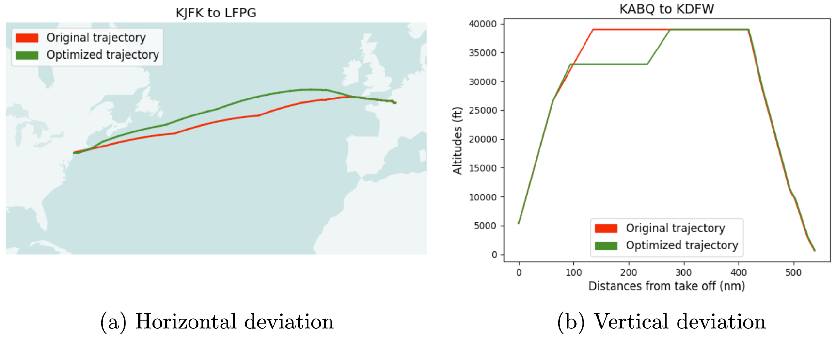
The optimization is performed vertically, laterally, or a combination of both, depending on the most cost-effective solution (figure 4). Once re-optimization is complete, each new trajectory is rerun through the Contrails API to obtain an updated EF for the modified trajectory (figure 2, points 6–7). The final step involves comparing the cost-optimal and contrail-optimal flights (figure 2, point 8).

Figure 4. Examples of contrail avoidance through vertical and horizontal deviations.
Download figure:
Standard image High-resolution image2.4.3. Key output metrics
The simulation employs flight data from Flightkeys' customer, AAL. This data includes origin-destination pairs, flight schedules, payload, cost index, and aircraft types for all simulated flights. To approximate real-world scenarios as closely as possible, aircraft performance metrics used by the airline were imported into our testing environment from the customer's production environment. While the initial flight data import is the same in both environments, the final trajectory flown might differ due to last-minute changes in flight data or routing decisions made by the flight dispatchers after the initial data import.
Upon trajectory calculation, the system evaluates several key performance indicators (KPIs), including trip fuel, measured in kilograms (kg); total cost of operation (including overflight costs), in U.S. Dollars (USD); and flight duration, in minutes. For each trajectory, positive and negative contrail EF values in megajoules (MJ) are retrieved and stored from the Contrails API.
The principal aim of this study is to characterize the trade-offs between these KPIs, EF , and GWP. Ultimately, the analysis seeks to pinpoint scenarios wherein reductions in EF
 (and combined EF
 + EF
+ EF ) can be achieved with the least impact on other KPIs.
3. Results
This section presents the simulation results of the original (cost optimal) and re-optimized (contrail optimal) flight trajectories for the combined set of summer and winter flights. A breakdown by season is presented in section 4.1. Section 3.1 reviews the statistics and climate forcing of the original flights. Section 3.2 presents the results of re-optimizing flights around contrail regions and explores methods for down-selecting interventions to minimize added costs.
3.1. Cost optimal trajectories
The original flight dataset contains 84 839 AAL flights, 49 411 of them operated during a 15-day period in June 2023 and 35 428 operated during a 15-day period in January 2024. The original operational statistics are shown in table 2.
Table 2. Flight statistics and climate impact assessment of all 84 839 flights before and after contrail re-optimization.
| Statistics | Units | Cost optimal | Contrail optimal | Δ (%) |
|---|---|---|---|---|
| Number of flights | — | 84 839 | 84 839 | 0 |
| Flights forming persistent contrails | — | 20 065 (23.7%) | 17 474 | −12.9% |
| Flights forming net warming contrails | — | 11 620 (13.7%) | 8562 | −26.3% |
| Flights forming net neutral or cooling contrails | — | 8445 (10.0%) | 8912 | 5.5% |
| Total flight time | 103 hr | 209.6 | 209.6 | 0.00% |
| Total fuel burn | 109 kg (Mt) | 0.660 | 0.661 | 0.11% |
| Total cost | 106 $ | 1285 | 1286 | 0.08% |
Total  emissions emissions | 109 kg (Mt) | 2.086 | 2.089 | 0.11% |
Total EF
| 1018 J | 0.874 | 0.236 | −72.95% |
Flights responsible for 80% EF
| % | 1.572 | — | — |
Contrail warming, in 
| 109 kg (Mt) | 0.906 | 0.245 | −72.95% |
Total warming, in 
| 109 kg (Mt) | 2.992 | 2.334 | −22.00% |
The flights collectively consumed  (0.66 Mt) of fuel, which for jet fuel
  emissions index
  [52] releases
  kg (2.1 Mt) of
  emissions.
Of the 84 839 original flights, CoCiP predicts 20 065 flights (23.7% of the total) form persistent contrails with non-zero EF . Of these contrail-forming flights, 11 620 flights (13.7%) generate net warming contrails, while 8445 (10.0%) generate net cooling contrails. These figures are broadly consistent with global contrail simulations conducted for the years 2019–2021 [42].
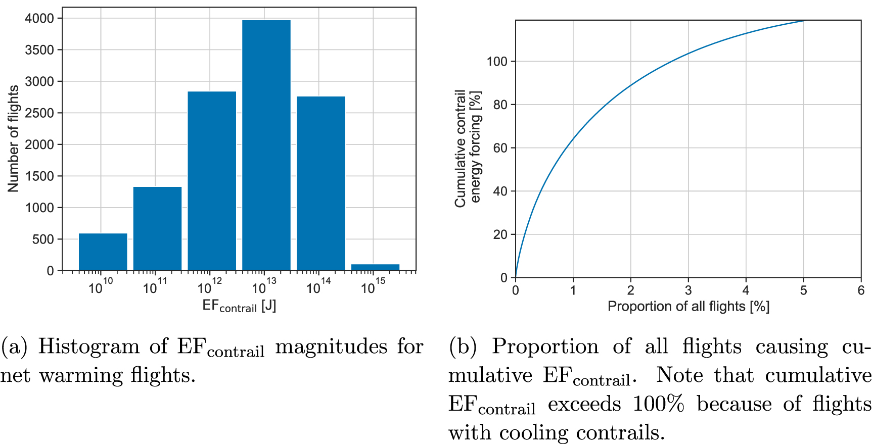
Figure 5(a) shows the EF distribution for net warming flights. Figure 5(b) shows the cumulative contrail energy forcing caused by a specific portion of the total flights. Because of the logarithmic distribution of forcing, we find that 1.57% of flights cause 80% of the EF
 , similar to previous estimates [10, 42, 46].

Figure 5. Proportion of original flights generating contrails, and the EF distribution.
Download figure:
Standard image High-resolution imageUsing equations (2) and (3) (section 2.3), the total contrail forcing can be roughly transformed to  (Mt). Given
  kg
kg  emissions, contrails constitute roughly 30.3% of the climate forcing of the original flight trajectories. If we considered a 100 yr time horizon, contrails would be responsible for 10.6% of the total climate warming (refer to section 4.1).
Table 2 provides a summary of the original flight statistics and climate forcing before re-optimization.
3.2. Contrail optimal trajectories
Out of a total of 20 065 flights that generated persistent contrails, 11 620 flights were selected for re-optimization because they formed net warming contrails ( EF
EF ). Given that contrail avoidance areas were imported as hard constraints, the optimizer failed to find a viable solution in 709 cases (6.1%). Consequently, only 10 911 were successfully re-routed.
After re-optimization, the number of flights generating persistent contrails decreased from 20 065 to 17 474, and the number of flights forming net warming contrails reduced by 26.3%. The total sum of EF reduced 72.95% to
  J. The overall fuel consumption increased by 0.11%, total flight time remained unchanged, and overall costs increased by 0.08%. In accordance with the fuel increase, total
  emissions rose by 0.11%. Table 2 provides overall statistics for the original and re-optimized set of flights.
3.2.1. Selecting interventions
In this section, we explore two heuristic approaches to identify flights to prioritize for rerouting. The first heuristic aims to minimize EF with minimal flight modifications (target big hit flights); the second prioritizes maximizing the ratio of EF
 change to added cost (target low cost reroutes).
3.2.1.1. Targeting big hit flights
The studies reported in [6, 10, 42] present the concept that a small subset of flights, roughly 2%–10%, cause approximately 80% of the total contrail forcing. The results of this study show a similar lever for targeting flights with outsize climate forcing (section 3.1, figure 5(b)). This approach aims to address the majority of climate benefits while minimizing the number of modified flights and, therefore, operational disruptions. Reducing the total number of modifications reduces the total fuel and time costs as well as the workload for ATC.
One way to implement this concept in practice is to only re-optimize flights with the original  EF
EF above a certain threshold. To determine the appropriate value for this threshold, we can sort the original flight data by descending
  EF
EF and find the flight with the
  EF
EF where the curve crosses 80% of the total possible reduction. Figure 6 displays the change in total contrail EF, fuel consumption, cost, and time as a function of the original
  EF
EF sorted from the highest to the lowest.
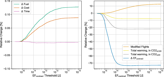
Figure 6. Relative change in total fuel, cost, and time (left); and number of modified flights, EF and total warming in
  and
and  (right) when selecting interventions by original flight EF
 .
.
Download figure:
Standard image High-resolution imageThe  EF
EF threshold for the flights responsible for 80% of the total warming EF
 is
is  J. There are 2438 flights exceeding this threshold, representing 2.87% of the total flight count. The optimizer was able to identify alternative routes for 2260 of these flights. The results of rerouting this subset of flights are detailed in table 3. Compared to the original set of flights, the total contrail EF is reduced by 65.68% with only 0.05% added fuel and 0.03% added cost.
Table 3. Flight statistics for targeting big hit interventions and comparison with full optimization scenario.
| Statistics | Units | Cost optimal | Big hits | Δ (%) |
|---|---|---|---|---|
| Number of flights | — | 84 839 | 2260 | — |
| Time | 103 hr | 209.6 | 209.6 | 0.00% |
| Fuel | 109 kg (Mt) | 0.660 | 0.661 | 0.05% |
| Cost | 106 $ | 1285 | 1286 | 0.03% |
Total  emissions emissions | 109 kg (Mt) | 2.086 | 2.087 | 0.05% |
| Total EF contrail | 1018 J | 0.874 | 0.300 | −65.68% |
Contrail warming in 
| 109 kg (Mt) | 0.906 | 0.311 | −65.68% |
Total warming, in 
| 109 kg (Mt) | 2.986 | 2.398 | −19.85% |
Even though in the example, we focus on the top 2.87%, other possible selection strategies could be considered. Rerouting can be performed based on a contrail EF threshold value or on pre-determined geographical or seasonal/hourly criteria (see section 4.1.2), as discussed in [10, 53]. This criterion could be further strengthened by incorporating a probability ratio; the higher the probability of a flight generating contrails, the greater the likelihood of rerouting. The probability could be assessed by comparing the agreement of different models over a specific contrail forecasted area.
3.2.1.2. Targeting low-cost re-routes
While the previous method aims to limit the number of modified flights, an alternate strategy is to target the most cost-effective re-routes. Airlines can set a specific cost threshold and all flights with rerouting costs below this threshold will be selected for optimization.
The first step involves determining the specific cost, measured in USD, per unit of total warming (accounting for both contrails and  ) in tonnes of
  (T
(T ). This specific cost for each flight is quantified as:

Figure 7 shows the reduction in contrail EF as a function of specific cost. Notably, roughly 10% reduction in EF can be achieved at minimal added cost. Above these low-cost interventions, EF
 reductions show a similar trend to targeting bit hit flights, dropping steeply and then leveling off beyond a specific investment. This shape indicates an optimal cost range, where most reduction in EF
 is achieved for a moderate investment.
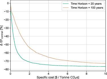
Figure 7. EF reduction for specific cost calculated for 20 yr and 100 yr time horizons.
Download figure:
Standard image High-resolution imageThe decision on investment allocation rests with airlines and policymakers. In contrast to the previous section, where the focus was on modifying a minimum number of flights, the specific-cost approach focuses on rerouting the most economically efficient flights, thereby minimizing added fuel. As an example, we could apply a specific cost threshold of 0.5 USD per tonne of  to this simulation data. In this scenario, 2438 flights, constituting 2.87% of the total, would be re-routed. The operational and environmental implications stemming from these reroutings are detailed in table 4.
Table 4. Flight statistics for targeting low specific cost interventions for a cost threshold of 0.5 USD/tonne of  and comparison with full optimization scenario.
| Statistics | Units | Cost optimal | Low-cost | Δ (%) |
|---|---|---|---|---|
| Number of flights | — | 84 839 | 2438 | — |
| Time | 103 hr | 209.6 | 209.6 | 0.00% |
| Fuel | 109 kg (Mt) | 0.660 | 0.661 | 0.02% |
| Cost | 106 $ | 1285 | 1286 | 0.01% |
Total  emissions emissions | 109 kg (Mt) | 2.086 | 2.087 | 0.02% |
| Total EF contrail | 1018 J | 0.874 | 0.293 | −66.38% |
Contrail warming in 
| 109 kg (Mt) | 0.906 | 0.304 | −66.38% |
Total warming, in 
| 109 kg (Mt) | 2.986 | 2.391 | −20.08% |
Both intervention approaches can be configured to accommodate varying levels of risk (climate and economic), enabling airlines to adopt contrail avoidance measures incrementally. When comparing the 2438 flights selected with the specified cost threshold to those identified using the EF threshold in section 3.2.1.1, we observe an overlap of 1449 flights, showing that the most warming flights do not necessarily need to be the most expensive to re-route. This coincidence could serve as an additional criterion to minimize the risk of escalating operational costs while concurrently targeting flights with the most substantial warming potential. This paradigm motivates more research and trials into the efficacy of low-cost interventions and the level of certainty necessary to justify climate and economic investments into contrail avoidance interventions.
4. Discussion
4.1. Sensitivity analysis
4.1.1. Selection of different time horizons
Throughout section 3, we computed the contrail warming potential and the combined contrail and  warming potential using
  of the simulated flights. As discussed in section 2.3, the choice of time horizon depends on the environmental strategy and policy goals. While this study chooses a 20 yr time horizon, other studies often choose a 100 yr time horizon [54].
Table 5 compares the original and re-optimized contrail and total warming potential results with 20 and 100 yr time horizons. Changing the time horizon from 20 years to 100 years reduces the contribution of non- emissions to the combined GWP.
Table 5. Comparison between estimated total  and
and  for original and re-optimized flights.
| Statistics | Units | Cost optimal | Contrail optimal | Δ (%) |
|---|---|---|---|---|

| 109 kg (Mt) | 2.086 | 2.089 | 0.11% |
Contrail 
| 109 kg(Mt) | 0.906 | 0.245 | −72.95% |
Contrail 
| 109 kg (Mt) | 0.247 | 0.066 | −72.95% |
Total 
| 109 kg (Mt) | 2.993 | 2.334 | −22.00% |
Total 
| 109 kg (Mt) | 2.334 | 2.156 | −7.61% |
Using  , contrails account for 30.3% of the total CO
 , while, in 100 years, the contrail contribution drops to 10.6%. The total
  was reduced by 22% following the optimization, whereas
  saw only an 7.6% reduction. Nevertheless, it is evident that, regardless of the selected time horizon, the warming potential diminishes in both cases despite the increase in
  .
.
Figure 7 shows EF reduction compared to specific cost for 20 yr and 100 yr time horizons. We see a steep drop in EF
 for a 20 yr TH, achieving the majority of reductions for less than 1 USD per tonne of
  . The 100 yr time horizon puts a larger emphasis on added
  emissions and attenuates the rate of EF
 reduction. The trade-off between short-term and long-term emissions is a topic to be explored in future research and policy and beyond the scope of this work.
4.1.2. Seasonal sensitivity
The results presented in section 3 are a combination of two distinct simulations conducted during the first two weeks of June 2023 and January 2024. The 84 839 total flight include 49 411 summer flights and 35 428 winter flights. The variation in the number of flights reflects the usual seasonal differences in flight operations, with AAL having 39% more flights in June compared to January.
Despite the higher number of flights operated during the summer, the proportion of winter flights forming persistent contrails (28.9%) was notably higher than in the summer (19.9%). Furthermore, 16.0% of winter flights resulted in a net warming effect (12.9% net cooling effect) compared to 12.0% net warming (7.9% net cooling) summer flights. These statistics align with findings from [10, 42], which reported that, despite higher levels of activity during the summer, the occurrence and impact of contrails peak during the winter months. Higher climate forcing in the winter is attributed to larger ISSR coverage in the northern mid-latitudes (30–60∘N), specific atmospheric conditions that lead to smaller particles with longer lifetimes, a higher percentage of cloud-contrail, and shorter daylight hours.
In spite of these differences, table 6 shows the operational impact of contrail avoidance strategies remains relatively consistent across both seasons. In both cases, the increase in fuel consumption (+0.11% summer, +0.12% winter) and operational costs (+0.06% summer, +0.11% winter) are similar. The most significant difference across seasons is the number of net-warming flights that were unable to find a contrail-optimal solution. For the summer season, 5945 flights generated warming contrails and were selected for rerouting. From those, 5840 flights were successfully rerouted, 1.8% less than what was originally planned. For the winter season, 5675 flights generated warming contrails, but only 5071 found a viable solution to be re-routed. Although the optimizer accounts for all ATM restrictions, the optimized trajectories were not validated by ATM.
Table 6. Flight statistics and climate impact assessment of flights before and after contrail re-optimization separated by season.
| Summer | Winter | ||||||
|---|---|---|---|---|---|---|---|
| Statistics | Units | Cost Optimal | Contrail Optimal | Δ (%) | Cost Optimal | Contrail Optimal | Δ (%) |
| Total number of flights | — | 49 411 | 49 411 | — | 35 428 | 35 428 | — |
| Number of flights re-routed | — | — | 5840 | — | — | 5071 | — |
| Flights forming persistent contrails | — | 9835 (19.9%) | 8260 | −16.0% | 10 230 (28.9%) | 9214 | −9.9% |
| Flights forming net warming contrails | — | 5945 (12.0%) | 4159 | −30.0% | 5675 (16.0%) | 4403 | −22.4% |
| Flights forming net neutral or cooling contrails | — | 3890 (7.9%) | 4101 | 5.4% | 4555 (12.9%) | 4811 | 5.3% |
| Total flight time | 103 hr | 120.6 | 120.6 | −0.02% | 89.0 | 89.0 | 0.02% |
| Total fuel burn | 109 kg (Mt) | 0.3795 | 0.3799 | 0.11% | 0.2809 | 0.2812 | 0.12% |
| Total cost | 106 $ | 741.6 | 742.1 | 0.06% | 543.8 | 544.4 | 0.11% |
Total  emissions emissions | 109 kg (Mt) | 1.20 | 1.20 | 0.11% | 0.89 | 0.89 | 0.12% |
Total EF
| 1018 J | 0.562 | 0.175 | −68.9% | 0.312 | 0.061 | −80.3% |
Flights responsible for 80% EF
| % | 1.96 | — | — | 1.20 | — | — |
Contrail warming, in 
| 109 kg (Mt) | 0.582 | 0.181 | −68.9% | 0.323 | 0.064 | −80.3% |
Total warming, in 
| 109 kg (Mt) | 1.781 | 1.382 | −22.5% | 1.211 | 0.952 | −21.4% |
4.2. Limitations and future considerations
This study has several limitations outlined throughout the paper.
Its main limitation is the reliance on contrail polygons as strict constraints for rerouting contrail trajectories (section 2.2.2). While this approach is simpler to implement, importing contrail forecast data as a continuous variable on a regular grid would facilitate a cost-based approach. Using soft constraints ensures that the optimizer would always find a contrail avoidance solution that fits the airline's cost and sustainability goals while also avoiding creating additional airspace constraints and bottlenecks.
Another limitation concerns the potential discrepancies in weather data used during the computation of cost-optimal and contrail-optimal flight paths. Flights were retrieved from AAL's operational system sequentially and placed into a queue for processing. Upon completing of the initial calculation, the flight trajectory is submitted through the Contrails API for assessment. If the trajectory is identified as contrail warming, it undergoes automatic rerouting followed by a reanalysis for a comparative analysis (section 2.2). Instances may arise where the weather data is updated between the first and second optimizations, potentially introducing minor variances in fuel consumption, flight duration, and associated costs.
One aspect to consider for future simulations is the re-analysis of weather data to assess the accuracy of predictions. Future models must incorporate model ensembles and estimates of forecast uncertainty to identify regions with a higher probability of contrail formation and forcing.
5. Conclusion
The experimental design of this study incorporated the Contrail Cirrus Prediction (CoCiP) model into the commercial flight dispatch algorithm, FK5D, simulating a total of 84 839 flights over two 15-day period in June 2023 and January 2024. Building upon the preliminary findings published in [37], this study demonstrates the feasibility of integrating contrail avoidance models into existing commercial flight planning systems. It shows that contrail optimization strategies can significantly reduce contrail energy forcing with only minimal fuel consumption and cost increase.
In this simulation, strongly warming contrail regions were imported as strict restrictions through Contrails API. The 84 839 flights were analyzed in near-real-time using the CoCiP model to predict those most likely to generate warming contrails. Of 11 620 flights identified as generating net warming contrails, 709 flights could not be successfully re-routed due to airspace constraint issues. The remaining 10 911 flights were re-routed successfully and showed a potential reduction of 72.95% in EF with only a 0.11% increase in fuel (and, consequently,
  ) and an additional 0.08% in cost. The flight time decreased on average due to a tendency to adjust the flight levels to lower altitudes.
We discussed two strategies for operators to optimize the number of re-routed flights based on simple heuristics. The first option targets big hits, the 2%–10% of flights responsible for 80% of total contrail EF. The second option focused on cost-based avoidance, where airlines can choose which flights to optimize based on the specific cost of rerouting.
In section 4.2, we emphasized replacing the polygon-based avoidance approach with cost-based avoidance using the grid data. This enables the operator to factor in the cost of contrail rerouting directly within the optimization. This adjustment would enhance computation and optimization capabilities, providing airlines with greater flexibility in adjusting their cost strategy to accommodate contrail avoidance.
Overall, this study underscores the relatively low cost and feasibility of incorporating contrail mitigation as a routine aspect of flight dispatchers' and airlines' operations. While further efforts are needed to establish the accuracy and efficacy of contrail interventions in practice, we show that contrail avoidance has the potential to achieve massive immediate climate benefits at a lower price than most other climate interventions regardless of the season, and as such, contrail mitigation should become one of aviation's primary focuses in the coming years.
Acknowledgments
We want to thank American Airlines (AAL) for allowing us to use their flight and aircraft performance data for our simulation, as well as the FLIGHTEYS team for their technical support.
Data availability statement
All data that support the findings of this study are included within the article (and any supplementary information files).
Author contributions
A M F, M L S, and R Z conceptualized the study. A M F and R Z performed the flight simulation. A M F, R Z, and M L S performed the data analysis and evaluation of the results. The paper was written by A M F and M L S. M L S and Z E were responsible for software development. A M F, M L S, R Z, M S, and M E J S have reviewed and edited the manuscript. All authors have read, reviewed, and agreed upon all contents of this paper.
Appendix: Flight data
This study looks at 49 411 flights carried out by American Airlines (AAL) between 3 and 18 June 2023 and 35 428 flights between 3 and 28 January. During the study period, the airline completed 67 120 domestic flights and 17 643 international flights. The top 20 domestic and international routes are outlined in (a) and (b) of table A1, respectively. A virtual representation of these routes can be seen in figure 3.
Table A1. Top 20 routes domestic and international routes, total number of flights operating them, and country code for international destinations.
| (a) Top 20 domestic routes. | |
| Route | Total flights |
| KDFW—KLAX | 658 |
| KCLT—KMCO | 593 |
| KDFW—KPHX | 585 |
| KAUS—KDFW | 577 |
| KDFW—KLAS | 564 |
| KDFW—KSAT | 559 |
| KDFW—KMIA | 549 |
| KDFW—KORD | 538 |
| KCLT—KDFW | 503 |
| KCLT—KTPA | 497 |
| KCLT—KRDU | 496 |
| KDFW—KMCO | 494 |
| KDFW—KLGA | 476 |
| KLGA—KMIA | 464 |
| KDEN—KDFW | 463 |
| KJFK—KLAX | 455 |
| KJFK—KMIA | 455 |
| KDCA—KDFW | 453 |
| KCLT—KLGA | 453 |
| KCLT—KORD | 447 |
| (b) Top 20 international routes. | ||
| Route | Total flights | Country Code |
| KMIA—MUHA | 407 | CU |
| KDFW—MMUN | 404 | MX |
| KMIA—TJSJ | 281 | PR |
| KMIA—MMUN | 273 | MX |
| KMIA—MDSD | 270 | DO |
| KMIA—MYNN | 267 | BS |
| KDFW—MMSD | 224 | MX |
| KCLT—MMUN | 223 | MX |
| KDFW—MMMX | 214 | MX |
| KDFW—MMPR | 196 | MX |
| KMIA—MROC | 188 | CR |
| KCLT—MDPC | 173 | DO |
| KCLT—MKJS | 172 | JM |
| KMIA—MDPC | 168 | DO |
| KMIA—MMMX | 163 | MX |
| KMIA—MKJS | 163 | JM |
| KMIA—SKBO | 157 | CO |
| KDFW—MMGL | 157 | MX |
| KMIA—MGGT | 151 | GT |
| KMIA—MKJP | 150 | JM |
Footnotes
- 5
- 6
[050, 080, 100, 140, 180, 210, 240, 270, 300, 320, 340, 360, 390, 410, 450, 480, 530] hPa.
- 7
- 8
- 9
[100, 150, 200, 250, 300, 400, 500] hPa.
- 10
pressure levels [100, 150, 200, 250, 300, 400, 500] hPa,
 latitude longitude, hourly.
