


ABSTRACT
The first Search for Extra-Terrestrial Intelligence (SETI) conducted with very long baseline interferometry (VLBI) is presented. By consideration of the basic principles of interferometry, we show that VLBI is efficient at discriminating between SETI signals and human generated radio frequency interference (RFI). The target for this study was the star Gliese 581, thought to have two planets within its habitable zone. On 2007 June 19, Gliese 581 was observed for 8 hr at 1230–1544 MHz with the Australian Long Baseline Array. The data set was searched for signals appearing on all interferometer baselines above five times the noise limit. A total of 222 potential SETI signals were detected and by using automated data analysis techniques were ruled out as originating from the Gliese 581 system. From our results we place an upper limit of 7 MW Hz−1 on the power output of any isotropic emitter located in the Gliese 581 system within this frequency range. This study shows that VLBI is ideal for targeted SETI including follow-up observations. The techniques presented are equally applicable to next-generation interferometers, such as the long baselines of the Square Kilometre Array.
Export citation and abstract BibTeX RIS
1. INTRODUCTION
The Search for Extra-Terrestrial Intelligence (SETI) seeks evidence for life in the universe through the detection of observable signatures from technologies that are expected to be possessed by advanced civilizations. Such searches are mainly conducted at radio wavelengths (Drake 2008) and, to a lesser extent, optical wavelengths (Reines & Marcy 2002).
The goal of SETI experiments conducted at radio wavelengths is to detect signals that are intentionally aimed at broadcasting the civilization's existence to others, and/or signals that unintentionally leak from the civilization's communications system (Siemion et al. 2010; Fridman 2011). Intentional signals are expected to be narrow in frequency (1 Hz to 1 kHz), while unintentional signals may not be (Tarter 2001, 2004; Siemion et al. 2010; Fridman 2011).
An open question is the frequency range over which to search for extra-terrestrial intelligence (Tarter 2004; Shostak 2009; Fridman 2011). The frequency range from 1 to 10 GHz is generally preferred, however after decades this range is still very much unexplored (Tarter 2004). For leakage signals, the lower end of this range is preferred (Tarter 2001, 2004). For deliberate signals from extra-terrestrial intelligence, the most common suggestions are the 1420 MHz hydrogen line and multiples of 1420 MHz, including π × 1420 MHz (4462.336275 MHz; Blair et al. 1992; Harp et al. 2010).
SETI experiments are divided into two categories: (1) sky surveys and (2) targeted searches (Shostak 2009). The sky surveys make no assumptions about the location of the SETI signals and perform raster scans of the observable sky. Current sky surveys are SETI@home, ASTROPULSE, and SERENDIP V conducted with the 300 m Arecibo telescope in Puerto Rico (Werthimer et al. 2001; Siemion et al. 2010). Targeted searches sequentially examine specifically chosen stars that are deemed to have a chance of harboring a planet that could sustain life (Tarter 2004; Fridman 2011). A list of 17,129 stellar systems that are potentially habitable to complex life forms was compiled by Turnbull & Tarter (2003).
The currently active Kepler Space Mission aims to search for Earth-sized planets in and near the habitable zone of Sun-like stars (Borucki et al. 2010). As of 2012 February, Kepler has found over 2300 planetary candidates, with ∼46 candidates within habitable zones (Batalha et al. 2012). As Kepler begins to confirm these planets and proceeds to discover more Earth-like planets in habitable zones, these planets will be investigated for extra-terrestrial intelligence.
This paper explores the suitability of using very long baseline interferometry (VLBI) for targeted SETI from potentially habitable planets. SETI is listed under the The Cradle of Life Key Science Project for the Square Kilometre Array (SKA; Carilli & Rawlings 2004; Tarter 2004; Schilizzi et al. 2010). This paper also aims to set a foundation for future VLBI SETI projects, including the use of the long baselines of the SKA.
In this paper, we present the first SETI experiment conducted with VLBI. Section 2 introduces the target for this study, Gliese 581. Section 3 discusses the advantages of using VLBI for targeted SETI and describes the technique of using VLBI for SETI. Section 4 describes the observations and data analysis, and presents the results of the experiment. Discussions and conclusions are presented in Sections 5 and 6, respectively.
2. TARGET
The target for this pilot study is the M-dwarf star Gliese 581 (Gl581), located 20 light-years (ly) distant in the constellation Libra (Udry et al. 2007; Vogt et al. 2010).
In 2007, Udry et al. (2007) announced the discovery of a planet on the edge of Gl581's habitable zone. The planet, Gliese 581d (Gl581d), is the fourth planet in the Gliese 581 system. It has a mass of 5 ME, an orbital period of 83 days, and an orbital semi-major axis of 0.25 AU (∼40 milliarcseconds (mas)).2 Wordsworth et al. (2010) discussed the effects of surface gravity, surface albedo, cloud coverage, and CO2 density on the surface temperature of Gl581d. Their results showed that Gl581d may have the necessary conditions to sustain liquid water on its surface. Thus, Gl581d may be the first confirmed exoplanet with the possibility to sustain life (Wordsworth et al. 2010).
Vogt et al. (2010) claimed to have discovered a planet within the habitable zone of Gl581. The suspected planet, Gliese 581g (Gl581g), is located between Gl581d and Gliese 581c (the third planet). Gl581g has a proposed mass ∼3 ME, an orbital period of 37 days, and an orbital semi-major axis of 0.15 AU (projected angular distance ∼23 mas). The existence of a low-mass planet in the habitable zone of Gl581 has been questioned by Tuomi (2011).
No radio emission was detected from the position of Gl581 by the VLA FIRST survey (Becker et al. 1995) above a limiting flux density of 1 mJy at 20 cm.
3. USING VLBI FOR TARGETED SETI
3.1. VLBI
VLBI allows, by the combination (via a correlator) of signals from multiple radio telescopes, the emulation of a telescope of the size of the maximum telescope separation, which is generally hundreds to thousands of kilometers. The outputs of the correlator are four-dimensional (baseline, time, frequency, polarization) data sets consisting of multiple spectral channels and time averages over ∼1 s. The primary characteristic of VLBI is its very high angular resolution, which falls in the milliarcsecond regime, the highest resolution in astronomy. This high resolution makes VLBI ideally suited for high-precision astrometry (see Thompson et al. 2001, chap. 12), and observation of high energetic compact objects.
Existing VLBI instruments are able to monitor a wide range of frequencies, from 10 MHz (the Low Frequency Array, LOFAR; Stappers et al. 2011) to 230 GHz (The Event Horizon Telescope; Broderick et al. 2011). In addition, current VLBI systems such as the LBA and the European VLBI network (EVN) include some of the most sensitive radio telescopes in the world.
To date there has been little or no use of VLBI in SETI investigations. The SETI project SETI-Italia (Montebugnoli et al. 2001) uses data commensally from the 32 m VLBI Medicina telescope. SETI-Korea (Rhee et al. 2010) has proposed the use of existing and new telescopes from the Korean VLBI Network (KVN) for SETI. In addition, Slysh (1991) proposed to use VLBI or space-VLBI satellites to measure the angular size of suspected SETI radio sources. Pseudo-interferometric observations were conducted by the SETI Institute, using both the Arecibo Telescope and the Lovell Telescope, Jodrell Bank Observatory between 1200 and 1750 MHz (Backus & The Project Phoenix Team 2002). The survey searched for signals from nearby stars with appropriate frequency drift and offset caused by the rotation of the Earth.
3.2. Radio Frequency Interference (RFI) Mitigation
Radio frequency interference (RFI) is human-made, unwanted radio emission within the telescope's field of view. Potential sources include mobile phones, radars, television signals, FM-radio, satellites, etc. Separating RFI from a real SETI signal is one of the most challenging problems faced by SETI projects. Thousands of hours of computing time are spent identifying and removing RFI from the data sets, before one can search for SETI signals. Since its inception, the SETI@home project has detected over 4.2 billion potential signals. While essentially all these potential signals are RFI, it is possible that therein lies a true extra-terrestrial signal (Korpela et al. 2010). VLBI offers several ways of discriminating RFI signals from SETI signals not applicable to single dish or even short baseline radio interferometers.
First, VLBI uses N telescopes separated by hundreds to thousands of kilometers giving N(N − 1)/2 baselines, once the data from independent pairs of telescopes are correlated together. This aspect of VLBI is important, as RFI that is not present at both telescopes involved in a baseline does not correlate. An astronomical or SETI compact radio source within the interferometer field of view will be detected on all baselines. This is also true for RFI if it is detectable by both telescopes in a baseline. However, even correlated RFI can be easily identified with VLBI, as it produces distinct phase variations in both frequency and time in the correlated output as discussed below.
3.3. VLBI Phase Variations
The correlated signals from an interferometer are complex quantities (known as visibilities), with amplitude and phase as the fundamental observables. The amplitudes are proportional to the correlated power of the source, while the phase, ϕ, represents the residual time delay that results from the wave front of the radio emission arriving at one antenna before the other. At the center of the field of view (also known as the phase center), the delay (and hence the phase) is set to zero, via application of an a priori time delay, τ, at the correlator. This time delay accounts for many different effects, but primarily simple geometry. The phase ϕ of a radio point-source offset from the phase center can then be related to its position relative to the phase center and is given by Equation (1) from Morgan et al. (2011),

where ν is the observing frequency, l and m are the coordinates of the source in the plane of the sky, relative to the phase center, and u and v are coordinates that describe the instantaneous geometry of the projected baseline, with respect to the phase center. The reader is referred to Thompson et al. (2001) and Taylor et al. (1999) for details. For a finite observational bandwidth, and for the duration of the observation, the radio source in Equation (1) will display a phase change with frequency and time given by,


By measuring the phase change with time and frequency for a given source, its location with respect to the phase center can be determined using the above equations. Additionally, if the source's position is known, maximum values for both dϕ/dν and dϕ/dt can be determined, using maximum values of u or v and du/dt or dv/dt.
3.3.1. Determining the Phase Variations with Fourier Transforms
An estimate of dϕ/dt or dϕ/dν for a radio source can be determined by the discrete Fourier transform (DFT) of the complex visibilities. For narrowband (persistent or intermittent in time) and broadband signals, DFTs can be applied to the complex visibilities as a function of time to determine dϕ/dt and frequency to determine dϕ/dν, respectively.
This method is illustrated in Figure 1. The upper panel shows the phase of a narrowband test signal as a function of time, with a sample time of 5 minutes per point over a 40 minute observation. The lower panel displays the corresponding discrete power spectrum obtained by applying DFTs to the complex visibilities.

Figure 1. Phase variation with time (upper panel) and the corresponding discrete Fourier transform (DFT) for a narrowband test signal. The DFT bins provide an estimate of the dϕ/dt of the signal. The Nyquist bin at bin ±4 represents the maximum possible dϕ/dt, 180° per data point. Each data point has a sampling time of 5 minutes. The test signal is found to have a dϕ/dt of −135° per point, equivalent to three turns over the time range. However, due to ambiguities dϕ/dt of this signal can be generalized to −135 ± 180N° per data point, where N is a wide range of positive and negative integers. The same principle applies in determining dϕ/dν for broadband signals, where the DFT is applied to the complex visibilities as a function of frequency.
Download figure:
Standard image High-resolution imageA signal with little or no phase change in time or frequency (implying a source close to the phase center) will appear in bin zero. However, a signal with high phase change with time (as the test signal in Figure 1) is indicative of a source far from the phase center, probably RFI, and will appear in a different bin. The height of the DFT amplitude of bin zero compared with the others gives an indication of the signal to noise of any signal which comes from the phase center.
There are, however, ambiguities in signals with dϕ/dt greater than the Nyquist frequency. The component of the test signal located in the −3 bin can be generalized as dϕ/dt = −135 ± 180N° per data point, where N is a wide range of positive and negative integers. The dϕ/dt of the Nyquist bin due to ambiguities is ±180° per data point.3
4. SEARCHING FOR SIGNATURES OF EXTRA-TERRESTRIAL INTELLIGENCE FROM GLIESE 581
4.1. Observations
Gl581 was observed on 2007 June 19, for 8 hr in the 20 cm wavelength band by three stations of the Long Baseline Array (LBA): Mopra (Mp), Parkes (Pa), and the Australia Telescope Compact Array (At) in phased array mode. The observation was conducted in three frequency pairs of 64 MHz bandwidth centered on: 1262,1312; 1362,1412; 1462,1512 MHz, in dual-polarization mode. The uv coverage is shown in Figure 2. This configuration gives a maximum resolution of 127 mas. The observations of Gl581 were phase referenced to the ICRF2 source 1510−089 (J1512−0905, R.A. =  ; decl. = −09°05'59
 82961, J2000), a calibrator located 2
 14 from Gl581 (Fey et al. 2004). 1510−089 shows an unresolved core with extended structure to the northeast of the core at 2.3 GHz (Fey & Charlot 1997) and 327 MHz (Rampadarath et al. 2009) on the longest baselines of the Very Long Baseline Array (VLBA). The longest baseline of our observation (At–Pa) is a factor of 9 less than the longest VLBA baseline, hence, 1510−089 is expected to be unresolved in our observations.

Figure 2. uv coverage of the LBA observation of the Gl581 system, in units of mega wavelengths. The x-axis plots the u coordinates, while the v coordinates are on the y-axis.
Download figure:
Standard image High-resolution imageA phase-referencing cycle of 5 minutes (2 minutes on calibrator, 3 minutes on Gl581) was employed. A single observation block consisted of 8 × 5 minute phase-referencing cycles. The entire observation comprised 12 × 40 minute observational blocks switching between the three frequency pairs (Table 1).
Table 1. Observation Times and the Corresponding Frequency Pairs
| UT | Frequency Pairs (MHz) |
|---|---|
| 07:40:00–08:30:00 | 1262,1312 |
| 08:30:00–09:10:00 | 1362,1412 |
| 09:10:00–09:50:00 | 1462,1512 |
| 09:50:00–10:30:00 | 1262,1312 |
| 10:30:00–11:10:00 | 1362,1412 |
| 11:10:00–11:50:00 | 1462,1512 |
| 11:50:00–12:30:00 | 1262,1312 |
| 12:30:00–13:10:00 | 1362,1412 |
| 13:10:00–13:50:00 | 1462,1512 |
| 13:50:00–14:30:00 | 1262,1312 |
| 14:30:00–15:10:00 | 1330,1380 |
| 15:10:00–15:30:00 | 1462,1512 |
Note. The observation was sub-divided into 12 separate sessions that alternated between three frequency pairs.
Download table as: ASCIITypeset image
The data were correlated using the DiFX software correlator (Deller et al. 2007, 2011), with a frequency resolution of 1.95 kHz per spectral channel, and converted to the standard FITS-IDI format. The lowest and highest 5 MHz (2500 channels) were discarded from each band due to band edge drop-off in sensitivity. The data files were then sub-divided into five data sets of 4000 channels each and one data set of 1268 channels at each center frequency.
4.2. Gl581 Coordinates
Due to its proximity to Earth, the exact coordinates of Gl581 at the time of observation must be calculated taking into account parallax and proper motion. An accurate position was computed via a python script (J. Miller-Jones (ICRAR) 2011, private communication), using a reference position of Gl581 (R.A. and decl.) and the barycentric coordinates of the Earth (in AU) at the time of the observation (obtained from NASA's Jet Propulsion Laboratory HORIZONS online solar system data and ephemeris computation service4).
The reference position for Gl581 was taken from the Hipparcos catalog (Perryman et al. 1997). Gl581 was observed on 1991 March 1, by the Hipparcos satellite, and a position of R.A.(J2000) =  ; decl.(J2000) = −07°43'20210 was recorded with positional errors: eR.A. = 1.99 mas and edecl. = 1.34 mas. Additionally, a parallax of 159.52 ± 2.27 mas was measured by Hipparcos. A proper motion of R.A. = −1227.67 ± 3.54 mas yr−1; decl. = −97.78 ± 2.43 mas yr−1 was also taken from the Hipparcos catalog. The position calculated for Gl581 at the VLBI observation date is R.A.(J2000) =
  ; decl.(J2000) = −07°43'17555. This calculation has a positional uncertainty of 53 mas, largely due to the cumulative effect of the uncertainty in the proper motion measured by the Hipparcos 1991 observation.
4.3. Data Reduction and Calibration
The data reduction and calibration was performed using the National Radio Astronomical Observatory (NRAO) software package AIPS.5 Prior to calibration and data analysis, the phase center of the calibrator was shifted, via the AIPS task UVFIX, to match the calculated positional difference. Flagging and phase-only calibration (fringe-fitting and self-calibration) were carried out on the phase center shifted calibrator. The phase solutions were transferred and applied to the Gl581 data sets. After calibration, further analysis was carried out using the ParselTongue scripting language (Kettenis et al. 2006) and the numerical python package, numpy.6 The flagging, phase calibrations, and transfer of solutions were implemented separately for the frequency pairs listed in Table 1.
4.4. Expected Upper Limits to dϕ/dν and dϕ/dt for the Gl581 System
The uncertainty in the position of Gl581 (53 mas) and the semi-major axes of the planets (Gl581d = 40 mas and Gl581g = 23 mas) produces a quadratic error of 66 mas and 57 mas on the positions of Gl581d and Gl581g, respectively. The positional uncertainty places upper limits on the dϕ/dν and dϕ/dt expected for a SETI signal from Gl581. From Equations (2) and (3) the upper limits are (dϕ/dν)max = (1.2 × 10⁻¹⁰)° per spectral channel7 and (dϕ/dt)max = (2 × 10⁻⁴)° per second (or (6 × 10⁻²)° per data point, after averaging each scan).
4.5. Analysis
4.5.1. Search for Candidate SETI Signals
After correlation and calibration our data set consisted of 8 hr of data for the three baselines, divided into 12 × 40 minute observational blocks. Each 40 minute observation block was divided into three-minute scans of Gl581, consisting of two-second time-averaged complex visibilities and 32,768 spectral channels. Before any further analysis was performed, each scan was vector-averaged along the time axis (for 3 minutes) leaving the observational blocks as arrays of data, with 32,768 channels and eight time integrations.
Since the star Gl581 is not a radio source (see Section 2), the data set was not expected to contain any continuum emission. The data set therefore consisted almost entirely of Gaussian noise at the thermal noise level with a few narrow spectral lines, possibly transient RFI. Any SETI signals present are expected to be weak compared to RFI. For data containing only weak signals (signal-to-nose ratio, S/N ≪ 1), the mean of the amplitudes of the complex visibilities can be used as a proxy for the thermal noise (Thompson et al. 2001, Section 9.3). However, the mean is biased by RFI. To avoid this bias, the median of the amplitudes of the complex visibilities was used in place of the mean as a proxy for the thermal noise.
4.5.2. Broadband Signals
Each vector-averaged scan was searched along the channel axis for visibilities with sufficient amplitudes to have an S/N > 5. Detected signals were then checked to see if they occur on all baselines. Signals found on all baselines were plotted as a function of channel and searched for instances of five or more adjacent channels with amplitude and phases displaying characteristics of broadband signals. There were 22 groups of signals satisfying these requirements, selected as broadband SETI candidates.
4.5.3. Narrowband Signals
The observational blocks, consisting of 32,768 channels and eight time integrations, were vector-averaged along the time axis, leaving one-dimensional data sets of 32,768 channels. The data were then searched for visibilities with sufficient amplitudes to have an S/N > 5. Detected visibilities were then checked to see whether they occur on all baselines. There were 200 signals satisfying these requirements, selected as narrowband SETI candidates.
4.5.4. Frequency Distribution of the Candidate Signals
Figure 3 shows the frequency distribution of the SETI candidate signals (1525–1534 MHz), with the 200 narrowband (gray) and the 22 broadband (black) candidate signals. Australian Space to Earth geostationary satellites, Optus' Mobilesat and the INMARSAT8 based systems, marketed in Australia by Telstra are known to operate at frequencies in the range 1525–1559 MHz (Symons 1998). The close match between the transmission frequencies of the satellites and our candidate signals suggests that many or all of our detected signals may be RFI coming from these satellites.

Figure 3. Distribution of the SETI candidate signals: 200 narrowband emission (gray) and 22 broadband events (black). The SETI candidate signals fall within the operating frequency range (1525–1559 MHz) of the geostationary Australian Space to Earth transmission satellites, INMARSAT-Optus.
Download figure:
Standard image High-resolution image4.5.5. Phase Variation of Broadband Candidate SETI Signals
Recall from Section 3.3, dϕ/dν is dependant on the location of the signal with respect to the phase center. To obtain dϕ/dν for the 22 broadband SETI candidates, DFTs were applied to the complex visibilities as a function of frequency, as described in Section 3.3.1. The maximum expected dϕ/dν for a radio signal from the planets is (1.2 × 10⁻¹⁰)° per spectral channel (Section 4.4). This phase variation is effectively zero at the level of frequency sampling in the observations.
Figure 4 shows the dϕ/dν for the 22 broadband SETI candidates. The horizontal dashed lines indicate the dϕ/dν range expected for a radio signal from the Gl581 system. Any signal with a dϕ/dν range that crosses the horizontal dashed lines on all three baselines is considered as possibly originating from the Gl581 system and merits further investigation. None of the 22 broadband signals has satisfied this criteria and are thus rejected as originating from the Gl581 planets.

Figure 4. dϕ/dν range and bin number for the 22 SETI broadband candidate signals for the three baselines are plotted on the y-axis (upper panel: At–Mp; center panel: At–Pa; lower panel: Mp–Pa). The error bars give the range of possible dϕ/dν (or bin widths) for each signal. The x-axis gives the event number (1–22). The dashed line marks the maximum dϕ/dν expected for a radio signal from Gl581, effectively zero at this resolution.
Download figure:
Standard image High-resolution imageA large percentage of the signals are clustered around dϕ/dν = 45° per spectral channel on the shortest baseline (At–Mp) in Figure 4. Using Equation (2), and assuming a north–south baseline of projected length, v = 0.5 Mλ (see Figure 2), this phase variation implies a minimum distance of ∼10° from the phase center (cf. declination of Gl581 ≃ −7°, geostationary satellite declination ≃+5°). This effect is less clear on the longer baselines since the rapidly rotating phase of the complex visibilities along both the frequency and time axes leads to averaging losses (smearing).
4.5.6. Phase Variation of Narrowband Candidate SETI Signals
The discrete power spectra of the 200 narrowband SETI candidate signals were obtained by the application of DFTs to the complex visibilities as a function of time. As discussed in Section 4.4, the maximum dϕ/dt expected from a radio signal originating from either of the planets is 2 × 10⁻⁴ deg s−1. Such a slow varying signal is expected to behave as a signal from the phase center, where most of its power appears in bin zero of the DFT power spectrum on the three baselines.
To determine whether any of the signals are from the Gl581 system, classical detection theory was employed to test the hypothesis that the signal is located at the phase center. Hypothesis testing compares the likelihood that any given signal is consistent with a source located at the phase center to the likelihood that it is consistent with a source located away from the phase center or from RFI. This is the classical Neyman–Pearson (NP) approach to hypothesis testing or signal detection (Kay 1998, chap. 3). The classical detection method has the advantages of providing robust estimation of errors and an efficient method of discriminating false positives from true signals.
4.5.7. Hypothesis Testing and Monte Carlo Simulations
For Gaussian-distributed noise in the complex visibilities, the amplitudes of the DFT bins are Rician-distributed. The two hypotheses are as follows. (1) The alternative hypothesis,  : signal-present—a source located at the phase center has most of the power concentrated in bin zero, yielding a Rice distribution of amplitudes with parameters (amplitude and variance) determined by the data S/N and noise level. (2) The null hypothesis,
  : signal-absent—a source located away from the phase center, yielding power in a bin other than bin zero, with the same Rician parameters. The ratio of the likelihoods for bin zero to the next highest bin is the test statistic.
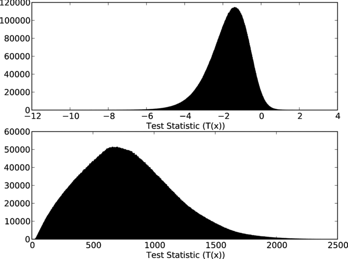
The test statistic is compared to a threshold to determine our level of confidence that the signal is real. To determine the threshold, we simulate 106 signal-present and 106 signal-absent sources, with the non-phase center signals distributed randomly in the field, and for S/Ns that reflect our data set. In addition, given that we expect the primary signals in the data to be RFI, rather than true signals, we also simulate zero-mean Gaussian noise with random RFI spikes located at a single time point in the visibilities. Figure 5 plots the log-scale distribution of the test statistics for both the signal-present (upper plot) and the signal-absent case (lower plot). The thresholds were chosen so as to minimize the chance of false positives, i.e., Type I error (Kay 1998, chap. 3). From Figure 5 the thresholds range from the maximum log of the test statistic for the signal-absent case (=2) to the minimum log of the test statistic for the signal-present case (=35).

Figure 5. Log-scale distribution of test statistics, ln [T(x)] obtained from Monte Carlo simulations for both (1) signal-absent (upper plot) and (2) signal-present (lower plot). Note the very different ranges plotted on the x-axis.
Download figure:
Standard image High-resolution imageThe method was then applied to the 200 narrowband signals, where the overall test statistic, T(x), was taken as the product of the test statistics of the individual baselines. Ten narrowband signals were found to have ln [T(x)] > 2 of which only two are beyond ln [T(x)] = 35 (Table 2). The data are expected to be consistent with no signal present at the phase center (i.e., consistent with the null hypothesis). The significance level of rejecting the null hypothesis (the p-value) for the 200 signals was found by integrating the probability distribution of the signal-absent test statistic, obtained from the simulations. A small p-value (p ⩽ 0.01) corresponds to a signal that may not be consistent with the null hypothesis and warrants further investigation. Figure 6 shows the p-values of the 200 signals. Most of the 200 signals were found to have a p-value greater than 0.01, with ten signals having a p-value of <0.01.

Figure 6. Distribution of p-values for the 200 narrowband signals. The p-values represent the error in rejecting the null hypothesis,  (signal-absent). The line plots the p = 0.01 significance value. Signals at or below this line can be considered inconsistent with the signal-absent hypothesis and require further analysis. The signals at p = 1 all have test statistics lower than the minimum test statistic of the simulated signal-absent distribution (Figure 5) and are assigned a p-value of 1.
Download figure:
Standard image High-resolution image
Table 2. The Ten Signals with ln [T(x)] > 2
| Frequency | UT | ln [T(x)] | Baseline Specific log of the Test Statistic | ||
|---|---|---|---|---|---|
| (MHz) | At–Mp | At–Pa | Pa–Mp | ||
| 1531.69080115 | 13:10:00–13:50:00 | 2.39 | 1.92 | −0.30 | 0.77 |
| 1533.6297203 | 09:10:00–09:50:00 | 3.11 | 6.12 | −1.36 | −1.65 |
| 1533.80206867 | 13:10:00–13:50:00 | 3.50 | 2.19 | 0.66 | 0.66 |
| 1527.85017443 | 09:10:00–09:50:00 | 4.21 | 4.89 | 1.40 | −2.07 |
| 1527.50351919 | 11:10:00–11:50:00 | 6.51 | 16.91 | −4.95 | −5.45 |
| 1527.56227431 | 11:10:00–11:50:00 | 7.25 | 11.04 | −0.27 | −3.52 |
| 1525.18856723 | 09:10:00–09:50:00 | 14.84 | 30.53 | −15.32 | −0.37 |
| 1527.50156068 | 09:10:00–09:50:00 | 26.19 | 17.86 | 2.87 | 5.47 |
| 1532.03158088 | 09:10:00-09:50:00 | 86.19 | 88.270 | 0.03 | −2.10 |
| 1527.56423282 | 09:10:00–09:50:00 | 242.77 | 1782.83 | −1305.76 | −234.30 |
Notes. Column 1: the center frequency; Column 2: the observed (UT) time period; Column 3: the sum of the log of the test statistics of the individual baselines, which is taken as the final test statistic; Columns 4–6: the log of the test statistics of the individual baselines.
Download table as: ASCIITypeset image
Eight signals lie between both distributions (2 < ln [T(x)] < 35). These signals are strictly inconsistent with both hypotheses and reflect the limitations of our simple analysis, namely, the simulation of data with either pure signals at the phase center or a single RFI peak in the visibility, and the need for the overall test statistic to have a value in excess of the threshold rather than those for the individual baselines.
Table 2 lists ln [T(x)] along with the test statistic for the individual baselines for all 10 events with ln [T(x)] > 2. For all but one of the 10 events, ln [T(x)] < 2 if the shortest baseline is excluded. For all 10 events the test statistic is far greater for the shorter baseline than for the other baselines. This is not consistent with a source at the phase center. It is, however, consistent with RFI distant from the phase center. We can therefore easily exclude these signals as being from the GL581 system.
5. DISCUSSION
We present the first VLBI SETI experiment. This pilot study demonstrates that the fundamental properties of VLBI make it an ideal technique for targeted SETI. With multiple baselines, milliarcsecond resolution, and millijansky sensitivities, RFI can be easily identified and rejected using automated techniques, while being sensitive to very weak signals.
Our search method targeted signals that are five times the baseline sensitivity, which were then cross-referenced over three baselines, to identify corresponding signals. Hence, the amplitude sensitivity of our array was limited to our least sensitive baseline over an 8 × 3 minute observing interval, for narrowband signals (At-Mp; 1σ = 0.31 mJy) and a single 3 minute scan for broadband signals (a factor of  less sensitive).9
Our experiment finds no evidence for radio signals >1.55 mJy (= 5σ) within the frequency range of 1230–1544 MHz from the region of Gl581. We can therefore place an upper limit of  on the power output of any isotropic emitter located in this planetary system, within this frequency range. On the other hand, the power of the Arecibo planetary radar transmitter is ∼1 MW (Black 2002; Tarter 2004). Assuming an aperture efficiency of 50%, at λ = 21 cm the directive power output is ∼6 TW. Over a bandwidth of 5.4 Hz (Black et al. 2001), this emission would have the flux density of a ∼200 Jy radio source (or 650 mJy if integrated over our channel width of 1.93 kHz) at a distance of 20 ly.
5.1. Using Current VLBI Instruments for SETI
Since this was a proof-of-concept observation, two differences between this experiment and a typical VLBI observation should be noted. First, the baseline lengths in this experiment were short by VLBI standards. Baselines one or even two orders of magnitude longer would significantly reduce the amount of correlated RFI. Second, most VLBI observations are carried out using more than three telescopes. Increasing the number of baselines to four or more constrains both the phase and amplitude closure relations,10 drastically increasing the quality of calibration. This would also provide the opportunity for image plane searching. However, it would likely be computationally expensive as a technique for searching over very wide frequency ranges. Relaxing the single baseline five times median limit could enhance the sensitivity beyond that of the weakest baseline.
We should also note that the width of the DFT bin is not a fundamental limit on the determination of the phase variation. A least-squares fit would allow the delay and delay rate to be determined more accurately. Essentially, the error on these parameters is limited by the signal to noise. Certainly, the LBA has been used for astrometry at the submilliarcsecond level (Deller et al. 2009b, 2009a). Observations of spacecraft have proven VLBI astrometry techniques for very weak narrowband sources (Avruch et al. 2006) and suggest that VLBI might even allow the detection of the orbital motion of SETI signals.
While the techniques discussed in this paper are ideal for targeted SETI, we also note the possibility of carrying out SETI commensally with normal VLBI operations. SETI target stars (Turnbull & Tarter 2003) would be expected to be present in the field of view of the antennas for VLBI observations reasonably regularly. Using the techniques discussed in Deller et al. (2011) and Morgan et al. (2011) it would be possible to produce visibility data sets for any target star in the primary beam. Additionally, direct analysis of the voltages (the baseband data) although computationally expensive could also be implemented at the correlator in an efficient manner to search for signals from extra-terrestrial intelligence. A possible model for this is the VFASTR transient search currently running at the VLBA operations center (Wayth et al. 2011; Thompson et al. 2011).
5.2. SETI and the Square Kilometre Array (SKA)
A sensitive and advanced radio telescope, the SKA is currently being planned for the coming decades.11
At 1400 MHz, the long baselines of the SKA will provide an astrometric precision of ∼10 μas (Fomalont & Reid 2004). In addition, the SKA is expected to achieve sub-μJy sensitivities (Carilli & Rawlings 2004). At ∼20 ly the SKA would probe an isotropic luminosity of a few  , far below the power output of radars and telecommunication satellites (Tarter 2004). The fields of view will be ∼1 deg2 at the maximum baselines and ∼30 deg2 for the shorter baselines (Carilli & Rawlings 2004). These capabilities will make the SKA the fastest, most sensitive, and widest field of view survey instrument in astronomy. However, for the SKA to be used for SETI, suitable targets are required. Such targets are currently being provided by the Kepler mission (Borucki et al. 2011; Batalha et al. 2012).
6. CONCLUSION
The discoveries of potential habitable planets are no doubt fueling a renewed excitement in SETI. With current VLBI systems we are able to search these candidates for signals from extra-terrestrial civilizations over a wide range of frequencies, and with high sensitivity.
In addition, VLBI is undergoing a transition from traditional recording systems toward real-time correlation via network connections (so-called e-VLBI). This has led to VLBI being used for rapid follow-up of transient sources. These developments, the wide range of frequencies covered by VLBI instruments, and the huge added value that VLBI techniques bring to a targeted SETI search make VLBI the natural choice for follow-up observations to confirm a potential SETI signal. However, more accurate positions are needed for target stars for future experiments with higher angular resolution. Such positions will be provided in the near future by the high-quality optical astrometry of Gaia (Bastian & Schilbach 1996).
The International Centre for Radio Astronomy Research is a joint venture between Curtin University and the University of Western Australia, funded by the state government of Western Australia and the joint venture partners. The Long Baseline Array is part of the Australia Telescope which is funded by the Commonwealth of Australia for operation as a National Facility managed by CSIRO. S.J.T. is a Western Australian Premier's Research Fellow, funded by the state government of Western Australia. The Centre for All-sky Astrophysics is an Australian Research Council Centre of Excellence, funded by grant CE11E0090. We thank Adam T. Deller for performing the correlation of the LBA data set, and James Miller-Jones for assisting in the calculation of the positional offset of Gliese 581.
Facilities: ATCA - Australia Telescope Compact Array, Mopra - Mopra Radio Telescope, Parkes - Parkes Radio Telescope
Footnotes
- 2
This is the projected angular distance as seen from Earth.
- 3
The reader is refereed to Bracewell (2000) for further details on discrete Fourier transforms.
- 4
- 5
The Astronomical Image Processing System (AIPS) was developed and is maintained by the National Radio Astronomy Observatory, which is operated by Associated Universities, Inc., under cooperative agreement with the National Science Foundation.
- 6
- 7
1 spectral channel = 1.95 kHz.
- 8
The International Mobile Satellite Organisation (INMARSAT) is an international treaty organization with 67 member countries including Australia. INMARSAT operates a GSO satellite system for global, mobile communications on land, sea, and in the air.
- 9
The sensitivity limits were derived using the System Equivalent Flux Densities (SEFD) for the individual telescopes at 1400 MHz; At = 68 Jy, Pa = 40 Jy, and Mp = 340 Jy.
- 10
The sum of the phases on any triangle of the three baselines and the combined amplitude ratio of four baselines contain information only on the true visibility of the source itself, all other errors cancel out (Thompson et al. 2001, chap. 9).
- 11