


Abstract
Monolayer structures made up of purely one kind of atom are fascinating. Many kinds of honeycomb systems including carbon, silicon, germanium, tin, phosphorus and arsenic have been shown to be stable. However, so far the structures are restricted to group-IV and V elements. In this work we systematically investigate the stability of monolayer structures made up of aluminium, in four different geometric configurations (planar, buckled, puckered and triangular), by employing density functional theory‐based electronic structure calculation. Our results on cohesive energy and phonon dispersion predict that only the planar honeycomb structure made up of aluminium is stable. We call it 'aluminene' according to the standard naming convention. It is a metal. Results of electronic band structure suggest that it may be regarded as a highly hole-doped graphene. We also present the tight-binding model and the Dirac theory to discuss the electronic properties of aluminene.
Export citation and abstract BibTeX RIS

Content from this work may be used under the terms of the Creative Commons Attribution 3.0 licence. Any further distribution of this work must maintain attribution to the author(s) and the title of the work, journal citation and DOI.
1. Introduction
Monolayer structures made up of purely one kind of atom possess many novel properties different from their bulk counterparts. The best example is graphene, which is a honeycomb monolayer of carbon [1, 2]. The other group-IV elements such as silicon, germanium and tin also form a honeycomb monolayer known as silicene, germanene and stanene, respectively [3–6]. Their geometric structures are buckled, where we can control the band gap by applying a transverse electric field [7–10]. They are expected to be topological insulators [4, 5]. Very recently, silicene has been experimentally demonstrated to act as a field-effect transistor at room temperature [11]. Phosphorene, honeycomb monolayer of phosphorus atoms, has experimentally been synthesized by exfoliating black phosphorus [12–14]. Its geometric structure is puckered. It is a direct-band gap semiconductor and possesses high hole mobility [15]. One can also tune the band gap by increasing the number of layers [15–17]. Another group-V honeycomb monolayer system (buckled and puckered structures) made up of arsenic atoms, called arsenene, has recently been predicted to be stable [18].
It is worth noting that so far there is no report available on monolayer structures composed of purely group-III elements. Though there exists a study on a boron-based finite triangular structure with a hexagonal hole, it lacks translational symmetry to form a periodic system [19]. Thus, it is important to probe whether group-III atom-based monolayer systems are stable and then investigate the physical properties of the stable ones.
With this motivation, we investigate the stability of monolayer structures made up of group-III elements (B, Al, Ga and In) and then study the geometric, electronic and vibrational properties by employing density functional theory (DFT) [20] based calculations. We consider four different geometrical configurations, namely, (a) planar, (b) buckled, (c) puckered and (d) triangular geometries. Our DFT-based phonon and cohesive energy calculations predict that among the above-mentioned four configurations of group-III elements, only the planar honeycomb monolayer made up of aluminium, as that of graphene, is stable. We call it 'aluminene' analogous to graphene. Further, we construct an 8-band tight-binding model and the Dirac theory to discuss the electronic properties of aluminene.
2. Computational details
We use the QUANTUM ESPRESSO package [21] to perform fully self-consistent DFT calculations [20] by solving the standard Kohn–Sham equations. For exchange-correlation (XC) potential, the generalized gradient approximation given by Perdew–Burke–Ernzerhof [22] has been utilized. We use Rappe–Rabe–Kaxiras–Joannopoulos ultrasoft pseudopotential [23] for Al atom which include the scalar-relativistic effect [24]. Kinetic energy cutoff of 50 Ry has been used for electronic wave functions. We adopt Monkhorst–Pack scheme for k-point sampling of the Brillouin zone integrations with 61 × 61 × 1, 51 × 51 × 1 and 51 × 41 × 1 for the triangular / buckled, planar and puckered systems, respectively. The convergence criteria for energy in SCF cycles is chosen to be 10−10 Ry. The geometric structures are fully optimized by minimizing the forces on individual atoms with the criterion that the total force on each atom is below 10−3 Ry/Bohr. In order to mimic the two-dimensional system, we employ a super cell geometry with a vacuum of about 18 Å in the direction perpendicular to the plane of monolayers so that the interaction between two adjacent unit cells in the periodic arrangement is negligible. To calculate the phonon spectra, we employ the density functional perturbation theory (DFPT) [25] implemented in PHonon code of the QUANTUM ESPRESSO package. The dynamical matrix is estimated with a 7 × 7 × 1 mesh of Q-points in the Brillouin zone.
3. Results and discussions
3.1. Stability
In order to study the stability of aluminene, we have carried out phonon dispersion calculations for all the geometric configurations. The fully optimized geometric structures and their corresponding phonon dispersion spectra are given in figure 1. Our calculations predict that planar aluminene with space group  forms a stable structure since it contains only positive frequencies for all the vibrational modes (figure 1(a)). On the other hand, the remaining geometric configurations possess structural instabilities in the transverse acoustic modes due to the presence of imaginary frequencies (shown as negative values). Cohesive energy for planar aluminene is estimated to be −1.956 eV and the negative value indicates that this is a bound system. Our calculations yield 4.486 and 2.590 Å for lattice constant and Al-Al bond length for the planar structure, respectively. After the geometry optimization the buckled (puckered) structure has become the AB (AA) bilayer of the triangular lattice (figures 1(b) and (c)). The relative displacement between the A and B layers is along the (1/3, 2/3, 0) direction. Since aluminene in triangular, buckled and puckered configurations is not stable, as observed from their phonon spectra, we do not consider them for further analysis.

Figure 1. Optimized geometries (top and side views) and phonon dispersion of aluminene in (a) planar, (b) buckled, (c) puckered and (d) triangular configurations. Planar aluminene is globally stable since the global minimum exists at the Γ point. There are negative phonons (corresponding to transverse acoustic modes) except for the planar configuration, indicating their instability. The blue lines in optimized geometry (top view) represent the unit cell.
Download figure:
Standard image High-resolution imageWe have also carried out phonon dispersion calculations for the planar, buckled, puckered and triangular configurations made up of other group-III elements (boron, gallium and indium). Our results show that there are no stable configurations.
3.2. Electronic structure
We present the results of the electronic band structure, density of states (DOS) and partial DOS (PDOS) for planar aluminene in figure 2(a). Aluminene behaves as a metallic system due to the partial occupancies in the σ as well as π bands. We wish to note that the other honeycomb monolayer materials studied so far are either semimetal or semiconductor. At the high symmetric K point in the Brillouin zone, two Dirac cones occur at energies 1.618 eV and  eV. The former is due to the π bonds purely made up of the pz orbital and the latter is due to σ bonds which has strong contribution from the s orbital. At the Fermi energy, there exist two σ bands and we call them the
  and
and  bands as shown in figure 3(a). The
  band is purely made up of px and py orbitals, while the mixing of the s orbital is not negligible in the
  band.
band.
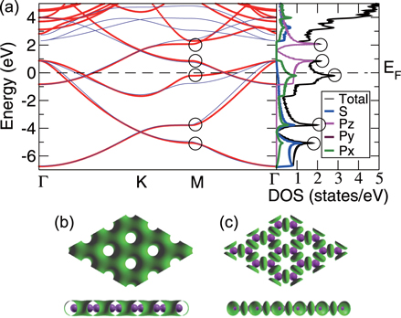
Figure 2. Planar aluminene. (a) Left panel: electronic band structure; right panel: total and partial DOS. Red curves are obtained from the first-principles calculation. Thin blue curves are obtained from the tight-binding model. Circles represent van Hove singularities, where the DOS is divergent. (b) Valence charge density. (c) Difference between the charge density of system and their atomic charge densities (top and side views).
Download figure:
Standard image High-resolution image
Figure 3. Planar aluminene. (a) Electronic bands which cross the Fermi level and (b) their Fermi surfaces (curves in 2D). One Fermi surface is hexagonally warped, while the other two Fermi surfaces are of circular shape.
Download figure:
Standard image High-resolution imageThe electronic band structure of aluminene closely resembles that of graphene [26], but the locations of the Dirac points in these two systems are different. In the case of graphene, the Dirac point lies exactly at the Fermi level where the bands due to the bonding orbitals (σ and π) are completely filled and those of anti-bonding orbitals are completely empty ( and
and  ). On the other hand, in aluminene, the bands due to the bonding orbitals (σ and π) are not completely filled and thus the Dirac point lies about 1.618 eV above the Fermi level. This is due to the fact that the number of valence electrons in Al (trivalent) is smaller than that of C (tetravalent). As a result, aluminene can be regarded as a highly hole-doped graphene. However, the important difference is that the Fermi energy is highly shifted in aluminene. Here, we wish to point out a remarkable feature of aluminene with respect to van Hove singularities. The van Hove singularity of the σ band exists very close to the Fermi energy at
  eV. It may be possible to tune the Fermi energy around the vanHove singularity and to make the electrical conductivity very large by applying gate voltage.
To understand the nature of bonding in aluminene, we have calculated the valence charge density (figure 2(b)). Except the hollow regions of hexagon, the charge is nearly uniformly extended over the aluminene plane which contributes to the conductivity. We have also calculated the difference between the charge densities of system and its atomic constituents (figure 2(c)). It clearly indicates the presence of covalent bonds between Al atoms in aluminene.
The transport properties of a metallic system are governed by the Fermi surface. The calculated Fermi surface for aluminene is given in figure 3(b). It consists of three closed loops, corresponding to the π,  and
and  bands. The momentum vectors at which the bands cross the Fermi level along high symmetric k-points are shown in figure 3(a). Magnitudes of momentum vectors along the Γ-K and Γ-M directions for the
  and π bands are equal (
 and
and  ). Furthermore, Fermi surfaces for these two bands are circular in shape around the Γ point. Thus, the electrons in these bands behave as free-particles. However, the magnitudes of momentum vectors along the Γ-K and Γ-M directions for the
  band are not equal (
 ). The Fermi surface for this band is highly hexagonally warped. We comment on these Fermi surfaces further when we analyze the Dirac theory as given below.
3.3. Tight-binding model
The electronic configuration of aluminium is [Ne] 3s23p1. We construct an 8-band tight-binding model including the 4 orbitals: 3s, 3px, 3py and 3pz. The tight-binding Hamiltonian is given by

where  denotes the nearest-neighbor transfer integral between the α orbital at the site i and the β orbital at the site j, and
  (
( ) annihilates (creates) an electron in the α orbital at the i site. We have derived the six independent Slater–Koster parameters (
 ,
,  ,
,  ,
,  ,
,  and
and  ) by fitting the DFT-based band structure at the Γ and K points, and present them in table 1. The tight-binding model reproduces the band structure near the Fermi energy well, as shown in figure 2(a). More details about the tight-binding model are given in appendix.
Table 1. The Slater–Koster parameters are obtained by fitting the DFT-based electronic band structure at the Γ and K points.
| Structure |

|

|

|

|

|

|
|---|---|---|---|---|---|---|
| Aluminene | 1.618 | −1.969 | −0.815 | −1.313 | −1.596 | −1.737 |
| Graphene [27] | 0 | −8.370 | −3.070 | −6.050 | −5.729 | −5.618 |
3.4. Dirac theory
We proceed to construct the Dirac theory to describe the band structure near the Fermi energy. First, the Fermi surface of the  band is highly anisotropic (see figure 3(b)). Hexagonal warping occurs due to the hexagonal symmetry at the Γ point. It is well described by the hexagonal warped Dirac Hamiltonian, which was originally proposed to describe the Dirac fermion on the surface of the 3D topological insulator [28],

where  is the velocity of Dirac fermion,
  describes the hexagonal warping effects,
  is the energy shift of the Dirac point,
  and
and  denotes the Pauli matrix. The energy is given by

It explains well the hexagonal warped Fermi surface shown in figure 3(b), where the values of the Fermi momenta  along the K direction and
  along the M direction are different (
 ).
).
We note that the low-energy Dirac theory is different from that of the minimal model of graphene made of the π bond, where the contribution from the σ bonds is negligible at the Fermi level. On the other hand, in aluminene, the σ bonds play a significant role to determine the electronic properties around the Fermi level. This difference arises because the Fermi energy in aluminene is much lower as compared to that in graphene. Namely, the Dirac Hamiltonian equation (2) is the continuum model of the σ bands at the Γ point. Hence, the theory of aluminene is different from the theory of graphene which is governed by the π band at the K point.
Next, the  band yields a circular shaped Fermi surface with
  . The
. The  band is described by the Hamiltonian equation (2) with
  and
and  .
.
Third, the π band also possesses a circular shaped Fermi surface with  . Around the Γ point, the Hamiltonian can be reduced to

We get the following energy for the above Hamiltonian,

leading to a circularly shaped Fermi surface with the radius

It is in good agreement with  obtained from the first-principles calculations.
4. Conclusion
We have demonstrated the stability of graphene-like honeycomb structure made up of aluminium, planar aluminene, from DFT-based phonon and cohesive energy calculations. It is a metal with partially filled σ and π bands. Our band structure calculations indicate that aluminene can be considered as a highly hole‐doped graphene. Fermi surface of this system contains features which correspond to free-electron-like and hexagonal warped surfaces. We obtain Slater–Koster parameters from the tight-binding model and construct the Dirac theory to explain the hexagonal warped Fermi surface of aluminene. Furthermore, we point out a remarkable feature of aluminene with respect to van Hove singularities. They emerge near the Fermi energy. They exist at  in the π band and at
  eV in the σ band. It is intriguing to note that chiral superconductivity is predicted to occur at the van Hove singularity of the π band in graphene [29]. We might expect a similar phenomenon to occur in aluminene. However, a study of this feature is beyond the scope of the present work.
Acknowledgments
C K and A C thank Dr G S Lodha and Dr P D Gupta for support and encouragement. They also thank the Scientific Computing Group, RRCAT for their support. M E is very much grateful to Prof N Nagaosa for many helpful discussions on the subject. He is also grateful for support by the Grants-in-Aid for MEXT KAKENHI grant number 25400317.
Appendix. Tight-binding model
We construct the tight-binding model which reproduces the band structure obtained from the first-principles calculation. The electronic configuration of aluminium is [Ne] 3s23p1. It is enough to include the 4 orbitals:  , 3px, 3py and 3pz. In the planar honeycomb system, the pz orbital has no overlap with the other orbitals since its wave function is antisymmetric with respect to the honeycomb plane, while the wave functions of the other orbitals are symmetric. Hence, the Hamiltonian is block diagonalized into two sub-matrices: one is the 2-band model which gives one π-bond, while the other is the 6-band model which gives three σ bonds. The model is identical to the 8-band tight-binding model of graphene including the σ bonds [26].
The tight-binding Hamiltonian is given by

where  denotes the nearest-neighbor transfer integral between the α orbital at the site i and the β orbital at the site j. The Hamiltonian has 6 independent Slater–Koster parameters:
  ,
,  ,
,  ,
,  ,
,  and
and  . We fix these parameters by fitting the band structure obtained from the first-principles calculation at the Γ and K points. The fitted parameters are shown in table 1 of the main text. The Dirac cone exists at
  for the π bands.
A.1. π bonds
The Hamiltonian for the π bonds is given by

with

which is the same as the tight-binding model of graphene with only the pz orbitals being included.
By explicitly diagonalizing the Hamiltonian, we obtain the energies  at the K point and
  the Γ point as

By solving the energies at the K and the Γ, we get

By comparing the energies of π at these high symmetric points, which are obtained from the DFT (shown in table A1
njp516911t2), we find the two Slater–Koster parameters ( and
and  ) and the values of these two parameters are given in table 1 of the main text.
Table A1. The energy obtained by the first-principles calculations at the Γ and K points.
| Structure |

|

|

|

|

|

|
|---|---|---|---|---|---|---|
| Aluminene | 1.618 | −0.828 | −4.274 | −6.757 | 0.871 | 2.819 |
A.2. σ bonds
For the σ bond, we take the following basis,  . The Hamiltonian for the σ bonds has the form

with

and

where the matrix elements are given by
We can determine the energy at the Γ point as

and at the K point as

By solving the energies at the K and the Γ, we obtain

Again, we find the above-mentioned four Slater–Koster parameters by comparing the energies obtained from the DFT calculations (shown in table A1), and the results are summarized in table 1 of the main text.
A.3.
 bands
bands

It is enough to take into account only the px and py orbitals to describe the  bands. The Hamiltonian for this case is given by

and

with the matrix elements given in equation (A.9). We call it the px–py model.