
Abstract
The concern about Arctic greening has grown recently as the phenomenon is thought to have significant influence on global climate via atmospheric carbon emissions. Earlier work on Arctic vegetation highlighted the role of summer sea ice decline in the enhanced warming and greening phenomena observed in the region, but did not contain enough details for spatially characterizing the interactions between sea ice, temperature and vegetation photosynthetic absorption. By using 1 km resolution data from the Moderate Resolution Imaging Spectrometer (MODIS) as a primary data source, this study presents detailed maps of vegetation and temperature trends for the Siberian Arctic region, using the time integrated normalized difference vegetation index (TI-NDVI) and summer warmth index (SWI) calculated for the period 2000–11 to represent vegetation greenness and temperature respectively. Spatio-temporal relationships between the two indices and summer sea ice conditions were investigated with transects at eight locations using sea ice concentration data from the Special Sensor Microwave/Imager (SSM/I). In addition, the derived vegetation and temperature trends were compared among major Arctic vegetation types and bioclimate subzones. The fine resolution trend map produced confirms the overall greening (+1% yr−1) and warming (+0.27% yr−1) of the region, reported in previous studies, but also reveals browning areas. The causes of such local decreases in vegetation, while surrounding areas are experiencing the opposite reaction to changing conditions, are still unclear. Overall correlations between sea ice concentration and SWI as well as TI-NDVI decreased in strength with increasing distance from the coast, with a particularly pronounced pattern in the case of SWI. SWI appears to be driving TI-NDVI in many cases, but not systematically, highlighting the presence of limiting factors other than temperature for plant growth in the region. Further unravelling those limiting factors constitutes a priority in future research. This study demonstrates the use of medium resolution remotely sensed data for studying the complexity of spatio-temporal vegetation dynamics in the Arctic.
Export citation and abstract BibTeX RIS

Content from this work may be used under the terms of the Creative Commons Attribution-NonCommercial-ShareAlike 3.0 licence. Any further distribution of this work must maintain attribution to the author(s) and the title of the work, journal citation and DOI.
1. Introduction
Recent warming trends have been greater over the Arctic than on average on the planet (Chapman and Walsh 1993, Serreze and Francis 2006, Winton 2006, Kaufman et al 2009, Hansen et al 2010). These studies report on average warming 3–4 times higher for the Arctic than globally over the past decade. Similarly, vegetation changes have recently been observed over the Arctic. Myneni et al (1997), Zhou et al (2001) and Hudson and Henry (2009) found that Arctic vegetation biomass tends to increase, resulting in a higher photosynthetic absorption. Many authors have demonstrated the link between the warming and the changes in vegetation recently observed (Jia et al 2003, Walker et al 2006, Olthof and Latifovic 2007, Epstein et al 2008, Raynolds et al 2008, Hill and Henry 2011, Elmendorf et al 2012). Specifically, these changes concern an increase in plant height as well as plant biomass and modifications in plant communities composition, such as increasing shrub proportion (Chapin et al 1995, Sturm et al 2001b, Tape et al 2006, Walker et al 2006, Hudson and Henry 2009) and are associated with an increase in photosynthetic absorption, expressed as the normalized difference vegetation index (NDVI) (Jia et al 2009, Walker et al 2009, Beck and Goetz 2011). Such changes in Arctic vegetation characteristics may result in significant effects on both local and global climates due to complex feedback mechanisms (Chapin et al 2000, Dutta et al 2006, Schuur et al 2008, Von Deimling et al 2011).
The surface energy balance approach is often used to describe those processes relating vegetation cover to permafrost thaw. Eugster et al (2000) state that due to an increase in the proportion of shrubs regional temperature will rise as a consequence of the lower canopy albedo of shrubs as compared to tundra. However, an increase in air temperature does not necessarily relate to an increase in soil temperature. Blok et al (2010) showed that due to the shading effect of their canopy, an increase in shrub cover (Betula nana) would lead to a different partitioning of net radiations, resulting in a reduction of the ground heat flux. Summer permafrost thaw would be reduced in that case. However, Betula nana expansion could as well have the opposite impact during winter, given their snow trapping capacity providing insulation for the soils to winter temperatures (Sturm et al 2001a). For the purpose of climate predictions, it is therefore essential to further understand the evolution of vegetation in the Arctic under temperature changes.
In addition to changes in vegetation, Arctic sea ice conditions are also rapidly changing. Comiso et al (2008) and Comiso and Nishio (2008) observed an Arctic-wide summer sea ice retreat, particularly pronounced during the past decade. This retreat is thought to have a large impact on local temperature and climate via the low albedo of open water as compared to sea ice (Bhatt et al 2010, Serreze and Barry 2011). This warmer climate in turn would enhance vegetation productivity and thus greening.
Many studies have used the satellite measured NDVI as the greenness indicator for the Arctic. The index relates to photosynthetic absorption of the vegetation and provides a fair approximation of the biomass production when integrated over time (Reed et al 1994). Both time integrated NDVI (TI-NDVI) and maximum NDVI (MaxNDVI) have been widely used in Arctic vegetation studies (Stow et al 2004). TI-NDVI reflects biomass production while MaxNDVI provides information about the seasonal peak of photosynthetic absorption. Values of TI-NDVI and MaxNDVI over the Arctic range from 20 to 85 and from 0.03 to 0.70 respectively (Walker et al 2005, Bhatt et al 2010). These indices can be assembled over several years to create time series from which trends can be derived and investigated. Various space borne sensors have systematically acquired spectral data of the earth surface, including the Arctic regions, providing time series covering up to 29 years in the case of the AVHRR sensors. The products delivered to the end users contain processed NDVI data at various spatial resolutions. A commonly used dataset in NDVI trend analysis is the Global Inventory Modeling and Mapping Studies (GIMMS) dataset (Tucker et al 2005). Derived from data acquired from AVHRR sensors, this dataset is composed of a continuous time series starting in 1981 at a spatial resolution of 8 km. GIMMS data are synchronized to cope with inconsistency issues due to sensor successions. In 2000 the first of the Moderate Resolution Imaging Spectroradiometer (MODIS) sensors was launched. Although providing shorter time series, MODIS sensors have a finer spatial resolution and are usually considered to be more accurate due to a narrower band sampling and the fact that, unlike AVHRR sensors, MODIS was specifically designed for vegetation monitoring (Huete et al 2002). They can therefore complement the long time series analysis performed at lower spatial resolution using AVHRR derived datasets.
Using GIMMS long time series, Bhatt et al (2010) have shown that proximity to the sea impacts vegetation dynamics in the Arctic regions. The main hypothesis for explaining this mechanism lies in the impact that summer sea ice has on near shore land temperature, and hence on vegetation. Although Bhatt et al (2010) noticed differences regarding the effect of sea ice on TI-NDVI between near shore areas and the full tundra domain, the relation between sea distance and Arctic vegetation productivity has not yet been established. Furthermore, the level of details of the results obtained does not allow for a spatial characterization of the influence of sea ice decline, such as variation in strength of the correlation with increasing distance to the sea, to be achieved. A better characterization of the impacts of sea ice decline on both temperature and vegetation is required for predictions to be made about the evolution of the Arctic in future climate scenarios. Adding a spatial component to those existing studies will be of great value for vegetation modelling and eventually permafrost and carbon emission modelling.
In this study, we mapped vegetation and temperature trends for the Siberian Arctic, based on 1 km resolution MODIS time series spanning the 2000–11 period. In this way we not only reveal the potential of MODIS time series for detecting trends, but we also provide the finest resolution trend maps of the region to date. Furthermore, by relating the SWI and TI-NDVI time series with near shore sea ice concentration time series for several locations, we determine the spatio-temporal relationship between sea ice conditions, temperature and vegetation photosynthetic absorption. In order to further understand the spatial variability of the observed greening, we compared average TI-NDVI trends among the main vegetation classes and bioclimate subzones.
2. Material and methods
2.1. Study area
Figure 1 presents the study area with the different sub-regions considered. For consistency and comparability, these sub-regions were defined based on boundaries used by Bhatt et al (2010), with each region named after the sea it is facing. The map also displays locations of the transects used in the analysis to investigate the effect of distance from the coast on the relationship between sea ice and TI-NDVI and SWI, as well as the areas considered for integrating sea ice concentration time series in the analysis. Arctic boundaries are based on the map produced by the CAVM, for which the Arctic extent was defined as the strip bounded by the sea at the north and the start of the boreal forest at the south (Walker et al 2002, 2005). Eight locations, defining the start of the transects, were distributed along the coast. Those selected locations and transects are a way to study the local phenomenon of enhanced local warming and greening related to sea ice decline, including a spatial component. In order to study a potential directional effect of sea ice concentration on the land parameters, we set three transects going inland for each location. The middle transect is oriented directly towards the south while the south east and south west transects are oriented at 150° and 210° respectively. Each transect is 50 km wide, has a maximum length of 300 km and is divided in distance classes of 25 km. Areas of potential sea ice influence are defined by a round 150 km buffer in the seaward direction from the start of the transect (figure 1).
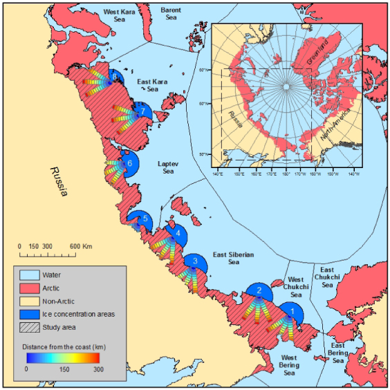
Figure 1. Map presenting the study area, the sub-regions considered, and the local transects. Arctic extent is based on CAVM datasets. The eight local regions are later referred to in the article as 1: West Chukchi, 2: East Siberia East, 3: East Siberia Centre, 4: East Siberia West, 5: Laptev East, 6: Laptev West, 7: East Kara East, 8: East Kara West.
Download figure:
Standard image2.2. Data and products derived
All data of land surface variables used in this study are derived from data acquired by the MODIS Terra sensor. MODIS Terra data have been acquired on a daily basis since 2000 with the launch of the first MODIS sensor. Raw data and composite products are available at different resolutions from the United States Geological Survey Distributed Active Archive Center (USGS-DAAC)1. Processed NDVI is available in the form of 16 days data composites and land surface temperature (LST) in the form of 8 days data composites. Both products were downloaded at 1 km spatial resolution. Data composites combine in one tile the pixels with the highest value (NDVI), or with an average of all cloud free observations values (LST) over the considered period. In this way, clouded pixels are filtered out in most cases, and cloud free composites can be delivered. For this study, data from the Terra sensor alone were used, since they provide a longer time series than the MODIS Aqua sensor. The MODIS Land Cover Type product, available at the same spatial resolution, was used in order to identify and filter out water bodies.
Sea ice concentration data were obtained from the Special Sensor Microwave Imager (SSM/I) data, downloaded from the National Snow and Ice Data Center (NSIDC) website2. The elaboration of the product, based on passive microwave brightness temperatures data, is described in Comiso and Nishio (2008) and Maslanik and Stroeve (1999). These data are acquired daily at a 25 km spatial resolution for the whole Arctic basin. The pre-processed time series, currently only available up to the year 2010, was extended for the year 2011 using the near-real-time sea ice extend product.
Different shapefiles produced by the CAVM team were used in the study, including the arctic boundary map for defining the extent of the study area and the vegetation map and bioclimatic region map (Walker et al 2005) for further explaining spatial patterns in vegetation trends. The vegetation classes that constitute the vegetation map were derived from data of the 1993–5 period (Walker et al 2005). Despite the fact that changes are occurring in the region and the accuracy of vegetation classes boundaries is up for discussion (Lloyd 2005, Goetz et al 2011, Epstein et al 2012), the data are considered suitable for the large scale vegetation trend study presented here. All data used for this study are listed in table 1.
Table 1. List of data products used.
| Product name | Product type | Resolution | Period considered |
|---|---|---|---|
| MOD13A2 | NDVI | 1 km | 2000–11 |
| MOD11A2 | LST | 1 km | 2000–11 |
| MOD12Q1 | Land cover type | 1 km | 2004 |
| (—) | Circumpolar arctic coastline and tree line boundary | (Vector map) | (—) |
| (—) | Circumpolar arctic vegetation map | (Vector map) | (—) |
| (—) | Circumpolar arctic bioclimate subzones | (Vector map) | (—) |
| NSIDC-0002 | DMSP, SSM/I-SSMIS daily polar gridded bootstrap sea ice concentrations | 25 km | 2000–10 |
| NSIDC-0081 | Near-real-time DMSP SSM/I-SSMIS daily polar gridded sea ice concentrations | 25 km | 2011 |
2.3. Pre-processing
Pre-processing of the time series was required prior to the calculation of the indices used later in the analysis. Although composite products were used (8 and 16 days for LST and NDVI respectively), some clouded pixels were detected and masked, creating temporal gaps in the time series. Such pixels were re-calculated using a temporal filter, interpolating or replacing values based on the quality control values of the two surrounding dates. In the rare situations when three or more consecutive clouded pixels were detected in the time series, the entire time series was not further used in the analysis. This mainly occurred for some rare pixels in the Bering/Chukchi region, where extended periods of cloud cover are apparently frequent. In addition, day 177 of the year 2001, that was missing due to sensor malfunctioning, had to be created, also using temporal linear interpolation. TI-NDVI was calculated as the sum of NDVI values above 0.05 for each composite between May and September. Similarly SWI, expressed in growing degree days (GDD), corresponds to the sum of temperature above freezing along a year. In this way, SWI relates to the warmth beneficial to plant growth during the summer period. This warmth metric has been used in the past in several Arctic vegetation studies, either derived from satellite (Raynolds et al 2008, Walker et al 2009, Bhatt et al 2010) or ground (Jia et al 2003, 2006, Walker et al 2012) temperature measurements, and has been shown to relate well with greenness, particularly in these warmth-limited environments. For this study, SWI was computed at a 1 km resolution for each year by summing the 8 day composites of LST above 0 °C for the same period as used in TI-NDVI calculation. For normalization of the units, values obtained by adding the composites over the season were multiplied by 8 and 16 for SWI and TI-NDVI respectively, based on the length of the composites in days.
Although the relationship has not yet been established for this indicator specifically in the tundra biome, we assumed that using TI-NDVI as the greenness indicator would provide a fair estimate of above ground biomass. Recently, Walker et al (2012) and Raynolds et al (2012) demonstrated the existence of a strong correlation between MaxNDVI, defined as the peak NDVI value throughout the vegetation season, and aboveground phytomass for the tundra biome. We believe that an integrated index such as the TI-NDVI should also provide a fair indication of biomass, as it captures both the aspects of maximum value over the vegetation season and the total accumulated photosynthetic activity, beneficial to the biomass accumulation in the non-chlorophyll part of the plant (Tucker and Sellers 1986).
2.4. Analysis
Sea ice concentration time series were constructed from SSM/I data for each location defined by the sea buffer presented in figure 1. Assembling such data in time series analysis requires the definition of a fixed date for considering concentration among years. This timing was defined independently for each location by taking the period at which the inter-annual average sea ice concentration is 50%. This choice of considering 50% sea ice concentration for the definition of sea ice timing is based on analysis made by Bhatt et al (2010) concerning a strong correlation between sea ice concentration around this period and near shore land temperature. The time series was constructed for each location by averaging the daily sea ice concentration data for a 10 day period centred around this fixed date. Correlations between sea ice concentration, SWI and TI-NDVI were calculated on linearly detrended time series. Detrending consists of removing the best fit linear function to the time series and results in removing the effect of the trend while keeping the annual variability. Correlations between detrended time series therefore indicate the correlation between annual variations of the two variables. Significance levels were assessed using a two tailed t test for correlations and based on the Mann Kendall test for trend values. The Mann Kendall test was preferred to the t test as it provides significance values based on ranking and is therefore more suitable when working with time series (De Beurs and Henebry 2005). However, it is important to note that p-values obtained from this test are independent from the strength of the trend, but rather influenced by the consistency of the change.
3. Results and discussion
3.1. Overall trends
Figure 2 presents the trend values of TI-NDVI and SWI on a pixel basis for the entire study area. Overall, the region is greening and warming, but local browning and cooling spots can also be observed. The main cooling patterns are located between the east Kara and Laptev regions and in west Bering, while browning areas are of lower extent and are mainly located in the east Siberian region and in the east of the Laptev region. The yearly change in SWI ranges between −1.1% and 1.5% (defined as the 5 and 95 percentiles of the entire range) with an average of 0.22%, while TI-NDVI yearly change rates range between −0.4% and 3% and average 1.17%. Negative trends are therefore more pronounced and more frequent in the case of SWI than for TI-NDVI. The latter metric, on the other hand, displays greater positive trends, meaning that greening is often more pronounced than warming.

Figure 2. Trend maps of the study area for SWI (left) and TI-NDVI (right) time series. Both indices are derived from MODIS terra sensor observation period 2000–11. Sectors used to derive sea ice concentration trends are depicted on both maps in order to facilitate a joint reading with table 2.
Download figure:
Standard imageWhen taken in consideration with the results presented in table 2, the trends shown in figure 2 are consistent with the theory that sea ice influences temperature and vegetation trends. According to this hypothesis, land regions facing sea areas with the greatest ice decline should experience the greatest warming and greening. East Kara East and West are experiencing important sea ice decline, of −4.9% and −3.6% respectively. Land areas facing these two sea locations also present trend values that are among the greatest of the entire study area. On the other hand, East Siberia Centre, which depicts a slightly positive increase in sea ice concentration over the period 2000–2011 faces a land area only experiencing slight warming and greening and partly browning and cooling. It appears then that land areas facing the sea regions with large decreases in sea ice concentration are experiencing the greatest greening and warming trends, while on the other hand greening and warming are more moderate near areas of low change in sea ice concentration. Low significance levels for ice trends in those regions where ice retreat is confirmed can be attributed to large annual variations in ice concentration, hence strongly influencing the output of the rank based Mann Kendall test. Those trends therefore ought to be considered significant.
Table 2. Trend values of sea concentration between 2000 and 2011 for the eight locations of the study area. The sea ice timing corresponds to the period from which the concentration time series were derived. Note that trends are not significant (p = 0.05).
| Location | Average yearly sea ice change (%) | Sea ice timing |
|---|---|---|
| 1: West Chukchi | 0.3 | 1/06–10/06 |
| 2: East Siberia East | −2.2 | 21/06–30/06 |
| 3: East Siberia Centre | 1.1 | 21/06–30/06 |
| 4: East Siberia West | −0.6 | 11/06–20/06 |
| 5: Laptev East | −0.8 | 1/06–10/06 |
| 6: Laptev West | −2.4 | 11/06–20/06 |
| 7: East Kara East | −4.9 | 11/06–20/06 |
| 8: East Kara West | −3.6 | 1/06–10/06 |
Figure 3 presents SWI and TI-NDVI time series for the five Arctic sub-regions, Bering, Chukchi, Siberian, Laptev and Kara, with the trend values and significance levels associated. All regions present a positive trend for both TI-NDVI and SWI but the variability is large among regions as well as between SWI and TI-NDVI. Largest yearly change values are found for Chukchi (0.61%) and Laptev (1.4%) for SWI and TI-NDVI respectively, with Laptev showing the only significant trend for p = 0.05. The trend values reported here can be compared with values reported by Bhatt et al (2010) for the same regions based on the GIMMS3g dataset. However, in order to be compared, values provided in Bhatt et al (2010) have to be divided by the length of the time series they used, that is to say 26 years. Among the five regions of Siberian Arctic, Bhatt et al (2010) also found Chukchi and Laptev to have the largest trends for SWI and TI-NDVI respectively. However, results reported using the GIMMS3g 26-year time series show great differences with this study. Regarding TI-NDVI, two regions, Bering and Chukchi, were reported in Bhatt et al (2010) as having negative trends with annual changes of −0.077% and −0.15% respectively, while all trends calculated over the last 12 years here are positive. The consistently higher TI-NDVI trend values over the 12 years of MODIS than for the 26 years AVHRR time series may indicate an acceleration of the greening process of the Arctic through the last decade. Even though the GIMMS dataset and consequently its arctic version, the GIMMS3g dataset, were created considering several issues such as sensor successions or satellites drift (Pinzon et al 2004, Tucker et al 2005), the data came from AVHRR sensors, which were not originally designed for vegetation monitoring, and for that reason are usually considered less accurate than MODIS sensors (Huete et al 2002). Fensholt and Proud (2012) carried out a comparative study between the two NDVI datasets and found large differences particularly for high latitude areas, indicating potential inconsistencies and shortcomings of GIMMS3g. It is therefore likely that the higher TI-NDVI trends found in this study, compared to Bhatt et al (2010) are a combination of datasets inconsistencies and accelerated greening. Regarding SWI, trend values reported by Bhatt et al (2010) are surprisingly much higher than values reported in this study. The maximum relative difference is found for the Bering region, with a trend value 30 times lower using the MODIS time series than with AVHRR temperature data. The absolute difference in SWI annual change for the Bering region between the two studies is 1.6%.

Figure 3. Regional time series of SWI (red) and TI-NDVI (green) for the five regions of interest of the study area. Dotted lines represent the linear trend of the time series while coloured number indicate the yearly percentage change. Significance of the trend at the 95% or greater, based on the Mann Kendall test are marked with an asterisk (*).
Download figure:
Standard imageIt is therefore clear that time series trend analysis using MODIS is a valuable contribution to longer GIMMS3g based analysis. Although shorter in time, data are more reliable for reasons such as sensor narrower band widths (Huete et al 2002), consistency in the technology and the higher spatial resolution. Increased spatial resolution, from 8 km to 1 km in this case, allows for greater potential to discriminate among land classes, hence reducing the mixed pixel effect. The enhanced trend maps presented in figure 2 confirm the overall greening detected in previous studies, but also reveal higher greening trend values for the period 2000–11 than for the 1982–2008 period. Those differences are likely to be partly the result of an accelerated greening. On the other hand, a potential accelerated warming remains to be confirmed, since differences observed in SWI trends between the two datasets would suggest a decrease of the warming intensity over the last decade. Such results contradict most climate scenario studies (Serreze and Barry 2011). For that reason, we believe that inconsistencies between the two datasets are at the origin of these differences. Further investigation, involving comparison of results over matching periods and detailed comparison of the processing chains, is required to track the origin of these differences in temperature trends.
3.2. Spatial characterization of TI-NDVI and SWI trends
In an attempt to further characterize spatial variations in TI-NDVI trends, we calculated zonal statistics for the land cover and bioclimate subzones classes of the CAVM dataset (Walker et al 2005). Both maps can be viewed and downloaded on the CAVM project website3. The results of this analysis are presented in figure 4. For each vegetation class and bioclimate subzone, the surface area of the box is proportional to relative area occupied by the class in the study area.

Figure 4. Boxplots comparing the effect of land cover (a) and bioclimate subzone (b) on TI-NDVI trends. The surfaces of the boxes are proportional to the relative area occupied by the class in the study area, and bottom and top of the boxes are the lower and upper quartiles, respectively. TI-NDVI trends are expressed in annual percentage change.
Download figure:
Standard imageEach land cover type is likely to evolve differently, and a change in land cover is likely to affect the response of the TI-NDVI signal to increasing biomass in a nonlinear manner. Figure 4, which shows the boxplots of TI-NDVI trend per CAVM vegetation class, does not show clear evidence that specific plant functional types are displaying stronger relative increases in productivity than others. What can be noted is that the Barren classes and the classes G1, P1, G2 and W1 do have the highest average increases in TI-NDVI. This can be caused by their location, since these vegetation classes are mostly located in the northern parts of the Arctic. On the one hand this can support the idea that the decrease in sea ice extent leads to a stronger increase in TI-NDVI near the coast. On the other hand, these vegetation classes are characterized by a low net annual productivity. Therefore, small absolute increases in productivity will be shown as large relative increases. This can also be observed when looking at the boxplot of TI-NDVI trend per bioclimate subzones. These are defined by the yearly sum of temperature they receive, and spatially distributed from north to south. As a consequence of this geographical positioning, they receive decreasing influence from the sea. In the case of the study area, subzones B and C are essentially coastal zones, while D and E are shared between coastal and inland areas. Subzone A is hardly present in our study area and is consequently represented by a highly variable narrow box. Overall, in figure 4(b) the positive TI-NDVI trend decreases southward. The difference can be particularly noticed between subzones B and C and subzones D and E. When going from A to E, the subzones are characterized by a strong increase in net annual productivity (Walker et al 2005). The observed relative change is strongest further north, but it should be noted that these are also the areas that do have a low annual net productivity.
3.3. TI-NDVI, SWI and sea ice concentration interdependences
Figure 5, presents the correlation value between SWI and TI-NDVI detrended time series. The correlation between the two variables is generally positive, meaning that annual variations in one variable vary in the same way as annual variation in the other variable. Only a few locations present negative correlations, and those cases are of low intensity and not statistically significant. As a result, those pixels represent locations where detrended time series are independent, rather than negatively correlated. One hypothesis for the absence of correlation is that temperature, or the number of growing degree days per year, is not limiting the growth of vegetation, but rather another variable acts as a limiting factor. Walker et al (2009) presented a schematic of factors potentially able to affect plant growth in Arctic regions (figure 10 in their article), as well as potential interactions and feedbacks existing between these factors. It appears from their schematic that multiple site factors, including soil, landform, hydrology, permafrost and microclimate, are expected to have an influence on plant growth. Although, the present study provides little information on the respective importance of these factors, it can certainly orientate further research aiming at unravelling limiting factors for plant growth in the Arctic. Despite the relatively short time series—hence limiting the number of observations—a large proportion of pixels present significance levels above p = 0.05. We believe that longer time series would set the significance thresholds lower, while maintaining correlation values observed. The relatively low proportion of significant pixels is therefore highly related to the length of the time series used.
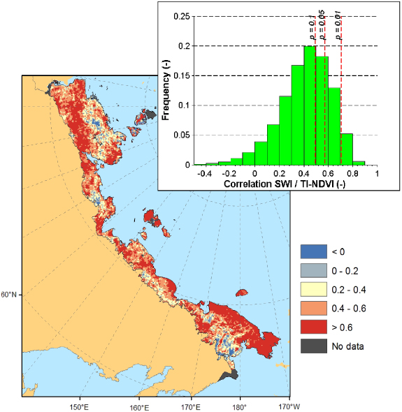
Figure 5. Map depicting the spatial distribution of the correlation between SWI and TI-NDVI detrended time series for the study area. The histogram in the corner presents the frequency of coefficients, with p-values associated.
Download figure:
Standard imageIn order to further characterize the effect of proximity with the sea, sea ice concentration, which is the assumed driving factor of the greening and warming amplification effect, was included in the analysis. For each location, we correlated detrended sea ice concentration time series with detrended SWI and TI-NDVI time series, for several distance classes. Full results for two specific locations are given in figure 6. The two profiles present particularly interesting cases. The profile of East Siberia East location shows a pattern as expected, with the strength of the correlation between detrended time series for both variables increasing as a function of decreasing distance to the sea, suggesting that a decrease in sea ice concentration leads to a higher SWI and a higher TI-NDVI. The difference in correlation strength between the two variables and sea ice concentration is also as expected for this profile, with SWI having a constantly stronger correlation with sea ice than TI-NDVI. Such difference is coherent with the theory of sea ice having a direct influence on SWI, but a more indirect influence on TI-NDVI, with SWI being the intermediate factor. On the other hand, the TI-NDVI profile of East Siberia West location shows a positive correlation with sea ice concentration near the coast, evolving to a negative correlation when moving away from the shore. The reasons for obtaining such an extreme profile remain an open question. The SWI profile at the same location depicts a constant negative correlation value independent from the distance to the coast. These transects, located in East Siberia West, spatially coincide with an area of weak correlation between SWI and TI-NDVI detrended time series, which explains the divergence between the two profiles. However, as stated earlier, we cannot be certain of the reasons behind this lack of relation for some locations between SWI and TI-NDVI. Overall, for the eight locations, the expected profile with negative correlation decreasing in strength as distance with the sea increases could be found 6 times for SWI, but only 4 times in the case of TI-NDVI, and in nearly all cases the correlation was constantly stronger for SWI than for TI-NDVI. This difference confirms the direct relationship between near shore sea ice concentration and SWI and the more indirect characteristic of the relationship with TI-NDVI. In all eight cases, the three profiles, corresponding to the three directions investigated did not diverge sufficiently to suggest a directional effect of sea ice concentration on SWI and TI-NDVI.
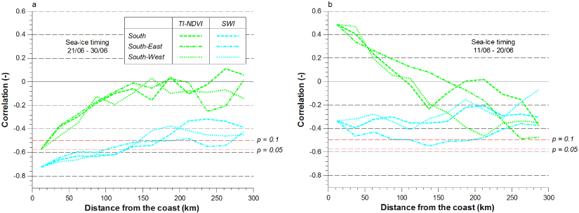
Figure 6. Spatial profiles of correlation between ice concentration and TI-NDVI and SWI detrended time series for the period 2000–11 for the two locations East Siberia East (a) and East Siberia West (b).
Download figure:
Standard imageA summary profile for both SWI and TI-NDVI based on the average correlations from the middle transect is presented in figure 7. In the case of TI-NDVI, the large variability of the correlation makes the information difficult to be summarized. The envelope is therefore particularly extended, showing the large spatial variability of the relationship and therefore an inconsistent response pattern to sea ice concentration variations. The pattern highlighted earlier is more visible in the case of SWI, with a strong negative correlation with sea ice near the shore and a decrease in the strength of this correlation as distance to the coast increases. Also, the extent of the envelop is more restricted than in the case of TI-NDVI, hence confirming a greater spatial consistency in the sea ice–SWI relationship than in the relationship between sea ice and TI-NDVI.
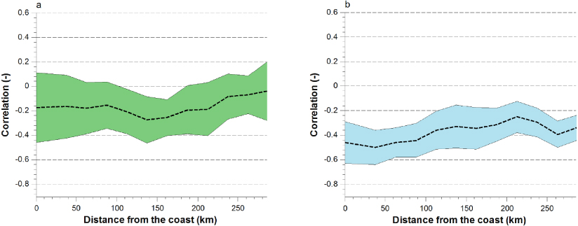
Figure 7. Average profile of correlation between detrended sea ice concentration time series and detrended TI-NDVI (a) and SWI (b) time series. The envelope around the average profile corresponds to ±2 standard errors. The right end of the profile does not include measurement for all locations since the transect length is limited in certain cases to the Arctic extent width, which may not reach 300 km.
Download figure:
Standard imageThose results concerning the relation between sea ice concentration and SWI strengthen theories on a well-documented phenomenon, stating that sea ice concentration has an influence on temperature (Serreze and Barry 2011). The values of correlation with sea ice detrended time series found here correspond well with values reported in Bhatt et al (2010), with averages of −0.40 and −0.41 for SWI and TI-NDVI respectively, for the entire Eurasia. While the sea ice concentration–SWI relation is relatively spatially consistent, the relation between sea ice concentration and TI-NDVI presents greater spatial variability. These areas of low correlation between sea ice concentration and TI-NDVI seem to be associated with areas also depicting weak SWI–TI-NDVI correlation. Therefore, linking greening of tundra ecosystems to sea ice decline requires TI-NDVI to be driven by SWI. One bottleneck in our understanding of the Arctic vegetation systems is this relationship between SWI and TI-NDVI. The hypothesis for explaining those areas where vegetation appears to behave independently from temperature concerns a limitation of plant growth potential by factors other than temperature (Walker et al 2012). Comparable results were found as part of a plot based study conducted on plots located in North America and Northern Europe, with plant communities presenting spatially non-uniform response to warming (Elmendorf et al 2012). The current state of knowledge is limited on this topic and therefore needs to be broadened. Future research should investigate more into details the limiting factors of vegetation growth, and the potential to integrate such in situ variables in large scale studies. Best outputs will certainly be achieved by combining detailed data collected at a plot level with consistent regional remote sensing time series. Our ability to predict the evolution of vegetation for this region greatly depends upon the understanding we have of interrelations between all variables recorded in the past years. Such predictions would have multiple benefits as it would for instance allow permafrost modelling studies to integrate an accurate vegetation component in their models (Blok et al 2010), later enabling more realistic carbon emission predictions for the Arctic regions (Riseborough et al 2008).
4. Conclusion
Vegetation dynamics and drivers of Arctic greening need to be better understood as they are of high relevance in global climate dynamics. The spatio-temporal relationships between temperature, greenness and sea ice concentration were investigated for the Siberian Arctic tundra, with SWI and TI-NDVI used as temperature and greenness indicators respectively. The use of MODIS as the data source is one major difference in the approach with previous work. Although spanning a shorter period than the GIMMS3g dataset, MODIS data provide more accurate data with a higher spatial resolution. As a result, the study revealed the potential of a 12 year time series derived from MODIS to detect trends in vegetation and temperature and produced a high spatial resolution trend map for the Siberian Arctic. Overall the region is greening and warming, but patches of browning and cooling could be observed as well. Although annual variations in SWI are shown to explain a large part of TI-NDVI annual variations, putting temperature rise as an essential driver of greening, the amount of pixels presenting total independence between the two variables was found to be non-negligible as well. This absence of relation reveals the existence of factors other than temperature limiting vegetation growth in the Siberian Arctic. By adding time series of sea ice concentration in the analysis, it was possible to investigate how annual variations in sea ice conditions spatially correlate with both SWI and TI-NDVI. While the pattern of sea ice concentration influence on SWI is quite constant along the coast, with the strength of the relationship decreasing with increasing distance to the shore, the reaction of TI-NDVI presents a greater spatial variability. Areas of low correlation between sea ice concentration and TI-NDVI correspond to areas where vegetation growth is not temperature driven. This correspondence strengthens the theory that SWI plays an essential intermediate role in the influence of sea ice on vegetation productivity, but also emphasizes the need for further research to unravel the drivers, other than temperature, of vegetation growth in the Siberian Arctic. By better characterizing spatio-temporal relationships between sea ice, temperature and vegetation, this study contributes to the understanding of some key Arctic vegetation dynamics, essential in the current climate and carbon debate.